Galaxy Clustering and Large–Scale Structure
from $z=0.2$ to $z=0.5$ in Two Norris Redshift Surveys

Abstract

We present a study of the nature and evolution of large–scale structure based on two independent redshift surveys of faint field galaxies conducted with the 176–fiber Norris Spectrograph on the Palomar 200–inch telescope. The two surveys sparsely cover $\sim 20$ sq. degrees and contain 835 $r\leq 21$ mag galaxies with redshifts $0.2<z<0.5$. Both surveys have a median redshift of $z_{\rm med}\approx 0.30$. In order to obtain a rough estimate of the cosmic variance, we analyze the two surveys independently.

We have measured the two–point spatial correlation function and the pairwise velocity dispersion for galaxies with $0.2<z<0.5$. We measure the comoving correlation length to be $3.70\pm 0.13h^{-1}$ Mpc ($q_{0}=0.5$) at $z_{\rm med}=0.30$ with a power–law slope $\gamma=1.77\pm 0.05$. Dividing the sample into low ($0.2<z<0.3$) and high ($0.3<z<0.5$) redshift intervals, we find no evidence for a change in the comoving correlation length over the redshift range $0.2<z<0.5$. Similar to the well–established results in the local universe, we find that intrinsically bright galaxies are more strongly clustered than intrinsically faint galaxies and that galaxies with little ongoing star formation, as judged from the rest–frame equivalent width of the [O II]$\lambda$3727, are more strongly clustered than galaxies with significant ongoing star formation. The rest–frame pairwise velocity dispersion of the sample is $326^{+67}_{-52}$ km s^-1, $\sim 25$% lower than typical values measured locally. Our sample is still too small to obtain useful constraints on mean flows.

The appearance of the galaxy distribution, particularly in the more densely sampled Abell 104 field, is quite striking. The pattern of sheets and voids which has been observed locally continues at least to $z\lesssim 0.5$. A friends–of–friends analysis of the galaxy distribution supports the visual impression that $\gtrsim 90$% of all galaxies at $z\lesssim 0.5$ are part of larger structures with overdensities of $\gtrsim 5$, although these numbers are sensitive to the precise parameters chosen for the friends–of–friends algorithm.

1 Introduction

The clustering of galaxies is customarily characterized by a hierarchy of n–point correlation functions (Peebles 1980), although, in practice, only the two–point correlation function, $\xi(r)$, can be measured accurately with current redshift surveys. For local, optically–selected samples, $\xi(r)$ is well–described by a power law, $\xi(r)=(r/r_{0})^{-\gamma}$, with correlation length $r_{0}\approx 5h^{-1}$ Mpc ($h$ is the present value of the Hubble constant measured in units of 100 km s^-1 Mpc^-1) and slope $\gamma\approx 1.8$ for $r\lesssim 20h^{-1}$ Mpc (Loveday et al. 1995; Marzke et al. 1995; Guzzo et al. 1997; Jing, Mo, & Börner 1998). At higher redshifts, the strength of the clustering can be inferred from the two–point angular correlation function or measured directly from a redshift survey. Angular correlation function studies are essential for understanding the clustering of faint objects beyond the spectroscopic reach of current facilities and for reducing cosmic variance by covering large areas (Brainerd & Smail 1998, Postman et al. 1998). However, such studies must rely on models of the redshift distribution of faint galaxies to deduce the three–dimensional correlation length.

With the recent completion of large redshift surveys of galaxies with redshifts up to $z\sim 1$ (e.g., Lilly et al. 1995a [CFRS]; Ellis et al. 1996 [Autofib]; Cowie et al. 1996 [Hawaii]; Yee, Ellingson, & Carlberg 1996 [CNOCI]; Small, Sargent, & Hamilton 1997a [Norris]; Carlberg et al. 1999 [CNOCII]), it is now possible to measure the evolution of clustering directly. Having been principally designed to study the redshift–evolution of the galaxy population (to which they have made landmark contributions), the CFRS, Autofib, and Hawaii surveys are not particularly well–suited to studying large–scale structure, mainly because they do not extend over large contiguous areas of the sky. Using the Autofib survey, Cole et al. (1994) measured $\xi(r)$ for $z\lesssim 0.3$ and found no evidence for evolution in the comoving correlation length. In contrast, Le Fèvre et al. (1996) observed rapid decline of the correlation length with redshift for galaxies observed in the Canada–France Redshift Survey. Shepherd et al. (1997) used data from the CNOCI cluster survey to measure a correlation length at $z\sim 1/3$ consistent with the evolution inferred by Le Fèvre et al. (1996). The correlation length of galaxies from the Hawaii K–band–selected sample exhibits a similar decline over a large redshift range from $z\sim 0.3$ to $z\sim 1.4$ (Carlberg et al. 1997).

The differing results for the redshift–evolution of galaxy clustering reached so far emphasize the need for larger surveys to map large–scale structure and to limit the impact of field–to–field variance. Indeed, Postman et al. (1998) from their I–band imaging survey of 16 sq. deg. infer a correlation length at $z=0.5$ twice as large as that found, for example, in the CFRS. Our two Norris surveys of the fields of the Corona Borealis supercluster and the Abell 104 galaxy cluster, while not as deep as the CFRS, Autofib, Hawaii, and CNOC surveys, cover (albeit sparsely) fields of 16 sq. degrees and 4 sq. degrees, respectively, and include a total comoving volume between $0.2<z<0.5$ of $2\times 10^{6}h^{-3}$ Mpc³ ($q_{0}=0.5$). Both Norris surveys, with the foreground supercluster and cluster regions removed, have median redshifts of 0.3, and each contains several hundred $r\leq 21$ mag galaxies with redshifts in the interval $0.2<z<0.5$. We expect any overall density fluctuation,

$${\delta\bar{n}\over\bar{n}}\sim{J_{3}\overwithdelims( )V}^{1/2}$$ (1)

(Davis & Huchra 1982), where $J_{3}$ is the second moment of the two–point spatial correlation function (Peebles 1980) and is approximately equal to $10,000h^{-1}$ Mpc³ (Tucker et al. 1997), in our survey volume $V$ to be $\lesssim 10$%. This is comparable to the statistical error in our estimates of the correlation strength at $1h^{-1}$ Mpc. The only survey with comparable power for exploring large–scale structure at intermediate–redshifts is the recently–completed CNOCII survey (Carlberg et al. 1999). The CNOCII survey contains five times as many galaxies as our two surveys combined but covers only 10% of the area (in four separate survey zones). The preliminary results of the CNOCII survey presented by Carlberg et al. (1999) are in general agreement with and complementary to the main conclusions presented in this paper.

Observations of galaxy clustering such as those described here cannot, however, be interpreted in a straightforward fashion because one may not be observing the same types of galaxies at high redshift as at low redshift. In local samples, early-type galaxies are clustered more strongly than late-type galaxies (Loveday et al. 1995, Guzzo et al. 1997). The importance of accounting for the change in the observed galaxy population is illustrated by the strong clustering exhibited by the Lyman–break galaxies at $z\sim 3$ (Steidel et al. 1997, Giavalisco et al. 1998). This strong clustering, with a correlation length at least twice as large as that observed at $z\sim 1$ by Le Fèvre et al. (1996), can be naturally explained if the Lyman–break galaxies are highly biased with respect to the mass distribution (Bagla 1998, Steidel et al. 1998). The likely variation of bias with redshift and among different galaxy populations at the same redshift will complicate efforts to test the gravitational instability hypothesis and to determine the mass density of the universe, but it also implies that studies of the growth of clustering can help us to understand bias and galaxy formation.

The observed two–point correlation function, which is expected to be isotropic in real space when averaged over a sufficiently large volume, is distorted in redshift space by line–of–sight peculiar velocities. (For a comprehensive review, see Hamilton 1998.) On small scales, the velocity dispersion of bound clusters of galaxies suppresses the apparent correlation function, whereas coherent motions of galaxies towards overdense regions and away from underdense regions enhance the correlation function on large scales. An analysis of the distortions allows one in principle to measure the moments of the distribution of pairwise velocity distribution. As is well known, both the first and second moments can be used to estimate the mean density of the universe, $\Omega_{0}$ (modulo the bias parameter). However, we will not attempt to do so here since survey volumes substantially larger than ours are required to obtain interesting results (Fisher et al. 1994).

Our data are, nevertheless, well–suited to a measurement of the pairwise velocity dispersion of galaxies, $\sigma_{12}$. The pairwise velocity dispersion is a measure of the kinetic energy in the galaxy distribution. Since $\sigma_{12}$ is a pair–weighted statistic and thus very sensitive to the number and treatment of rich clusters in the survey volume, it is difficult to compare values of $\sigma_{12}$ measured in different redshift surveys and with $\sigma_{12}$ determined in large $N$–body simulations in a consistent fashion. The first measurement of the pairwise velocity dispersion, $\sigma_{12}=340\pm 40$ km s^-1, was obtained by Davis & Peebles (1983) using data from the CfA1 redshift survey. Subsequent measurements, including a reanalysis of the CfA1 data by Somerville, Davis, & Primack (1997), have demonstrated as much as a factor of 2 variation in $\sigma_{12}$ depending on the type and environment of galaxies analyzed and on the treatment of rich clusters (e.g., Mo, Jing, & Börner 1993; Zurek et al. 1994, Marzke et al. 1995; Guzzo et al. 1997; Jing, Mo, & Börner 1998). However, redshift surveys are becoming large enough and analysis techniques sophisticated enough to begin to measure reliable values of $\sigma_{12}$. The large volume of our combined surveys, $\sim 2\times 10^{6}h^{-3}$ Mpc³ (comoving, $q_{0}=0.5$), will enable us to make a measurement of $\sigma_{12}$ at intermediate redshift for which the error due to cosmic variance will be $\lesssim 20$% (Marzke et al. 1995), similar in size, in fact, to our statistical error.

We describe our data in the following section, §2. The techniques we use to compute the correlation function are outlined in §3, and we present the results of this analysis in §4. We discuss the pairwise velocity dispersion $\sigma_{12}$ at $z_{\rm med}=0.30$ in §5. In §6, we consider the large–scale structure of the galaxy distribution in our sample and quantify the clustering on 10 to 100 $h^{-1}$ Mpc scales with a friends–of–friends analysis. Finally, we summarize our results and discuss the redshift evolution of $\xi$ and $\sigma_{12}$ in §7. We use $q_{0}=0.5$ in the main discussion and for the figures except where explicitly noted.

2 Data

Our analysis is based on data we have obtained with the 176–fiber Norris Spectrograph (Hamilton et al. 1993) on the Palomar 5 m telescope. We have surveyed two fields, one centered on the $z\approx 0.07$ Corona Borealis supercluster (R.A. = $15^{h}30^{m}$, Dec. = $+30^{\circ}$) and the other on the $z\approx 0.08$ Abell 104 galaxy cluster (R.A. = $0^{h}45^{m}$, Dec. = $+24^{\circ}$). The Norris Spectrograph is designed for redshift surveys of faint galaxies. Its fibers are only 2 m long in order to minimize light losses due to absorption in the fibers, and the fiber entrance aperture is only 1.6 arcsec (FWHM), which maximizes the contrast of a $r\sim 20-21$ mag object against the Palomar sky. Norris is equipped with a sensitive, thinned, backside–illuminated, anti–reflection–coated SITe 2048² CCD. Due to the large plate scale (2.55 arcsec/mm) of the Cassegrain focus of the 5 m telescope, the fibers can be placed within 16 arcsec of each other, allowing comoving scales as small as $0.1h^{-1}$ Mpc to be probed at $z\sim 0.3$. Smaller scales can be probed by observing a given field more than once. Our velocity accuracy, judged from repeat observations, is $\sim 75$ km s^-1.

For each galaxy, we estimate a coarse spectral type based on its Gunn $g-r$ color, where the magnitudes are measured from POSS-II $J$ and $F$ plates of the fields, and its redshift. We classify the galaxies into spectral classes based on the E, Sbc, Scd, and Im spectral energy distributions compiled by Coleman, Wu, & Weedman (1980). The spectral type is a real number that takes the values of 0 for an elliptical galaxy, 2 for an Sbc galaxy, 3 for an Scd galaxy, and 4 for an Im galaxy. We interpolate between the Coleman et al. (1980) spectral energy distributions to construct the spectral energy distribution appropriate for the give spectral type. Finally, we use the interpolated spectral energy distribution to compute the $k$–correction necessary to transform between apparent and absolute magnitude. (For a more extensive discussion of our spectral classification and computation of absolute magnitudes, see Small, Sargent, & Hamilton [1997b].)

The Norris data suffer from both magnitude and spatial selection effects. We assume that the total selection function is separable:

$$S(m,\alpha,\delta)=s_{m}(m)\times s_{\alpha,\delta}(\alpha,\delta),$$ (2)

where $s_{m}(m)$ is the probability that a galaxy with magnitude $m$ is sufficiently well detected to yield a secure redshift and $s_{\alpha,\delta}(\alpha,\delta)$, where $\alpha$ and $\delta$ are celestial coordinates, is the geometrical modulation of $s_{m}(m)$ (c.f. Yee et al. 1996). The mean value of $s_{\alpha,\delta}$ is approximately one. We could also account for the fraction of objects that are classified as galaxies in the original catalog from which we select objects but which turn out to be misclassified stars. However, since this fraction is small ($\sim 10$%) and does not vary spatially, we have chosen to ignore it. The precise forms of $s_{m}$ and $s_{\alpha,\delta}$ for the two surveys are described in the following two subsections.

2.1 The Corona Borealis Survey

The survey of the Corona Borealis supercluster has already been described in the literature (Small, Sargent, & Hamilton 1997a), and so we will only briefly review the salient points here. The core of the supercluster covers a $6\arcdeg\times 6\arcdeg$ region of the sky and consists of seven rich Abell clusters. Since the field of view of the Norris Spectrograph is 20′ in diameter, we planned to observe 36 fields selected from the POSS-II survey (Reid et al. 1991) and arranged in a rectangular grid with a grid spacing of 1°, with the precise position of a particular field adjusted to maximize the number of fibers placed on galaxies. We mainly tried to avoid the cores of the seven Abell clusters since redshifts for many galaxies in the cores are available from the literature. We successfully observed 23 of the program fields and 9 additional fields along the ridge of galaxies between Abell 2061 and Abell 2067, yielding redshifts for 1491 extragalactic objects. Our first 17 fields were observed when no large–format $2048^{2}$ CCD was available at Palomar, limiting us to using only one-half of the fibers and leading to geometrical selection effects for which we are not able to correct. We have therefore restricted the analysis presented here to the 981 $r<21$ mag, $z<0.5$ galaxies successfully observed with the large–format $2048^{2}$ CCD available at Palomar since 1994. Excluding the data from the first 17 fields observed only reduces the number of galaxies at $0.2<z<0.5$ by 23%. The locations on the plane of the sky of all the galaxies in the Corona Borealis survey are shown in Figure 1. Galaxies with $z>0.2$ are marked with filled circles while galaxies with $z\leq 0.2$ are marked with unfilled circles.

The redshift distribution for all galaxies with $r\leq 21$ mag is shown in Figure 2. The prominent features at $z\approx 0.07$ and $z\approx 0.11$ are the two superclusters in the field; see Small et al. (1998) for a detailed discussion of the properties of the superclusters. In our analysis of the field galaxy luminosity function in the Corona Borealis survey (Small et al. 1997b), we found that the region from $0<z\leq 0.2$, with the superclusters excluded, was overdense by 21% relative to other high–Galactic–latitude fields. While this overdensity is not an exceptional fluctuation, we have conservatively chosen to avoid the complications of analyzing such a large overdense region and have limited our study to galaxies with $0.2<z<0.5$. The galaxy number density over this redshift range is consistent with the number density found in the CFRS (Lilly et al. 1995b) and CNOCII (Lin et al. 1998) surveys.

The Corona Borealis survey is not magnitude–limited. In Figure 3, we plot $s_{m}(m)$, the ratio of the number of galaxies with measured redshifts to the total number of galaxies in the survey fields as a function of magnitude. For $16\lesssim r\lesssim 18.5$, the ratio $s_{m}(m)$ is nearly constant, but below unity because of sparse sampling. It then falls rather steeply to fainter magnitudes due both to the fiber assignment algorithm and to the increasing difficulty of measuring redshifts for fainter objects. Since the light from very bright galaxies can bleed into neighboring fibers, we have made a modest effort to avoid galaxies brighter than $r\lesssim 16$ mag, which accounts for the decline in the fraction of galaxies observed at the brightest magnitudes. We describe how we correct for magnitude incompleteness in §3.

Our sampling of the Corona Borealis field on the plane of the sky varies dramatically. In particular, much of the $6^{\circ}\times 6^{\circ}$ has not been surveyed at all. We quantify the angular selection effects by dividing the entire survey area into $103\times 103$ 9 sq. arcmin cells and, for each cell, computing the ratio of the number of galaxies with magnitudes $15\leq r\leq 21$ with measured redshifts to the total number of catalog galaxies with magnitudes $15\leq r\leq 21$. The 9 sq. arcmin cells are as small as we can make them while still maintaining a reasonable number of galaxies in each cell. The geometrical selection function, $s_{\alpha,\delta}$, is this ratio normalized by the fraction (16%) of $15<r<21$ magnitude galaxies in the survey fields for which we have obtained reliable redshifts. The mean value of $s_{\alpha,\delta}$ averaged over the survey fields is 0.99. We display the map of $s_{\alpha,\delta}$, Gaussian–smoothed with $\sigma=1$′ for clarity, in Figure 4. The gray scale ranges linearly from 0. to 2.0, and the contours are drawn at 0.5, 1.0, and 1.5. The most prominent feature of the map is the radial dependence of the sampling within a given Norris field. The decline in sensitivity at the edges of the field is due to a combination of effects: mild vignetting, curvature of the focal plane which makes fibers at the edge slightly out of focus, and a bias against pairs with large angular separation introduced by the fiber assignment software (see Small et al. 1997a).

Since the survey area has been divided into $3^{\prime}\times 3^{\prime}$ cells, this procedure does not correct for spatial selection effects on scales smaller than 3′. The fibers cannot be placed within 16″ of each other, and so we expect a substantial deficit of observed pairs on scales smaller than $\sim 50$ arcsec. This deficit is illustrated in Figure 5 in which we plot, as a function of pair separation, the ratio of the number of observed pairs of galaxies to the number of pairs, averaged over 50 realizations, of galaxies selected from the survey fields according to the total selection function (i.e., magnitude selection times geometrical selection). There is a strong bias against observed pairs with separations smaller than 100″. When computing correlation functions, we use the ratio shown in Figure 5 to correct the observed pair counts for these missing small–angular–separation pairs. (This correction is described in more detail in §3.) The plot in Figure 5 also reveals a significant deficit of pairs with angular separations ranging from 13′ to 33′, scales comparable 20′ field–of–view of the Norris spectrograph. Since there are so few observed pairs with separations on this scale, we cannot accurately correct for missing pairs on this scale and simply leave a gap in the correlation function at the physical scale corresponding to this angular scale ($\sim 5h^{-1}$ Mpc at $z\sim 0.3$). We do not attempt to measure correlations on scales larger than 30′ and therefore ignore the imperfections in our model of the geometrical selection effects on large scales.

2.2 Abell 104 Survey

The data from our Abell 104 survey are similar in most respects to the data obtained in our Corona Borealis survey. We have surveyed 1 sq. deg. centered on Abell 104, plus four outlying fields northeast, northwest, southeast, and southwest of the center by $\sim 1.5^{\circ}$. We have measured spectra for 1330 galaxies in the survey, 207 of which lie in Abell 104 at $z\approx 0.08$. We have 558 galaxies with redshifts $0.2<z<0.5$ and magnitudes $15<r<21$. The locations on the sky of these 558 galaxies (filled circles), along with the locations of the $r<21$ mag galaxies with $z<0.2$ (unfilled circles), are shown in Figure 6. The survey will be described in detail in Small, Sargent, & Hamilton (1999).

As with the Corona Borealis survey, the A104 survey is not magnitude–limited. A plot of $s_{m}(m)$, the ratio of the number of galaxies with measured redshifts to the total number of galaxies in the survey fields as a function of magnitude, is shown in Figure 7. The A104 field is less sparsely sampled than the Corona Borealis field. The magnitude selection function declines slowly from $r\approx 15$ mag to $r\approx 20$ mag, beyond which the selection function drops sharply. The A104 survey is modestly deeper than the Corona Borealis survey, principally because the experience gained during the Corona Borealis survey was successfully applied to the A104 survey. The increased depth of the A104 survey is borne out in the redshift distribution plotted in Figure 8.

The A104 survey, like the Corona Borealis survey, suffers from uneven spatial sampling. We construct a map of the spatial selection function $s_{\alpha,\delta}$ for galaxies with $15\leq r\leq 21$ in the same manner as for the Corona Borealis survey. We divide the entire survey region into $38\times 38$ square cells, each of which has an area of 9 sq. arcmin. For each cell, the angular selection function is the number of galaxies with measured redshifts with magnitude $15\leq r\leq 21$ divided by the total number of galaxies with magnitude $15\leq r\leq 21$, normalized by the fraction (22%) of galaxies in the entire survey for which we have obtained reliable redshifts. The mean value of $s_{\alpha,\delta}$ is 0.98. This map is shown in Figure 9. The gray scale ranges linearly from 0. to 2., and the contours are drawn at 0.5, 1.0, and 1.5. The spatial selection function is higher in the central field because the central field was observed multiple times. The multiple observations of the central field also increase the number of close pairs, although a significant bias against close pairs remains. In Figure 10, we plot, as a function of angular separation, the ratio of the number of pairs of galaxies successfully observed to the number of pairs, averaged over 50 realizations, of galaxies in the parent catalog selected according to the combined magnitude and spatial selection functions. Due to the overlapping Norris fields in the A104 survey, the sampling of pairs as a function of angular separation is noticeably more uniform than for the Corona Borealis survey. In particular, there is no deficit of pairs on scales comparable to the size of the Norris field–of–view. Of course, as for the Corona Borealis survey, the spatial selection function can only correct for errors on angular scales larger than the $3^{\prime}\times 3^{\prime}$ cell size in which the selection function was computed. Thus, there is still a large error on scales smaller than 180″, in the sense that close pairs are excluded from the redshift survey, which is shown in the inset in Figure 10. When computing correlation functions, we use an additional selection function to correct the smallest angular scales. This additional function is simply the ratio of pair separations for separations less than 200″, multiplied by 1.04 to bring the flat part of the function to a mean value of 1.

3 Definition and Computation of $\xi(r_{p},\pi)$ and $\xi(r)$

Redshift–space maps of the spatial distribution of galaxies are distorted by the peculiar motions of galaxies because the measured redshift of a galaxy is the sum of the Hubble motion of the galaxy plus the line–of–sight peculiar velocity. The most prominent signatures of redshift–space distortions are the “fingers of God” seen in redshift surveys of rich clusters of galaxies, in which the large velocity dispersion of a cluster spreads out the cluster galaxies along the line–of–sight in redshift space. On large scales, coherent infall into overdense regions and outflow from underdense regions enhance the correlation function. Since the velocities on large scales can be simply related to the mean mass density of the universe $\Omega_{0}$ with linear theory, an analysis of redshift space distortions can in principle yield an estimate of $\Omega_{0}$ (Sargent & Turner 1977, Fisher et al. 1994, Hamilton 1998). The distribution of galaxies on the plane of the sky is not, however, distorted by peculiar velocities. Thus, correlation functions, which one assumes are isotropic in real space when averaged over sufficiently large volumes, are anisotropic in redshift space. It is, therefore, useful to compute correlation functions as functions of separations along the line–of–sight ($r_{\pi}$) and perpendicular to the line–of–sight ($r_{p}$).

The two-point correlation function $\xi(r_{p},r_{\pi})$ is defined implicitly by the following equation for the joint probability $\delta P$ of finding a galaxy in each of two volume elements $dV_{1},dV_{2}$ separated by $r_{p}$ and $r_{\pi}$,

$$\delta P=\bar{n}^{2}[1+\xi(r_{p},r_{\pi})]dV_{1}dV_{2},$$ (3)

where $\bar{n}$ is the mean galaxy density. In order to compute $\xi(r_{p},r_{\pi})$, we construct a catalog of randomly distributed points with the same selection function as the real data. We estimate $\xi(r_{p},r_{\pi})$ using the estimator derived, tested, and recommended by Landy & Szalay (1993):

$$\xi(r_{p},r_{\pi})={DD(r_{p},r_{\pi})-2DR(r_{p},r_{\pi})+RR(r_{p},r_{\pi})\over{RR(r_{p},r_{\pi})}},$$ (4)

where DD$(r_{p},r_{\pi})$, RR$(r_{p},r_{\pi})$, and DR$(r_{p},r_{\pi})$ are the number of data–data, random–random, and data–random pairs, respectively, with separations $r_{p}$ and $r_{\pi}$. There are three important virtues of Landy & Szalay’s estimator: it is affected only in second order by density fluctuations on the scale of the survey; it does not require an independent measurement of the mean density of the survey; and its errors are very nearly Poissonian for an unclustered population.

The data–data pair counts are corrected for missing pairs on small scales using the curves shown in Figures 5 and 10. As expected and demonstrated below, the correction works very well for the angular correlation function. In applying this correction to the spatial correlation function, we simply assume, since the bias against close separation pairs is primarily due to limits on how closely fibers can be placed in the focal plane of the spectrograph, that the redshift distribution of unobserved close pairs is identical to that of observed close pairs.

In order to compute the real space correlation function $\xi(r)$, we follow Davis & Peebles (1983), and many subsequent workers, by projecting $\xi(r_{p},r_{\pi})$ onto the $r_{p}$ axis. The projection $w_{p}(r_{p})$ depends only on the real space correlation function:

$$w_{p}(r_{p})=2\int_{0}^{\infty}\xi(r_{p},r_{\pi})dr_{\pi}=2\int_{0}^{\infty}\xi[(r_{p}^{2}+y^{2})^{1/2}]dy,$$ (5)

where $y$ is the line–of–sight separation in real space. The integrand in the second expression for $w_{p}(r_{p})$ is the correlation function in real space. If we assume that $\xi(r)=(r/r_{0})^{-\gamma}$, where $r_{0}$ is the correlation length and $\gamma$ is the power–law index, the integral for $w_{p}(r_{p})$ can be evaluated analytically to give:

$$w_{p}(r_{p})=r_{p}{r_{0}\overwithdelims( )r_{p}}^{\gamma}{\Gamma{1\overwithdelims( )2}\Gamma{\gamma-1\overwithdelims( )2}\over{\Gamma{\gamma\overwithdelims( )2}}},$$ (6)

where $\Gamma$ is the standard gamma function. By fitting a power law to $w_{p}(r_{p})$, we can determine the correlation length $r_{0}$ and power law index $\gamma$ of the real space correlation function.

We calculate the error in $\xi(r_{p},r_{\pi})$ using the standard technique of bootstrap resampling the data (Ling, Frenk, & Barrow 1986). We perform 50 bootstrap resamples with replacement and take the error bars on $\xi(r_{p},r_{\pi})$ to be the standard deviation of the bootstrap estimates. The bootstrap error bars are typically 75–100% larger than error bars derived from the standard Poisson estimate, $\sigma(\xi)=(1+\xi)/\sqrt{DD}$.

The construction of the random catalog is complicated by our magnitude selection effects and our uneven spatial sampling. As noted above, our sample of galaxies is not magnitude-limited. In addition, it is important that the color distribution of the galaxies in the random catalog matches the observed color distribution. We have, therefore, selected the redshifts of galaxies in the random catalog not from the probability distribution $P(M|z)$ that an object at redshift $z$ has an absolute magnitude $M$, which would be appropriate for a magnitude–limited sample, but rather from the distribution $P(z|m,type)$ that a galaxy with an apparent magnitude $m$ and spectral type $type$ (rounded to E, Sbc, Scd, or Im; see §2) has a redshift $z$ (suggested by D. Hogg, personal communication):

$$P(z|m,type)={\phi[M(z,m,type)]{dV\over{dz}}\over{\int_{0}^{\infty}\phi[M(z^{\prime},m,type)]{dV\over{dz^{\prime}}}dz^{\prime}}}.$$ (7)

Here, $\phi(M)$ is the luminosity function, $M(z,m,type)$ is the absolute magnitude of a galaxy of spectral type $type$ such that it would have apparent magnitude $m$ at redshift $z$, and $dV/dz$ is the comoving relativistic volume element. For each galaxy in the survey, we generate 100 galaxies in the random catalog with the same apparent magnitude and spectral type as the given galaxy, with redshifts drawn according to Equation 7, and with celestial coordinates distributed according to the spatial sampling maps presented in §2. Thus, the distribution of apparent magnitudes and spectral types of the galaxies in the random catalog is identical to that of the real survey data, but the locations are random. Note that when analyzing a subset of the survey data selected by spectral type or intrinsic luminosity, it is trivial with this method to ensure that the random catalog is generated with exactly the same selection function.

We use a Schechter (1976) function to describe the luminosity function of our survey. For $0.2<z<0.5$, we use Schechter parameters $\alpha=-0.85$ and $M^{\ast}=-19.45+5\log h$ ($q_{0}=0.5$) in the $B_{AB}$–band, consistent with the results from the CNOCII survey (Lin et al. 1998) and our own survey (Small et al. 1997b). Luminosity functions constructed from the combined A104 and Corona Borealis surveys agree very well with a Schechter function with these parameters. The normalization of the luminosity function drops out of Equation 7.

Since our method for generating the redshifts of the galaxies in the random catalog is novel and our spatial selection effects are quite dramatic, we have conducted two tests to verify that our techniques are working correctly. First, to test our corrections for our spatial selection effects, we have compared the two–point angular correlation function, $\omega(\theta)$, of galaxies selected from the parent photometric catalog according to the magnitude selection function (referred to as the “photometric sample” below) with the angular correlation function of the galaxies with measured redshifts (c.f., Shepherd et al. 1997). We have estimated $\omega(\theta)$ using the Landy–Szalay estimator. In order to estimate the errors for the angular correlation function of the photometric sample, we have computed the angular correlation function for 50 samples selected from the photometric catalog and averaged the results. The angular correlation functions for the Corona Borealis and Abell 104 photometric and redshift samples are plotted in Figure 11. The correlation functions of the redshift samples, with bootstrap error bars, are plotted both with and without corrections for missing pairs on small scales ($<600$″ for the Corona Borealis survey and $<200$″ for the Abell 104 survey). Without this correction, the correlation functions fall significantly below the correlation functions of the photometric samples on small scales. With the correction, the agreement between the two correlation functions for the photometric and redshift samples over all scales is excellent. Assuming that the redshift distribution of the missing pairs on small scales is similar to that of the successfully observed pairs, then our success at correcting for spatial selection effects in the angular correlation function should carry over to the spatial correlation function.

We have also tested our method for generating the redshift distribution by computing the spatial correlation function with a random catalog generated by standard methods. We place galaxies in the random catalog with uniform comoving density and choose the magnitudes of the galaxies from a Schechter luminosity function with the same Schechter parameters $\alpha$ and $M^{\ast}$ as used above. The galaxies in the random catalog are then rejected according to the magnitude and spatial selection effects of the real data. The correlation functions computed with this random catalog agree well with correlation functions computed with our method outlined above, but we prefer our method because it more naturally allows us to generate a sample with the correct color distribution as well as redshift distribution.

4 $\xi$ for the Abell 104 and Corona Borealis Fields

In Figure 12, we show $\xi(r_{p},r_{\pi})$ for galaxies with $0.2\leq z\leq 0.5$ in the Abell 104 (top panel) and Corona Borealis (bottom panel) fields. The thick dark line denotes $\xi(r_{p},r_{\pi})=1$. Contours above $\xi(r_{p},r_{\pi})=1$ are spaced in logarithmic intervals of 0.1 dex, while contours below $\xi(r_{p},r_{\pi})$ are spaced in linear intervals of 0.2 with $\xi(r_{p},r_{\pi})=0$ marked with a heavy dashed line. $\xi(r_{p},r_{\pi})$ has been computed here in linear bins of $1h^{-1}$ comoving Mpc. For clarity of presentation, to emphasize the most important features of the data, and to reduce binning noise, we have smoothed (twice in the case of the Corona Borealis data) the correlation functions shown here with a $3\times 3$ filter:

$$\left(\begin{array}[]{ccc}0.75&1.00&0.75\\ 1.00&2.00&1.00\\ 0.75&1.00&0.75\end{array}\right)$$ (8)

Although the signal–to–noise ratio is significantly higher for the A104 field than for the Corona Borealis field, the same principal features are apparent in both correlation functions. For small $r_{p}$, there is dramatic elongation of the contours along the $r_{\pi}$ axis due to the velocity dispersion of bound pairs. At larger $r_{p}$, there is a substantial compression of the contours due to coherent motions. In the Abell 104 field, only a few structures contribute to $\xi(r_{p},r_{\pi})$ for $r_{p}\gtrsim 10h^{-1}$ Mpc, certainly making the results on these scales unreliable. For example, removing all galaxies from the Abell 104 sample with $0.24<z<0.27$, and thus removing the prominent shell structure in the galaxy distribution (see Figure 22 below), reduces $\xi(r_{p},r_{\pi})$ at $r_{p}\approx 15h^{-1}$ Mpc to zero within the errors. At smaller projected separations, we do not see any features in $\xi(r_{p},r_{\pi})$ in either field that can be associated with individual structures in the galaxy distribution. This is not surprising since the depth of the surveys along the line of sight ($\Delta z=0.3$, corresponding to a comoving depth of $657,\ 578h^{-1}$ Mpc for $q_{0}=0.1,\ 0.5$) is substantially greater than the largest structures in the galaxy distribution, which have sizes of typically $50-60h^{-1}$ Mpc (see §6).

The projected correlation function, $w_{p}(r_{p})$, is the integral of the correlation functions (see Equation 4) shown in Figures 12 along the $r_{\pi}$ axis. For the computation of $w_{p}(r_{p})$, we recompute $\xi(r_{p},r_{\pi})$ using logarithmic bins in $r_{p}$. In Figure 13, we plot $w_{p}(r_{p})$ for galaxies with $0.2<z<0.5$ ($z_{med}=0.30$) in the A104 field (unfilled squares) and the Corona Borealis field (filled squares). We have integrated $\xi(r_{p},r_{\pi})$ along the $r_{\pi}$ axis out to $r_{\pi,max}=15h^{-1}$ Mpc. The results are insensitive to $r_{\pi,max}$ within the errors. The correlation functions for the two fields agree very well, which strongly suggests that we are obtaining a fair estimate of the $0.2<z<0.5$ correlation function. Both correlation functions are well fit by a power law correlation function in real space. We obtain $r_{0}=3.70\pm 0.13h^{-1}$ comoving Mpc and $\gamma=1.77\pm 0.05$ for the Abell 104 field, and we obtain $r_{0}=3.92\pm 0.35h^{-1}$ comoving Mpc and $\gamma=1.63\pm 0.10$ for the Corona Borealis field. Note that there is no data point plotted at $r_{p}\approx 5h^{-1}$ Mpc for the projected correlation function of the Corona Borealis field since this is the physical scale that corresponds to the field of view of the spectrograph at $z\sim 0.3$, and we are not able to construct a reliable geometrical selection function on this scale (§2.1). This bias has negligible effect on the surrounding bins. The best fit to the Abell 104 survey data is plotted with a dotted line. Error contours for ($r_{0},\gamma$) are plotted in Figure 14. Our results are summarized in Table 1, in which, for each sample analyzed, we list the redshift range, the number of galaxies in the sample, the median redshift, $r_{0}$ for $q_{0}=0.1$ and $q_{0}=0.5$, and the power–law index $\gamma$ (which varies negligibly with changing $q_{0}$).

As we discussed in the Introduction and discuss in more detail below, different populations of galaxies cluster differently. It is especially important to bear this fact in mind when comparing the clustering of populations at different redshifts since one may not, in fact, be observing the same population at all redshifts. We do not have detailed morphological information for the galaxies in our sample, but we do know that there are 2-3 times more star–forming galaxies at $0.2<z<0.5$ than at $z<0.2$ (Small et al. 1997b). Our sample at $0.2<z<0.5$ may, therefore, have a mix of galaxy types that is closer to the mix in a local sample selected by infrared rather than optical luminosity.

We have also plotted in Figure 13 the results from the CFRS (Le  Fèvre et al. 1996, solid line) and from the CNOCI (Shepherd et al. 1997, dashed line) surveys for the correlation function of galaxies with $0.2<z<0.5$. It is immediately apparent that our results imply a substantially larger correlation length than obtained in the two earlier surveys. Nevertheless, our results still indicate significant evolution relative to the comoving correlation length measured in local, optically–selected surveys, a representative model ($r_{0}=5.0h^{-1}$ Mpc and $\gamma=1.80$) of which is plotted with the upper dash–dotted line in Figure 13. The correlation function measured by Fisher et al. (1994) for a sample of $IRAS$–selected galaxies is plotted with the lower dash–dotted line. The correlation length that we measure is $0.8h^{-1}$ Mpc shorter, but only at the $1\sigma$ significance level, than the value inferred by Postman et al. (1998) for $z=0.5$ from their wide–field imaging survey. (See Figure 26 for a summary plot.)

By dividing the A104 survey into smaller redshift intervals, we have looked for evolution of clustering within our own sample from a median redshift of $z_{\rm med}=0.25$ to $z_{\rm med}=0.39$. (The Corona Borealis survey does not contain enough galaxies to be divided into smaller redshift intervals.) In Figure 15, we plot the projected correlation function of galaxies with redshifts $0.2<z\leq 0.3$ (filled squares, $z_{\rm med}=0.25$), $0.3<z\leq 0.5$ (filled circles, $z_{\rm med}=0.38$), $0.32<z\leq 0.5$ (filled stars, $z_{\rm med}=0.39$), and, for reference, $0.2<z\leq 0.5$ (unfilled squares, $z_{\rm med}=0.30$). We have included two higher redshift intervals, one starting at $z=0.30$ and the other at $z=0.32$, in order to illustrate the effect one large structure, the prominent clump of galaxies at $z\approx 0.31$, can have on the measured correlation function. There is no discernible effect at scales smaller than $1h^{-1}$ Mpc, but, at $r_{p}=5.3h^{-1}$ Mpc, the projected correlation function of the interval including the large clump is $1.8\pm 0.6$ times larger than that of the interval excluding the clump. The computed power–law parameters are not significantly affected by the large structure, with the correlation lengths and power–law slopes differing at the $1.2\sigma$ and $0.3\sigma$ levels, respectively. Within the errors, we see no evidence for evolution of the projected correlation function between $z_{\rm med}=0.25$ and $z_{\rm med}=0.38$. The error contours of power–law fits to the projected correlation functions for galaxies selected from the intervals $0.2<z\leq 0.3$, $0.3<z\leq 0.5$, and $0.2<z\leq 0.5$ are shown in Figure 16 and confirm that there is no statistically significant variation with redshift in the comoving correlation length and power–law slope apparent in our data.

The difference between the correlation function measured here and that measured in the CFRS survey is likely due to the differences in the two galaxy samples and to the small area of the CFRS survey. The CFRS sample at $0.2<z<0.5$ is mainly sub–$L^{\ast}$ galaxies, whereas our sample is concentrated near $L^{\ast}$. In the local universe, lower luminosity galaxies cluster less strongly than higher luminosity galaxies (Loveday et al. 1995), and the difference in clustering strengths between our sample and the CFRS sample strongly suggests that this trend continues to intermediate redshifts. Indeed, Le Fèvre et al. (1996) cautioned that the clustering strength of a brighter sample of galaxies at $0.2\leq z\leq 0.5$ might be substantially higher than for their sub–$L^{\ast}$ sample. The small area of the CFRS survey, only 114 sq. arcmin, probably also contributes to reducing the CFRS correlation length. It is more difficult to understand the disagreement with the CNOCI survey results, however, as their sample has a similar range of intrinsic luminosities. It is possible that their analysis suffers from too small a field and from the treatment of the rich galaxy cluster within their field. Preliminary results from the CNOCII survey (Carlberg et al. 1999) are in better agreement with our results. At $z=0.28$, Carlberg et al. (1999) find $r_{0}=4.86\pm 0.32h^{-1}$ Mpc for luminous ($\gtrsim L^{\ast}$) galaxies ($q_{0}=0.1$).

It is well–known that the clustering properties of galaxies in the local universe depend on the type of galaxies in question. In particular, red, early–type galaxies cluster considerably more strongly than blue, late–type galaxies, and intrinsically bright galaxies cluster more strongly than intrinsically faint galaxies (Loveday et al. 1995, Guzzo et al. 1997). We can use our data to explore whether these trends continue at higher redshift.

Since we do not have accurate morphological information for most of the galaxies in our survey and our magnitude errors are relatively large, we have approximated the division of samples by color and morphological type by dividing our sample by the rest–frame equivalent width of [O II]$\lambda 3727$. As discussed in detail by Kennicutt (1992) and used extensively in galaxy evolution research, the rest–frame equivalent width of [O II] is an approximate measure of the current star formation rate in a galaxy. We divide our Abell 104 survey sample at $W_{0}[$O II] $=10$Å, which corresponds roughly to dividing the sample at a morphological type of Sbc (see Figure 11 of Kennicutt [1992]). The Corona Borealis sample is, again, too small to be usefully divided into subsamples.

In Figure 17, we plot the projected correlation functions of $0.2\leq z\leq 0.5$ galaxies with $W_{0}[$O II] $>10$Å (filled stars) and with $W_{0}[$O II] $<10$ Å (filled squares). We also plot the projected correlation of the entire $0.2\leq z\leq 0.5$ sample with filled circles. As in local samples, the galaxies with little or no ongoing star formation are more strongly clustered than the blue, star–forming galaxies. Error contours for power–law fits to the projected correlation functions of the two samples are shown in Figure 18. While the power–law indices ($\gamma$) of the two correlation functions are indistinguishable within the errors, the correlation lengths differ at the $2.4\sigma$ level, with the quiescent galaxies having a clustering strength at $5h^{-1}$ Mpc 1.6 times larger than that of the star–forming galaxies. The ratio of the correlation strengths is comparable to that found in the Stromlo/APM redshift survey (1.7, Loveday et al. 1995) but smaller than that found in the Pisces–Perseus redshift survey (2.4, Guzzo et al. 1997), although such comparisons are necessarily very rough because our division of the $0.2\leq z\leq 0.5$ sample by $W_{0}$[O II] only approximates division by morphological type. Our data do not extend to high enough redshift to test the claim of Le Fèvre et al. (1996) that there is no difference in the clustering strengths of quiescent and star–forming galaxies for $z\gtrsim 0.5$. However, if future data confirm Le Fèvre et al.’s claim, then the redshift interval over which the clustering of quiescent galaxies has grown relative to star–forming galaxies is $\Delta z\gtrsim 0.2$, or roughly one billion years.

As for division by star formation rate, the trends in clustering observed for division by intrinsic luminosity at $0.2\leq z\leq 0.3$ are similar to those observed at low redshift. Since our galaxy sample is selected by apparent magnitude, the range of absolute magnitudes of galaxies in our sample varies with redshift. We have limited the redshift range to galaxies with $0.2\leq z\leq 0.3$ to avoid being biased towards super–$L^{\ast}$ galaxies at higher redshift. We divide the sample at $L^{\ast}$, M($B_{AB}$) $=-19.45+5\log h$ for $q_{0}=0.5$ (Lin et al. 1998). For $q_{0}=0.1$, we use M($B_{AB}$) $=-19.58+5\log h$ since a galaxy at $z=0.30$ will have an absolute magnitude 0.13 mag brighter in a $q_{0}=0.1$ cosmology than in a $q_{0}=0.5$ cosmology. In Figure 19, we plot the projected correlation functions of galaxies brighter than and fainter than $L^{\ast}$ with filled squares and filled stars, respectively. The galaxies brighter than $L^{\ast}$ appear to be more strongly clustered than the sub–$L^{\ast}$ galaxies and perhaps, as also seen in local studies, to have a steeper correlation function slope. These differences can be assessed quantitatively in Figure 20, where we plot error contours of $(r_{0},\gamma)$ for power–law fits to the projected correlation functions. The unusually low point at $r_{p}=5.3h^{-1}$ Mpc has been neglected in the fit for the intrinsically faint galaxies. The error contours reflect the visual impressions of the differences between the two projected correlation functions plotted in Figure 19. However, neither the longer correlation length nor the steeper slope of the correlation function of the intrinsically luminous sample relative to the intrinsically faint sample is statistically significant.

5 The Pairwise Velocity Dispersion $\sigma_{12}$

The redshift–space distortions of $\xi(r_{p},r_{\pi})$ contain information on the velocity distribution function of galaxy pairs, $P({\bf w}|{\bf r})$, where ${\bf w}$ is the velocity difference of a pair with vector separation ${\bf r}$. Peebles (1980) has modeled $\xi(r_{p},r_{\pi})$ as a convolution of the real space correlation function $\xi(r)$ with $P({\bf w}|{\bf r})$,

$$1+\xi(r_{p},r_{\pi})=\int[1+\xi(r)]P({\bf w}|{\bf r})d^{3}{\bf w}\,.$$ (9)

This expression can be simplified if we assume that the velocity dispersion of pairs varies slowly with pair separation and that there is no preferred direction in the velocity field. With those assumptions, $\xi(r_{p},r_{\pi})$ depends only on the distribution of line–of–sight velocities, and we have

$$1+\xi(r_{p},r_{\pi})=\int[1+\xi(r)]P(v_{los}|r)dv_{los}\,.$$ (10)

If we separate ${\bf r}$ into real–space components $(r_{p},y)$ perpendicular to and along the line–of–sight, then $r^{2}=r^{2}_{p}+y^{2}$, $v_{los}=H_{0}(r_{\pi}-y)$, and

$$1+\xi(r_{p},r_{\pi})=\int[1+\xi(\sqrt{r^{2}_{p}+y^{2}})]P(H_{0}(r_{\pi}-y)|r)dy\,.$$ (11)

It has been found in the analyses of previous surveys (Davis & Peebles 1983, Fisher et al. 1994, Marzke et al. 1995) that an exponential distribution of pairwise line–of–sight velocities,

$$P(H_{0}(r_{\pi}-y)|r)={1\over{\sqrt{2}\sigma_{12}(r)}}\exp\left\{-\sqrt{2}H_{0}\left|{{r_{\pi}-y[1+v_{12}(r)/H_{0}r]}\over\sigma_{12}(r)}\right|\right\},$$ (12)

where $v_{12}(r)$ is the mean relative velocity of galaxy pairs with separation $r$ and $\sigma_{12}(r)$ is the pairwise velocity dispersion along the line of sight, fits the data well. The exponential distribution also appears in $N$-body simulations (e.g., Zurek et al. 1994) and in theoretical analyses (Diaferio & Geller 1996; Sheth 1996; Juszkiewicz, Fisher, & Szapudi 1998). We model $v_{12}(r)$ using the streaming model of Davis & Peebles (1983), which is based on the similarity solution of the BBGKY equations,

$$v_{12}(r)=-H_{0}r{F\over{1+(r/r_{0})^{2}}}.$$ (13)

Free expansion of pairs with Hubble flow corresponds to $F=0$ (i.e., $v_{12}(r)=0$), while stable clustering corresponds to $F=1$. This form matches results from $N$-body simulations modestly well (Efstathiou et al. 1988, Zurek et al. 1994). We are neglecting the scale dependence of $\sigma_{12}$. The Cosmic Virial Theorem (Peebles 1980) predicts that the dispersion of bound objects scales as $\sigma_{12}(r)\propto r^{1-\gamma/2}$, which is only weakly dependent on $r$ for $\gamma$ close to the observed value of $\approx 1.8$.

We estimate $\sigma_{12}$ by fitting Equation 11, with $F$ held at 1, to the observed $\xi(r_{p},r_{\pi})$. Since the points of $\xi$ are correlated and the distribution of errors of $\xi$ is not Gaussian over portions of the $(r_{p},r_{\pi})$ plane (Fisher et al. 1994), a traditional $\chi^{2}$–fitting procedure is not strictly appropriate. However, the off–diagonal elements of the covariance matrix, computed using 50 bootstrap resamplings of the original dataset, are typically 20 times smaller than the diagonal elements. Since the error due to cosmic variance alone for our $2\times 10^{6}h^{-3}$ Mpc³ ($q_{0}=0.5$) survey volume is expected to be $\lesssim 20$% (Marzke et al. 1995), we do not feel that an elaborate analysis which accounts for the correlations in $\xi$ is warranted. We have thus used a straightforward $\chi^{2}$–fitting procedure.

The rest–frame values of $\sigma_{12}$ as a function of $r_{p}$ for A104 and Corona Borealis galaxies with $0.2\leq z\leq 0.5$ ($z_{\rm med}=0.30$) are summarized in Table 2 and plotted in Figure 21. We obtain more precise estimates of $\sigma_{12}$ from the A104 field since it contains significantly more galaxies than the Corona Borealis field. At $r_{p}=1.24h^{-1}$ Mpc, the pairwise velocity dispersion in the A104 field is $\sigma_{12}=326^{+67}_{-52}$ km s^-1. Measurements of $\sigma_{12}$ at $r\approx 1h^{-1}$ Mpc for local samples range from $317^{+40}_{-49}$ km s^-1 for IRAS galaxies (Fisher et al. 1994) and $345^{+95}_{-65}$ km s^-1 for late–type galaxies in the Pisces–Perseus redshift survey (Guzzo et al. 1997) through $416\pm 36$ km s^-1 for the Durham/UKST survey (Ratcliffe et al. 1998) to $647\pm 180$ km s^-1 for the combined CfA2+SSRS2 survey (Marzke et al. 1995) and $570\pm 80$ km s^-1 for the Las Campanas survey (Jing, Mo, & Börner 1998). Landy, Szalay, & Broadhurst (1998) have recently employed a novel Fourier decomposition technique which naturally downweights the problematic contributions from clusters of galaxies to estimate $\sigma_{12}$ for the Las Campanas redshift survey. They measure $\sigma_{12}=363\pm 44$ km s^-1 for a survey with a total volume of $6\times 10^{6}h^{-3}$ Mpc³; however, their neglect of coherent infall means that they have probably underestimated $\sigma_{12}$ by $\sim 100$ km s^-1 (see Jing & Börner 1998). Thus, our estimate of $\sigma_{12}$ for $0.2\leq z\leq 0.5$ appears to be modestly lower than the values measured locally. Our estimate is also consistent with the preliminary results from the CNOCII survey, $\sigma_{12}=350\pm 50$ km s^-1 for galaxies with $0.15\leq z\leq 0.55$ (Carlberg et al. 1999).

6 Large–Scale Structure

The data in the A104 field provide a striking view of large–scale structure out to $z=0.5$. The Corona Borealis data, because they are much more sparsely sampled, are not as useful for exploring the topology of the galaxy distribution. The only comparable data in terms of numbers of galaxies and depth in a similarly–sized contiguous area are the data obtained by de Lapparent et al. (1997) in the ESO–Sculptor Survey. Those workers have obtained $\sim 700$ redshifts for $R\leq 20.5$ mag galaxies in a $1.53^{\circ}\times 0.24^{\circ}$ region in the Sculptor constellation and describe patterns in the large–scale galaxy distribution similar to those we report here. Our $r\leq 21$ mag data are plotted in a redshift–right–ascension “pie” diagram in Figure 22. In order to fit on one page, we have split the diagram into five segments, each of which has a length of 0.1 in redshift space. The number of galaxies with measured redshifts in each segment is listed above the segment, and the galaxies are plotted with different symbols according to their gross spectral properties. Galaxies represented by solid circles have spectra dominated by an old stellar population and have weak or no visible emission lines. Galaxies represented by unfilled circles are actively forming stars and have easily visible emission lines. The structure delineated by the galaxies is strongly reminiscent of the structure seen in local redshift surveys (e.g., Geller & Huchra 1989), namely, nearly all the galaxies lie in larger structures (typically $\sim 50-60h^{-1}$ Mpc), walls and bubbles, which bound large empty regions. This diagram reveals that the structure seen in the local universe continues out to at least $z=0.5$. The visual impression is that only a small fraction of galaxies ($\lesssim 10$%) are isolated field galaxies.

As an attempt to quantify the structure, we have performed a friends–of–friends analysis of the A104 field. A friends–of–friends analysis is a standard means to isolate clumps of galaxies at a given overdensity (Huchra & Geller 1982, Nolthenius & White 1987). The overdensity level is specified by the linking parameter, $l$, which is made dimensionless by scaling it by the average separation of galaxies (as a function of redshift). The analysis of an observed galaxy catalog is complicated by the fact that peculiar velocities distort large scale structure along the line of sight. In particular, dense clumps of galaxies, such as galaxy clusters, have large velocity dispersions and appear elongated and less dense in redshift space. Since the redshift–space map is undistorted perpendicular to the line of sight, we use separate linking parameters along the line of sight and perpendicular to the line of sight. For simplicity, we use redshift–independent linking velocities, $l_{\rm z}$, of either 350 or 500 km s^-1 along the line of sight, the first value being approximately equal to the pairwise velocity dispersion and the second value being a good compromise to prevent the “fingers–of–God” from being split off from clusters while still preventing an obvious overmerging of structures. We have run the friends–of–friends analysis with three different transverse linking parameters, $l_{\rm trans}=$ 0.2, 0.5, and 0.7. Since the overdensity of identified clusters scales roughly as $\delta\rho/\rho\sim 2/l^{3}$, these linking parameters select structures with overdensities of roughly 250, 16, and 5, corresponding respectively to virialized structures, collapsing but not yet virialized structures, and structures just reaching turnaround and starting to recollapse. An additional complication is that the observed galaxy density in our sample declines with redshift and varies with spatial position. We therefore scale the transverse linking length as $[s_{ij}\bar{n}_{gal}(z)]^{-1/3}$, where $n_{gal}(z)$ is the mean observed galaxy density as a function of redshift assuming a strict $r\leq 21$ apparent magnitude limit and $s_{ij}$ is the average of the values of the total selection function $S(m,\alpha,\delta)$ at the positions of galaxies $i$ and $j$.

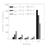
Figure 23: Number of A104 survey field galaxies (excluding galaxies in the A104 cluster itself) as a function of the number of group members for friends–of–friends analyses with three pairs of parameters: dark gray, $l_{\rm trans}=0.7$, $l_{\rm z}=500$ km s^-1; medium gray, $l_{\rm trans}=0.5$, $l_{\rm z}=350$ km s^-1; and light gray, $l_{\rm trans}=0.2$, $l_{\rm z}=350$ km s^-1).

The results of our friends–of–friends analysis for the A104 survey field, with A104 itself excluded, are plotted in Figure 23. For three different combinations of line–of–sight and transverse linking parameters, we show the number of galaxies in groups of multiplicity 1 (i.e., isolated galaxies), 2, 3, 4, and $\geq 5$. As expected, the general trend in the plot is that, as the density threshold is raised, fewer galaxies reside in large clumps and more galaxies are found in small groups or are entirely isolated. It is also striking, however, how large a fraction of galaxies are part of groups with five or more members. At our lowest overdensity threshold, $\sim 5$, 87% of galaxies have five or more linked companions, and this fraction only declines to approximately 50% at an overdensity threshold of $\sim 250$. It is important to interpret these numbers cautiously due to the sensitivity of the results to the precise value of the linking parameter, the uncertainties involved with the redshift–space distortions, and the only approximate relationship between the linking parameter and overdensity threshold. Nevertheless, these results do support our visual impressions of the galaxy distribution displayed in Figure 22. As a further illustration that the friends–of–friends of analysis is identifying credible galaxy structures (at an overdensity of $\sim 5$), we replot in Figures 24 and 25, which are projections over declination and right ascension, respectively, the galaxy distribution shown in Figure 22 but with all the galaxies in a given group marked in the same color. Aside from occasional illusions caused by the projections over one dimension, there is no doubt that the friends–of–friends analysis is finding plausible galaxy structures.

We have also applied a friends–of–friends analysis to dark matter halos identified in $N$–body simulations and will discuss the results in §7.2.

7 Discussion and Conclusions

We have presented an analysis of the clustering, pairwise velocity dispersion, and large–scale structure in two independent redshift surveys of field galaxies at intermediate redshifts ($0.2<z<0.5$). Our combined survey sparsely covers a very large region ($\sim 20$ sq. deg.) and includes redshifts for 835 galaxies with $r\leq 21$ mag and $0.2<z<0.5$. The large area reduces the errors due to cosmic variance down to levels comparable to the statistical errors (i.e., at $1h^{-1}$ Mpc, $\lesssim 10$% for the correlation strength and $\lesssim 20$% for the pairwise velocity dispersion), providing a firm foundation for analyzing the evolution of clustering and the pairwise velocity dispersion.

7.1 Redshift Evolution of $\xi$ and $\sigma_{12}$

Assuming that $\xi(r,z)$ is well fit by a power-law $(r/r_{0})^{-\gamma}$, it has been customary to parameterize the evolution of $\xi(r,z)$ with a power law (Groth & Peebles 1977):

$$\xi(r,z)=\xi(r,0)(1+z)^{-(3+\epsilon-\gamma)}\,,$$ (14)

where $r$ is the comoving separation. For clustering which is fixed in comoving coordinates, the evolutionary parameter $\epsilon=\gamma-3$. For clustering which is fixed in physical coordinates, $\epsilon=0$. Linear theory applied to the matter distribution predicts $\epsilon=\gamma-1$ (Peebles 1980). The comoving correlation length can be written as

$$r_{0}(z)=r_{0}(z=0)(1+z)^{-(3+\epsilon-\gamma)/\gamma}.$$ (15)

It is likely that this prescription is too simplistic. First, the linear theory prescription only applies to the mass distribution. In cold dark matter scenarios, galaxies form in dark matter halos, and so one should compare the measured clustering of galaxies with the clustering of halos. Second, galaxies may form in halos only in a biased fashion, and this bias may change with redshift. $N$-body simulations demonstrate that the Groth & Peebles model is not accurate (Colin et al. 1997; Ma 1999). The evolution of $\xi$ for halos is substantially slower that the evolution of $\xi$ for matter, and its redshift dependence is not well–described by the power-law model given in Equation 14.

In Figure 26, we plot an assortment of measurements of the comoving correlation length as a function of redshift. Low redshift data come from the combined CfA2/SSRS2 survey (Marzke et al. 1995), the Stromlo/APM survey (Loveday et al. 1995), the Las Campanas Redshift Survey (Jing et al. 1998), and the infrared–selected 1.2 Jy IRAS survey (Fisher et al. 1994). At high redshifts, we plot the measurements presented here, the $z=0.37$ point from the CNOCI survey (Shepherd et al. 1997); the $z=0.08$, $z=0.14$, $z=0.28$, and $z=0.43$ points from the CNOCII survey (Carlberg et al. 1999); the $z=0.34$, $z=0.62$, and $z=0.86$ points from the CFRS survey (Le Fèvre et al. 1996); and the $z=0.5$ estimate obtained by Postman et al. (1998) by deprojecting their wide–field $I$-band imaging data. For ease of comparison with previous work, the points plotted here are for $q_{0}=0.1$ (or $q_{0}=0$). Note that the three solid squares marking our measurements for the Abell 104 field are not independent. The low redshift point is for galaxies in the redshift interval $0.2<z<0.3$, the high redshift point is for galaxies in the redshift interval $0.3<z<0.5$, and the point in between is for galaxies in the combined redshift interval $0.2<z<0.5$. Although there is a wide dispersion in the measurement of $r_{0}$ at all redshifts, there is a strong indication that the comoving correlation length declines slowly beyond $z\approx 0$. The pioneering CFRS survey suggests the most dramatic decline in the correlation length. The CFRS results, however, should be interpreted with caution since the survey covered such a small volume and includes mainly sub–$L^{\ast}$ galaxies at $z\lesssim 0.5$. The CNOCI measurement is also low, but it too may suffer from cosmic variance caused by analyzing only a small volume. The results from the larger volumes surveyed by CNOCII, Postman et al. (1998), and ourselves are all consistently above the CFRS and CNOCI points and suggest a more modest decline in the comoving correlation length with redshift.

As an illustration, we also plot in Figure 26 estimates of the comoving correlation length for dark matter halos with masses greater than $2.5\times 10^{12}$ M_⊙ from the $N$–body simulations presented in Ma (1999). Results for three cosmological models are shown: the standard $\Omega_{m}=1$ cold dark matter model with $\sigma_{8}=0.7$ and two low-density models with a cosmological constant, $(\Omega_{m},\Omega_{\Lambda})=(0.5,0.5)$ and (0.3, 0.7), normalized to COBE. For each model, we have only plotted the correlation length at one redshift because the variation of the comoving correlation length is less than 10% over the entire redshift range from $z=0$ to $z=1.5$. The correlation length at $z\sim 0.4$ has a clear dependence on the matter density parameter $\Omega_{m}$. The models with lower $\Omega_{m}$ have larger $r_{0}$ because the universe is dominated by the vacuum energy at this low redshift and gravitational clustering has effectively stopped. However, it should be remembered that the correlation length depends on the halo population, and there may exist a nontrivial relationship between the dark matter halo distribution in simulations and the observed galaxy distribution. Recent work has proposed ways to make connections between halo and galaxy distributions by combining semi–analytic models of galaxy evolution with traditional $N$-body simulations (Kauffmann et al. 1999, 1998; Baugh et al. 1998). While the uncertainties associated with these semi–analytic models are still large, the models can produce plausible galaxy evolution histories and can match many observed properties of the evolving galaxy population from $z\sim 3$ to the present. The details of the predicted clustering evolution depend on a large number of factors, including the cosmological model, the nature of the dark matter, the type of galaxies observed, the waveband of the observations, and so on. The sensitive dependence of correlation functions on sample selection obviates—for the time being—the use of measurements of the evolution of clustering to constrain cosmological parameters. However, as emphasized by Kauffmann et al. (1998), this same sensitivity makes studies of clustering evolution a powerful tool for constraining models of galaxy formation and evolution.

Given the uncertainties in the observations and model predictions, it appears premature to attempt to draw any firm conclusions about cosmological parameters or galaxy evolution from the data presented in Figure 26. It is nonetheless worthwhile to highlight the general agreement between the data and the predictions of hierarchical structure formation models. While the clustering of the underlying matter distribution declines monotonically with increasing redshift, the comoving correlation length of galaxies is predicted to decline modestly or, in fact, remain flat until $z\sim 1.5$ and then rise at very high redshifts as the only galaxies bright enough to be observable with current instrumentation become very highly biased (Kauffmann et al. 1998, Baugh et al. 1998). The data collected in Figure 26, excluding the unusually low results from the CFRS and CNOCI surveys, show only a $1-2h^{-1}$ Mpc decline in comoving correlation length to $z\sim 0.5$. At high redshifts beyond the redshift range plotted in Figure 26, the correlation length of $z\sim 3$ Lyman–break galaxies is roughly comparable to that of local $L^{\ast}$ galaxies (Steidel et al. 1998, Giavalisco et al. 1998, Adelberger et al. 1998). Thus, the observed evolution of the galaxy correlation function broadly matches that expected in hierarchical structure formation models. Furthermore, the observed variation of the correlation length with galaxy population at a given redshift is in accord with expectations from semi–analytic models. For example, Kauffmann et al.’s models naturally explain the weaker clustering of blue and less luminous galaxies relative to red and more luminous galaxies as reflections of the typical masses of the dark halos in which different galaxies reside (i.e., blue and less luminous galaxies reside in less massive, and therefore less biased, halos than red and more luminous galaxies). As both the observations and the theoretical models are refined, it is clear that studies of the evolution of galaxy clustering will provide valuable insights into galaxy formation and evolution.

As discussed in §5 above, the pairwise velocity dispersion $\sigma_{12}$ is a more difficult quantity to measure reliably than the spatial two–point correlation function $\xi$. Our measurement of $\sigma_{12}(r_{p}=1.24h^{-1}\rm{Mpc})=326^{+67}_{-52}$ km s^-1 at $z_{med}=0.3$ indicates a $\sim 25$% decrease from the typical values measured locally, although our value is comparable to the pairwise velocity dispersion of local samples selected in the infrared or with early–type galaxies or clusters excluded. Preliminary results from CNOCII are consistent with our finding.

7.2 Very Large Scale Structure

The map of the large–scale galaxy distribution out to $z=0.5$ in the Abell 104 field presented in Figures 24 and 25 exhibits a striking structure in which the galaxies lie mainly in thin sheets surrounding large ($\sim 50-60h^{-1}$ Mpc), nearly empty voids, similar to the pattern of structure seen in local surveys. Using a friends–of–friends analysis, we found that only $\sim 10$% of galaxies in the survey did not lie in a structure with an overdensity of at least $\sim 5$. We have also performed a real–space friends–of–friends analysis of the halos formed in the $N$–body simulations described in the previous section. Although the precise numbers depend very sensitively on the linking parameter chosen and the minimum mass of the selected halos, the results from the $N$–body simulations are compatible with the observations. For example, the percentage of halos with masses greater than $10^{12}$ M_⊙ which are part of larger structures with overdensities $\gtrsim 5$ ($l\approx 0.7$) is approximately 80% for the standard cold dark matter model and 70% for the $(\Omega_{m},\Omega_{\Lambda})=(0.3,0.7)$ model. As an illustration of the sensitivity of these numbers to the chosen parameters, we note that 100% of the $10^{12}$ M_⊙ and greater halos are linked together in the low–density model when the linking parameter is raised to $l\approx 0.9$.

The pattern of sheets and shells visible in the galaxy distribution, if fortuitously aligned along the line of sight, could be responsible for the apparent $128h^{-1}$ Mpc periodicity observed by Broadhurst et al. (1990) in their pencil–beam survey of the North and South Galactic poles. This pattern is probably also reflected in the prominent redshift–space spikes observed by Cohen et al. (1996) in their K–band–selected redshift survey. However, as emphasized by Kaiser & Peacock (1991), the appearance of periodic structures in pencil–beam redshifts surveys is exaggerated by projection of small–scale power in the three–dimensional power spectrum to large scales in the one–dimensional power spectrum. Nevertheless, there remain credible detections of excess power on $\sim 100h^{-1}$ Mpc scales, particularly in the two–dimensional power spectrum of galaxies in the Las Campanas Redshift Survey (Landy et al. 1996) and in the distibution of rich clusters of galaxies (Einasto 1998). We are, therefore, continuing our survey in the Corona Borealis region in order to be able to compute the three–dimensional power spectrum at $z_{med}\approx 0.3$ and to delineate structure on transverse scales of $\sim 100h^{-1}$ Mpc at $z\sim 0.5$. Additional data will, of course, also allow improved estimates of the intermediate–redshift correlation function and pairwise velocity dispersion.

Table 1: Best–Fit Power–Law Correlation Function Parameters

Sample	Redshift Range	$N_{\rm gal}$	$z_{\rm med}$	$r_{0}$ ($h^{-1}$ Mpc)		$\gamma$
				$q_{0}=0.1$	$q_{0}=0.5$
Abell 104 Survey Field
all galaxies	$0.2<z\leq 0.5$	558	0.30	$4.02\pm 0.14$	$3.70\pm 0.13$	$1.77\pm 0.05$
$W_{0}[$O II] $<$ 10Å	$0.2<z\leq 0.5$	349	0.31	$4.46\pm 0.19$	$4.16\pm 0.18$	$1.84\pm 0.07$
$W_{0}[$O II] $>$ 10Å	$0.2<z\leq 0.5$	201	0.29	$3.80\pm 0.40$	$3.38\pm 0.37$	$1.85\pm 0.18$
all galaxies	$0.2<z\leq 0.3$	275	0.25	$3.96\pm 0.19$	$3.70\pm 0.19$	$1.75\pm 0.06$
$M(B_{AB})<M^{\ast}$	$0.2<z\leq 0.3$	99	0.25	$4.34\pm 0.38$	$4.09\pm 0.37$	$1.99\pm 0.14$
$M(B_{AB})>M^{\ast}$	$0.2<z\leq 0.3$	175	0.25	$3.84\pm 0.27$	$3.50\pm 0.27$	$1.73\pm 0.10$
all galaxies	$0.3<z\leq 0.5$	283	0.38	$4.80\pm 0.30$	$4.26\pm 0.25$	$1.68\pm 0.08$
all galaxies	$0.32<z\leq 0.5$	212	0.39	$4.16\pm 0.35$	$3.78\pm 0.32$	$1.72\pm 0.12$
Corona Borealis Survey Field
all galaxies	$0.2<z\leq 0.5$	277	0.29	$4.26\pm 0.42$	$3.92\pm 0.35$	$1.63\pm 0.10$

Table 2: Rest–Frame Pairwise Velocity Dispersion at $z_{\rm med}=0.30$

	Abell 104 Field	Corona Borealis Field
$r_{p}$	$\sigma_{12}$	$\sigma_{12}$
($h^{-1}$ Mpc)	(km s-1)	(km s-1)
0.14	$292^{+91}_{-80}$	$\cdots$
0.29	$329^{+119}_{-94}$	$\cdots$
0.60	$368^{+105}_{-74}$	$312^{+248}_{-141}$
1.24	$326^{+67}_{-52}$	$357^{+271}_{-144}$
2.57	$192^{+44}_{-37}$	$\cdots$
5.34	$143^{+78}_{-69}$	$\cdots$
11.11	$57^{+205}_{-43}$	$\cdots$

Note. — All fits hold $F\equiv 1$, which corresponds to assuming that the stable clustering hypothesis is correct and applies on the scales probed here. Our estimates of $\sigma_{12}$ only weakly depend on this assumption.

Figure 1: Location on the sky of all 981 $r<21$ mag galaxies with measured redshifts in the Corona Borealis survey fields included in this paper. Galaxies plotted with filled circles have $z>0.2$, while galaxies plotted with unfilled circles have $z<0.2$. The large circles mark the positions of the cataloged Abell clusters in the field. Clusters whose names are underlined lie within the Corona Borealis supercluster ($z\approx 0.07$).

Figure 2: Redshift histogram of $r<21$ mag galaxies in the Corona Borealis fields included in this paper. The two prominent peaks, one at $z\approx 0.07$ and the other at $z\approx 0.11$, are the Corona Borealis supercluster and the A2609 supercluster, respectively. (See Small et al. [1998] for a detailed analysis of the superclusters.)

Figure 3: Histogram of the ratio of the number of galaxies with measured redshifts to the total number of galaxies in the survey fields as a function of magnitude, $s_{m}(m)$.

Figure 4: Spatial selection function for the Corona Borealis field. The gray scale, ranging from 0. to 2.0, shows the fraction of galaxies successfully identified in each $3^{\prime}\times 3^{\prime}$ area of the survey field, normalized by the fraction of galaxies identified in the entire survey. The contours are drawn at 0.5, 1.0, and 1.5. For clarity, we have applied a Gaussian smoothing filter with $\sigma=1$′.

Figure 5: Ratio of number of pairs of galaxies successfully observed to the number of pairs of galaxies in the catalog selected according to the combined (magnitude times geometrical) selection function of the survey. The inset plot shows an expanded view for separations from 0 to 180 arcsec.

Figure 6: Plot of all galaxies in the Abell 104 survey field with $r<21$ mag. Galaxies plotted with filled circles have $z>0.2$, while galaxies plotted with unfilled circles have $z<0.2$. The Abell 104 cluster is located at the center of the plot.

Figure 7: Histogram of the ratio of the number of galaxies with measured redshifts to the total number of galaxies in the field as a function of magnitude, $s_{m}(m)$.

Figure 8: Redshift histogram of galaxies in the Abell 104 survey field with $r<21$ mag. The prominent peak at $z\approx 0.08$ is the Abell 104 cluster of galaxies.

Figure 9: Spatial selection function for the Abell 104 field. The gray scale, ranging from 0. to 2.0, shows the fraction of galaxies successfully identified in each $3^{\prime}\times 3^{\prime}$ area of the survey field. The contours are drawn at 0.50, 1.0, and 1.5.

Figure 10: Ratio of number of pairs of galaxies successfully observed to the number of pairs of galaxies in the catalog selected according to the combined (magnitude plus spatial) selection function of the survey. The inset plot shows an expanded view for separations from 0 to 180 arcsec.

Figure 11: Angular correlation function of the galaxies with measured redshifts in the Corona Borealis and Abell 104 survey fields (top and bottom panels, respectively), both with and without correction for missing pairs on small scales ($\leq 600$″ for Corona Borealis and $\leq 200$″ for Abell 104; filled triangles and squares, respectively), compared with that of all the galaxies in the survey field (unfilled circles). With the correction for missing pairs, the angular correlation functions of the galaxies with measured redshifts agree well with the angular correlation functions of all the galaxies in the surveys.

Figure 12: Smoothed contour plots of $\xi(r_{p},r_{\pi})$ for Abell 104 (top panel) and Corona Borealis (bottom panel) galaxies with $0.2\leq z\leq 0.5$. The contour levels are described in the text. The elongation of the contours at small $r_{p}$ is due to the velocity dispersion of bound paris. The flattening of the contours for $5h^{-1}\rm{Mpc}\lesssim{r_{p}}\lesssim 10h^{-1}\rm{Mpc}$ is due to coherent motions. For the Abell 104 survey, $\xi(r_{p},r_{\pi})$ is dominated by only a few structures and is very unlikely to be representative of the universe as a whole for $r_{p}\gtrsim 10h^{-1}$ Mpc.

Figure 13: $w_{p}(r_{p})$ for $0.2\leq z\leq 0.5$ for the Abell 104 survey (unfilled squares) and the Corona Borealis survey (filled squares). Also shown are power–law fits to the correlation functions computed for the CFRS (solid line) and CNOC1 (dashed line) surveys, local optically–selected surveys (upper dash–dotted line), the 1.2 Jy $IRAS$ Galaxy Redshift survey (lower dash–dotted line), and the best fit to the Abell 104 survey data (dotted line).

Figure 14: Error contours of $(r_{0},\gamma)$ for power–law fits to the projected two–point correlation functions of galaxies with $0.2<z<0.5$ in the Abell 104 (solid contours) and Corona Borealis (dashed contours) fields. The contour levels correspond to 1$\sigma$ on the parameters taken individually, 1$\sigma$ on the parameters taken jointly, 2$\sigma$ on the parameters taken jointly, and 3$\sigma$ on the parameters taken individually. Also plotted are the values of $r_{0}$ and $\gamma$ from the CFRS survey (with $\gamma$ held fixed at 1.64), the CNOCI survey (with $\gamma$ held fixed at 1.70), and the Las Campanas Redshift survey.

Figure 15: The projected correlation function of galaxy samples from the Abell 104 survey with $0.2<z<0.3$ (filled squares), $0.3<z<0.5$ (filled circles), $0.32<z<0.5$ (filled stars), and $0.2<z<0.5$ (unfilled squares)

Figure 16: Error contours of $(r_{0},\gamma)$ for power–law fits to the projected correlation functions for samples selected from different redshift intervals ($0.2<z\leq 0.3$, solid contours; $0.3<z\leq 0.5$, dashed contours; $0.2<z<0.5$, dot–dashed contours) from the Abell 104 survey. The contour levels are the same as in Figure 14. Within the errors, there is no evidence within our survey for variation of either $r_{0}$ or $\gamma$ with redshift.

Figure 17: $w_{p}(r_{p})$ divided by $W_{0}[$O II] for $0.2\leq z\leq 0.5$ for the Abell 104 survey. Galaxies with $W_{0}[$O II] $>10$Å are marked with filled stars, and galaxies with $W_{0}[$O II] $<10$Å are marked with filled squares. For comparison, $w_{p}(r_{p})$ for the whole sample is plotted with filled circles.

Figure 18: Error contours of $(r_{0},\gamma)$ for power–law fits to the projected two–point correlation functions of actively star–forming ($W_{0}[$O II] $>10$Å  dashed contours) and quiescent ($W_{0}[$O II] $<10$Å  solid contours) galaxies with $0.2<z<0.5$ in the Abell 104 field. The contour levels are the same as in Figure 14.

Figure 19: $w_{p}(r_{p})$ divided by M($B_{AB}$) for $0.2\leq z\leq 0.3$ for the Abell 104 survey. $w_{p}(r_{p})$ for intrinsically luminous galaxies with M($B_{AB}$) $\leq-19.45+5\log h$ is plotted with filled squares, and $w_{p}(r_{p})$ for intrinsically faint galaxies with M($B_{AB}$) $\geq-19.45+5\log h$ is plotted with filled stars. The solid line shows the best power–law fit to the projected correlation function of $0.2\leq z\leq 0.3$ galaxies in the A104 field. We have neglected the very low point at $r_{p}=5.3h^{-1}$ Mpc when fitting the projected correlation function of the intrinsically faint galaxies.

Figure 20: Error contours of $(r_{0},\gamma)$ for power–law fits to the projected two–point correlation functions of intrinsically faint (dashed contours) and intrinsically bright (solid contours) galaxies with $0.2<z<0.3$ in the Abell 104 field. The contour levels are the same as in Figure 14.

Figure 21: Rest–frame $\sigma_{12}$ for the A104 survey (filled circles) and the Corona Borealis survey (unfilled circles, offset by 0.05 dex in $r_{p}$ for clarity) galaxies with $0.2\leq z\leq 0.5$ ($z_{\rm med}=0.30$) as a function of projected separation $r_{p}$. We have assumed that the stable clustering hypothesis applies (i.e., $F\equiv 1$); our estimates of of $\sigma_{12}$ are insensitive to $F$.

Figure 22: Redshift–Right–Ascension pie diagram for the A104 survey, split into five panels of $\Delta z=0.1$. The filled and unfilled circles represent galaxies dominated by an old stellar population and galaxies dominated by star formation, respectively. The prominent clump of galaxies at $z\approx 0.08$ is Abell 104. The comoving widths of the panels at $z=0.05,0.15,0.25,0.35,{\rm and}\ 0.45$ are (for $q_{0}=0.5$) 5.0, 14.1, 22.1, 29.2, and 35.5 $h^{-1}$ Mpc, respectively.

Figure 24: Redshift–Right–Ascension pie diagram for the A104 survey, split into five panels of $\Delta z=0.1$, with friends–of–friends selected structures with $\delta\rho/\rho\sim 5$ ($l_{\rm trans}=0.7$, $l_{\rm z}=500$ km s^-1) marked by the sequence of colors. The comoving widths of the panels at $z=0.05,0.15,0.25,0.35,{\rm and}\ 0.45$ are (for $q_{0}=0.5$) 5.0, 14.1, 22.1, 29.2, and 35.5 $h^{-1}$ Mpc, respectively.

Figure 25: Redshift–Declination pie diagram for the A104 survey, split into five panels of $\Delta z=0.1$, with friends–of–friends selected structures with $\delta\rho/\rho\sim 5$ ($l_{\rm trans}=0.7$, $l_{\rm z}=500$ km s^-1) marked by the sequence of colors. The comoving widths of the panels at $z=0.05,0.15,0.25,0.35,{\rm and}\ 0.45$ are (for $q_{0}=0.5$) 5.0, 14.1, 22.1, 29.2, and 35.5 $h^{-1}$ Mpc, respectively.

Figure 26: The comoving correlation length $r_{0,\rm comoving}$ as a function of redshift for a heterogeneous assortment of redshift and imaging surveys. The higher redshift points are all plotted for $q_{0}=0.1$ (or $q_{0}=0$). Also plotted are comoving correlation lengths for halos with masses larger than $2.5\times 10^{12}$ M_⊙ identified in the $N$–body simulations of Ma (1999). See text and plot legend for details.

References

- Adelberger et al. (1998) Adelberger, K., Steidel, C., Giavalisco, M., Dickinson, M., Pettini, M., & Kellogg, M. 1998, ApJ, 505, 18
- Bagla (1998) Bagla, J. 1998, MNRAS, 297, 251
- Baugh et al. (1998) Baugh, C., Benson, A., Cole, S., Frenk, C., & Lacey, C. 1998, MNRAS, submitted [astro-ph/9811222]
- Brainerd & Smail (1998) Brainerd, T. & Smail, I. 1998, ApJ, 494, L137
- Broadhurst et al. (1990) Broadhurst, T., Ellis, R., Koo, D., & Szalay, A. 1990, Nature, 343, 726
- Carlberg et al. (1997) Carlberg, R., Cowie, L., Songaila, A., & Hu, E. 1997, ApJ, 484, 538
- Carlberg et al. (1999) Carlberg, R., et al. 1999, Phil. Trans. R. Soc. Lond. A, 357, 167
- Cohen et al. (1996) Cohen, J., Hogg, D., Pahre, M., & Blandford, R. 1996, ApJ, 462, L9
- Cole et al. (1994) Cole, S., Ellis, R., Broadhurst, T., & Colless, M. 1994, MNRAS, 267, 541
- Coleman et al. (1980) Coleman, G., Wu, C.-C., & Weedman, D. 1980, ApJS, 43, 393
- Colin et al. (1997) Colín, P., Carlberg, R., & Couchman, H. 1997, ApJ, 490, 1
- Cowie et al. (1996) Cowie, L., Songaila, A., Hu, E., & Cohen, J. 1996, AJ, 112, 839
- Davis & Huchra (1982) Davis, M., & Huchra, J. 1982, ApJ, 254, 437
- Davis & Peebles (1993) Davis, M., & Peebles, P. 1983, ApJ, 267, 465
- de Lapparent et al. (1997) de Lapparent, V., Galaz, G., Arnouts, S., Bardelli, S., & Ramella, M. 1997, ESO Messenger, 89, 21
- Diaferio & Geller (1996) Diaferio, A. & Geller, M. 1996, ApJ, 467, 19
- Efstathiou et al. (1988) Efstathiou, G., Frenk, C., White, S., & Davis, M. 1988, MNRAS, 235, 715
- Einasto (1998) Einasto, J. 1998 [astro-ph/9811432]
- Ellis et al. (1996) Ellis, R., Colless, M., Broadhurst, T., Heyl, J., & Glazebrook, K. 1996, MNRAS, 280, 235
- Fisher et al. (1994) Fisher, K., Davis, M., Strauss, M., Yahil, A., & Huchra, J. 1994, MNRAS, 267, 927
- Giavalisco et al. (1998) Giavalisco, M., Steidel, C., Adelberger, K., Dickinson, M., Pettini, M., & Kellogg, M. 1998, ApJ, 503, 543
- Geller & Huchra (1989) Geller, M. & Huchra, J. 1989, Science, 246, 897
- Groth & Peebles (1977) Groth, E. & Peebles, P.J.E. 1977, ApJ, 217, 385
- Guzzo et al. (1997) Guzzo, L., Strauss, M., Fisher, K., Giovanelli, R., & Haynes, M. 1997, ApJ, 489, 37
- Hamilton (1993) Hamilton, D., Oke, J., Carr, M., Cromer, J., Harris, F., Cohen, J., Emery, E., & Blakee, L. 1993, PASP, 105, 1308
- Hamilton (1998) Hamilton, A. 1998, in The Evolving Universe: Selected Topics on Large–Scale Structure and on the Properties of Galaxies, ed. D. Hamilton (Dordrecht: Kluwer), 185
- Huchra & Geller (1982) Huchra, J., & Geller, M. 1982, ApJ, 257, 423
- Jing et al. (1998) Jing, Y., Mo, H., & Börner, G. 1998, ApJ, 494, 1
- (29) Jing, Y., & Börner, G. 1998, ApJ, 503, 502
- Juszkiewicz et al. (1998) Juszkiewicz, R., Fisher, K., & Szapudi, I. 1998, ApJ, 504, L1
- (31) Kaiser, N. & Peacock, J. 1991, ApJ, 379, 482
- Kauffmann et al. (1998) Kauffmann, G., Colberg, J., Diaferio, A., & White, S. 1998, MNRAS, submitted [astro-ph/9809168]
- (33) Kauffmann, G., Colberg, J., Diaferio, A., & White, S. 1999, MNRAS, 303, 188
- Kennicutt (1992) Kennicutt, R. 1992, ApJ, 388, 310
- Landy & Szalay (1993) Landy, S., & Szalay, A. 1993, ApJ, 412, 64
- Landy et al. (1996) Landy, S., Shectman, S., Lin, H., Kirshner, R., Oemler, A., & Tucker, D. 1996, ApJ, 456, L1
- Landy et al. (1998) Landy, S., Szalay, A., & Broadhurst, T. 1998, ApJ, 494, L133
- Le Fevre et al. (1996) Le Fèvre, O., Hudon, D., Lilly, S., Crampton, D., Hammer, F., & Tresse, L. 1996, ApJ, 461, 534
- (39) Lilly, S., Le Fèvre, O., Crampton, D., Hammer, F., & Tresse, L. 1995, ApJ, 455, 50
- (40) Lilly, S., Tresse, L., Hammer, F., Crampton, D., & Le Fèvre, O. 1995, ApJ, 455, 108
- Lin et al. (1998) Lin, H. et al. 1998, in The Young Universe, ed. S. D’Odorico, A. Fontana, & E. Giallongo (San Francisco: ASP), p. 190
- Ling et al. (1986) Ling, E., Barrow, J., & Frenk, C. 1986, MNRAS, 223, P21
- Loveday et al. (1995) Loveday, J., Maddox, S., Efstathiou, G., & Peterson, B. 1995, ApJ, 442, 457
- Ma (1998) Ma, C.-P. 1999, ApJ, 510, 32
- Marzke et al. (1995) Marzke, R., Geller, M., Da Costa, L., & Huchra, J. 1995, AJ, 110, 477
- Mo et al. (1993) Mo, H., Jing, Y., & Börner, G. 1993, MNRAS, 264, 825
- Nolthenius & White (1987) Nolthenius, R., & White, S. 1987, MNRAS, 235, 505
- Peebles (1980) Peebles, P.J.E. 1980 Large–Scale Structure in the Universe (Princeton: Princeton University Press)
- Postman et al. (1998) Postman, M., Lauer, T., Szapudi, I., & Oegerle, W. 1998, ApJ, 506, 33
- Ratcliffe et al. (1998) Ratcliffe, A., Shanks, T., Parker, Q., & Fong, R. 1998, MNRAS, 296, 191
- Reid et al. (1991) Reid, I., et al. 1991, PASP, 331, 465
- Sargent & Turner (1977) Sargent, W., & Turner, E. 1977, ApJ, 212, L3
- Schechter (1976) Schechter, P. 1976, ApJ, 203, 297
- Shepherd et al. (1997) Shepherd, C., Carlberg, R., Yee, H., & Ellingson, E. 1997, ApJ, 479, 82
- Sheth (1996) Sheth, R. 1996, MNRAS, 279, 1310
- (56) Small, T., Sargent, W., & Hamilton, D. 1997a, ApJS, 111, 1
- (57) Small, T., Sargent, W., & Hamilton, D. 1997b, ApJ, 487, 512
- Small et al. (1998) Small, T., Ma, C.-P., Sargent, W., & Hamilton, D. 1998, ApJ, 492, 45
- Small et al. (1999) Small, T., Sargent, W., & Hamilton, D. 1999, in preparation
- Steidel et al. (1998) Steidel, C., Adelberger, K., Dickinson, M., Giavalisco, M., Pettini, M., & Kellogg, M. 1998, ApJ, 492, 428
- Somerville et al. (1997) Somerville, R., Davis, M., & Primack, J. 1997, ApJ, 479, 616
- Tucker et al. (1997) Tucker, D., et al. 1997, MNRAS, 285, L5
- Yee, Ellingson, & Carlberg (1996) Yee, H., Ellingson, E., & Carlberg, R. 1996, ApJS, 102, 269
- Zurek et al. (1994) Zurek, W., Quinn, P., Salmon, J., & Warren, M. 1994, ApJ, 431, 559