Ray Tracing Simulations of Weak Lensing by Large-Scale Structure

Abstract

We investigate weak lensing by large-scale structure using ray tracing through N-body simulations. Photon trajectories are followed through high resolution simulations of structure formation to make simulated maps of shear and convergence on the sky. Tests with varying numerical parameters are used to calibrate the accuracy of computed lensing statistics on angular scales from $\sim$ 1 arcminute to a few degrees. Various aspects of the weak lensing approximation are also tested. We show that the non-scalar component of the shear generated by the multiple deflections is small. For fields a few degrees on a side the shear power spectrum is almost entirely in the nonlinear regime and agrees well with nonlinear analytical predictions. Sampling fluctuations in power spectrum estimates are investigated by comparing several ray tracing realizations of a given model. For survey areas smaller than a degree on a side the main source of scatter is nonlinear coupling to modes larger than the survey. We develop a method which uses this effect to estimate $\Omega_{\rm m}$ from the scatter in power spectrum estimates for subregions of a larger survey. We show that the power spectrum can be measured accurately on scales corresponding to $1-10\,h^{-1}$Mpc with realistic number densities of source galaxies with large intrinsic ellipticities. Non-Gaussian features in the one point distribution function of the weak lensing convergence (reconstructed from the shear) are also sensitive to $\Omega_{\rm m}$. We suggest several techniques for estimating $\Omega_{\rm m}$ in the presence of noise and compare their statistical power, robustness and simplicity. With realistic number densities of source galaxies $\Omega_{\rm m}$ can be determined to within $0.1-0.2$ from a deep survey of several square degrees.

1 Introduction

Mapping the large-scale structure (LSS) of the universe is one of the major goals of observational cosmology. Traditionally this is performed using large surveys of galaxies. Such surveys map the light distribution, while most of the matter in the universe appears to be dark. This paper focuses on mapping the dark matter using gravitational lensing, in particular, weak lensing of distant background galaxies by large-scale structure. Weak lensing magnifies and shears the images of these galaxies, inducing an additional ellipticity which, although not detectable in any individual image, can be measured as a function of position on the sky by averaging the ellipticities of neighboring galaxies. This observable is determined by a line-of-sight projection of the mass fluctuations and by the spatial geometry of the universe. When averaged over windows of arcminute scale, the ellipticities of distant galaxies probe mass fluctuations on scales of 1-10 $h^{-1}$ Mpc. If the shape of the mass fluctuation spectrum is known, such measures are sensitive to the cosmological parameters $\Omega_{\rm m}$ and $\Omega_{\Lambda}$. Thus while strong lensing leads to highly distorted or multiple images and probes the densest regions of the universe, the inner cores of massive halos, weak lensing provides a direct measure of typical mass fluctuations on larger scales.

Observatonal attempts at detection of weak lensing by large-scale structure include the work of Fahlman et al. (1994), Mould et al. (1994), Refregier et al. (1998) and Schneider et al. (1998). While a definitive detection has yet to be made, a few groups have demonstrated the capability to measure the small shear signal induced by large-scale structure. Kaiser et al. (1998) have made a convincing detection of coherent shear due to a supercluster. Several observational efforts to measure weak lensing that use wide field CCD detectors are currently underway (see Mellier 1998 for a review).

The first weak lensing calculations to use modern models for the large-scale matter distribution were those of Blandford et al. (1991); Miralda-Escude (1991) and Kaiser (1992), based on the pioneering work of Gunn (1967). More recently, Villumsen (1996), Stebbins (1996), Bernardeau et al (1997) and Kaiser (1998) have made linear calculations for a variety of cosmologies, while Jain & Seljak (1997) have included the effect of the nonlinear evolution of the matter power spectrum. Numerical simulations of gravitational lensing have also been developed in parallel. Different approximations have been used to represent the lumpy distribution of dark matter, typically in conjunction with methods which trace rays through a series of lens planes (Schneider & Weiss 1988; Jaroszyński et al 1990; Lee & Paczyński 1990; Jaroszyński 1991; Babul & Lee 1991; Bartelmann & Schneider 1991; Blandford et al. 1991). The most detailed numerical study of lensing by large-scale structure has been conducted by Wambsganss, Cen & Ostriker (1998), building on the earlier work of Wambsganss et al (1995, 1997). Their work focused on somewhat smaller scales than we consider in this paper, and as a result was unable to address some of the nonlinear mode-coupling effects we are concerned with here. Nevertheless, there is still considerable overlap with the regime we study. Other recent studies using ray tracing have been conducted by Premadi, Martel & Matzner (1998), van Waerbeke, Bernardeau & Mellier (1998), Bartelmann et al (1998) and Couchman, Barber & Thomas (1998).

In this paper we apply a newly developed numerical method to investigate a variety of statistics that can be extracted from weak lensing data. Our numerical approach is similar to that of some of the above references, in that we approximate the matter distribution between observer and source as a sequence of discrete planes (see also Bartelmann & Schneider 1991). The projected distribution on these planes is obtained from high resolution N-body simulations and is converted to deflection angle and shear matrix distributions using Fourier techniques. These can then be used to follow $\lower 2.15277pt\hbox{$\;\buildrel>\over{\sim}\;$}10^{6}$ rays from the observer back to the source plane, giving the magnification, shear and true source position in each observed direction. The magnification and shear maps are smoothed on different scales and used to construct one-point probability distribution functions and their low-order moments. The two-point correlation function provides another simple and robust statistic and, for models with Gaussian initial conditions, it contains all the fluctuation information on linear scales. We show that to reach the linear regime one must survey regions at least 10 degrees on a side. This is difficult with existing CCD cameras which typically have field diameters of $0.25^{\circ}-0.5^{\circ}$. Most of the information in the initial surveys carried out with these instruments will therefore be in the mildly to strongly nonlinear regime; in the following we discuss methods for power spectrum extraction from such data.

While nonlinear evolution may limit the information that can be extracted from a power spectrum analysis, it also leads to non-Gaussian effects that can be detected by statistics other than second moments. These effects can provide qualitatively new information because the boundary of the linear regime depends on the relative density fluctuation, $\delta({\hbox{\boldmath{$r$}}})=\rho({\hbox{\boldmath{$r$}}})/\bar{\rho}-1$, while the amplitude of the weak lensing signal is determined by a projection of the total mass fluctuation, $\bar{\rho}\delta({\hbox{\boldmath{$r$}}})$. Studies of two-point correlators cannot separate the effect of $\bar{\rho}$ from a variation in the normalization of $\delta$, but the transition to nonlinearity depends on the density contrast alone, so that the behavior of higher moments allows a separate determination of the density parameter $\Omega_{\rm m}=\bar{\rho}/\rho_{\rm crit}$ and the matter power spectrum $P_{\delta}(k)$ (Bernardeau et al. (1996); Jain & Seljak (1997)).

In this respect weak lensing maps are easier to interpret than maps of the galaxy distribution, where non-Gaussian signatures reflect both nonlinear gravitational clustering and the details of the relation between the galaxy distribution and the underlying mass distribution. Checks of the consistency of any assumed “bias” relation are certainly valuable, but they do not provide qualitatively new information on cosmological parameters; that is why dynamical measures such as streaming motion or velocity dispersion estimates are needed for galaxy surveys to provide a robust probe of $\Omega_{\rm m}$. This point is illustrated in figure 1, which compares the one point distribution functions (pdf) of the convergence $\kappa$ and the density contrast $\delta$ for open and Einstein-de Sitter universes both with CDM power spectrum shape parameter $\Gamma=0.2$. (These were made from the ray-tracing simulations discussed in §3.) The pdf’s of $\kappa$ differ substantially even when their rms values are the same. For $\delta$, on the other hand, the rms completely determines the pdf, leaving no leverage to determine $\Omega_{\rm m}$.

Figure 1: The probability distribution function (pdf) of the convergence $\kappa$ is compared with the pdf of $\delta$, the 3-dimensional density contrast. The right panel shows the pdf of $\delta$ for an open CDM model (dashed) and an Einstein-de Sitter CDM model (solid), both smoothed on a scale of 3 $h^{-1}$ Mpc. The rms density contrast in the two models is nearly identical. The left panel shows the pdf of $\kappa$ for the same two models. The thick solid curve uses the same smoothing scale as the dashed curve, 0.5 arcmin, while the thin solid curve uses a somewhat larger smoothing scale chosen to give the same rms as the dashed curve. The rms approximately determines the full pdf for $\delta$ but not for $\kappa$.

In this paper we investigate the observability of nonlinear effects in weak lensing data. We apply statistics which measure a variety of non-Gaussian signatures to simulated data. These are obtained by ray-tracing through $N$-body simulations, and sampling the resulting shear fields with realistic number densities of source galaxies. Our main goal is to see how accurately the density parameter can be estimated, given the uncertainty in other parameters, such as the shape and amplitude of the power spectrum. The main statistic we investigate is the one-point pdf of the convergence or projected matter density. It can be analyzed in many different ways, for example by using direct maximum likelihood (ML) parameter estimation, by measuring various moments, or by constructing an Edgeworth expansion. In principle ML should give the most powerful constraints, but it is somewhat cumbersome to use and it requires a suite of cosmological simulations spanning the parameter space considered. The latter two methods are simpler and can be tested against perturbation theory, but they use the information in a less optimal way. In the following, we evaluate the performance of these estimators and compare their robustness, statistical power and simplicity.

Our results on the second moment are valid for both the convergence and shear, as their second moments are identical in the weak lensing approximation and for the range of scales of interest for lensing by large-scale structure. For the skewness and the pdf, we present results for the convergence, which is not a direct observable. We demonstrate that for fields larger than a degree on a side it is possible to reconstruct the convergence from data on the ellipticities of galaxies by using the Fourier space relations between convergence and shear (equation 28). In our modeling of observational data we have included the random errors in shear measurement due to the finite number of source galaxies, each of which has a large intrinsic ellipticity. However we have not considered realistic observational noise, such as due to seeing and possibly anisotropic point spread functions – thus we are assuming ideal imaging data in this paper. These sources of observational noise can degrade the signal and produce systematic errors that must be carefully modeled to extract the shear signal.

The outline of our paper is as follows. In §2 the formalism for the weak lensing calculation is presented. Our N-body simulations and our ray-tracing method are described in §3, where the effective resolution of our results is estimated and is tested by varying the relevant numerical parameters. §4 gives predictions for the power spectrum and the real space 2-point correlation of the convergence for various cold dark matter (CDM) models. The scatter due to noise (primarily from the finite number and intrinsic ellipticity of the background galaxies) and to the finite survey area is estimated. §5 contains a discussion of various measures of non-Gaussianity. Results for the probability distribution function and its moments are presented in §6, where we also discuss the survey size needed for an accurate measurement of $\Omega_{\rm m}$ given realistic number densities of source galaxies. A likelihood and $\chi^{2}$ analysis of the pdf is made in §7, which also further explores robust estimators of $\Omega_{\rm m}$ based on the pdf. All our results are summarized in §8.

2 Theory of multiple plane lensing

Gravitational lensing shears and magnifies the images of distant galaxies. In this section we relate the shear and magnification to perturbations in the gravitational potential along the line of sight. We first analyze the continuous case, then present a discrete approximation to it. In the discrete case the matter distribution between the source and observer is taken to lie on a finite number $N$ of lens planes. The mapping from the image plane (the first lens plane) to the source plane is then determined by adding the deflections over all the $N$ lens planes (e.g. Schneider, Ehlers & Falco 1992).

We will work in comoving coordinates $x^{i}$ and conformal time $\tau$, in terms of which the perturbed Robertson-Walker metric is

$$ds^{2}=a^{2}(\tau)\left\{-(1+2\phi)d\tau^{2}+(1-2\phi)\gamma_{ij}dx^{i}dx^{j}\right\}.$$ (1)

The spatial part of the background metric can be written as

$$\gamma_{ij}dx^{i}dx^{j}=d\chi^{2}+r^{2}(d\theta^{2}+\sin^{2}\theta d\phi^{2}),$$

$$r(\chi)=\sin_{K}\chi\equiv\left\{\begin{array}[]{ll}K^{-1/2}\sin K^{1/2}\chi,\ K>0\\ \chi,\ K=0\\ (-K)^{-1/2}\sinh(-K)^{1/2}\chi,\ K<0\\ \end{array}\right.$$ (5)

where $K$ is the curvature term which can be expressed using the present density parameter $\Omega_{0}$ and the present Hubble parameter $H_{0}$ as $K=(\Omega_{0}-1)H_{0}^{2}=-\Omega_{K}H_{0}^{2}$. Here $a(\tau)$ is the scale factor expressed in terms of conformal time and $r(\chi)$ is the comoving angular diameter distance. The evolution of $a(\tau)$ is determined by the Friedmann equation, $da/d\tau=H_{0}(\Omega_{\rm m}a+\Omega_{\Lambda}a^{4}+\Omega_{K}a^{2})^{1/2}$, where $\Omega_{\rm m},\Omega_{\Lambda},\Omega_{K}$ are the densities of matter, vacuum energy (cosmological constant) and curvature, respectively, in units of the critical density. In addition the null geodesics satisfy to lowest order the relation $d\tau=d\chi$. The density parameter $\Omega_{0}$ can have contributions from $\Omega_{\rm m}$ or $\Omega_{\Lambda}$, $\Omega_{0}=\Omega_{\rm m}+\Omega_{\Lambda}$. The advantage of using the conformal time $\tau$ is that the metric becomes conformally Euclidean ($K=0$), 3-sphere ($K>0$) or 3-hyperboloid ($K<0$), leading to a simple geometrical description of light propagation. Note that we have adopted units such that $c=1$.

The change in a photon’s direction as it propagates is governed by the space part of the geodesic equation, which, applied to the metric of equation 1, gives $d{\vec{\alpha}}=-2\vec{\nabla}_{\perp}\phi\ d\chi$, where $\phi$ is the gravitational potential, $d{\vec{\alpha}}$ the change in photon propagation direction and the symbol $\vec{\nabla}_{\perp}$ denotes the transverse derivative. An individual deflection by $d\vec{\alpha}$ at $\chi^{\prime}$ leads to a transverse excursion at $\chi$ given by $d\vec{x}_{\perp}(\chi)=r(\chi-\chi^{\prime})d\vec{\alpha}(\chi^{\prime})$. The final position at $\chi$ is given by the unperturbed position $r(\chi)\vec{\theta}(\chi=0)$ plus the integral along the photon trajectory of the individual deflections,

$$\vec{x}_{\perp}(\chi)=-2\int_{0}^{\chi}r(\chi-\chi^{\prime})\ \vec{\nabla}_{\perp}\phi[\chi^{\prime},\vec{x}_{\perp}(\chi^{\prime})]\ d\chi^{\prime}+r(\chi)\,\vec{\theta}(\chi=0).$$ (6)

Note that the gravitational potential has to be computed along the actual perturbed path of the photon, which we denote with radial position $\chi^{\prime}$ and transverse position $\vec{x}_{\perp}(\chi^{\prime})$. The angular direction at $\chi$ is given by

$$\vec{\theta}(\chi)={-2\over r({\chi})}\int_{0}^{\chi}r(\chi-\chi^{\prime})\ \vec{\nabla}_{\perp}\phi[\chi^{\prime},r(\chi^{\prime})\vec{\theta}(\chi^{\prime})]\ d\chi^{\prime}+\vec{\theta}(\chi=0).$$ (7)

From the above we define the shear matrix as

$$\Phi_{ij} \equiv {\partial\theta_{i}(\chi)\over\partial\theta_{j}(0)}-\delta_{ij}=-2\int_{0}^{\chi}g(\chi^{\prime},\chi)\ \nabla_{i}\nabla_{j}\phi[\chi^{\prime},r(\chi^{\prime})\vec{\theta}(\chi^{\prime})]\ d\chi^{\prime}\ ,$$

$$g(\chi^{\prime},\chi) = {r(\chi^{\prime})r(\chi-\chi^{\prime})\over r(\chi)}\ ,$$ (8)

where the indices $i,j$ take values $1,2$ and denote components on the sky.

The convergence of the mapping is defined as $2\kappa=\Phi_{11}+\Phi_{22}$. The two components of the shear $\hbox{\boldmath{$\gamma$}}=\gamma_{1}+i\gamma_{2}$ are similarly defined by: $2\gamma_{1}=\Phi_{11}-\Phi_{22}\ ;\ \gamma_{2}=\Phi_{12}\,.$ To obtain $\kappa$ one needs to compute $\int_{0}^{\chi}g(\nabla_{11}+\nabla_{22})\phi\,d\chi^{\prime}$ along the photon trajectory. This integral can be simplified by using the projected density distribution. The relation between the gravitational potential $\phi$ and density perturbation $\delta$ is given by Poisson’s equation

$$\nabla^{2}\phi={3H_{0}^{2}\over 2}\ \Omega_{\rm m}\ {\delta\over a}\ .$$ (9)

Using this equation the expression for $\kappa$ in terms of $\Phi_{11}$ and $\Phi_{22}$ becomes

$$\kappa=\int_{0}^{\chi}g[\nabla^{2}-\nabla_{\chi}^{2}]\phi\ d\chi^{\prime}=\int_{0}^{\chi}{3H_{0}^{2}\over 2}\ \Omega_{\rm m}\ g{\delta\over a}\ d\chi^{\prime}-\int_{0}^{\chi}g\nabla_{\chi}^{2}\phi\ d\chi^{\prime}.$$ (10)

The second term in equation (10) can be integrated by parts,

$$\int_{0}^{\chi}g\nabla_{\chi}^{2}\phi\ d\chi^{\prime}=g\nabla_{\chi}\phi|_{0}^{\chi}-\int_{0}^{\chi}[g\dot{\nabla}_{\chi}\phi+g^{\prime}\nabla_{\chi}\phi]\ d\chi^{\prime}.$$ (11)

The prime and dot denote derivatives with respect to the radial coordinate $\chi$ and conformal time $\tau$, respectively. Note that we are integrating along photon geodesics and hence $d/d\chi=\partial/\partial\tau+\partial/\partial\chi$. The boundary terms vanish because $g=0$ at $\chi^{\prime}=0$ and at $\chi^{\prime}=\chi$. The time derivative of $\nabla_{\chi}$ typically changes by order unity over the Hubble time and the term is comparable to $g^{\prime}\nabla_{\chi}\sim\nabla_{\chi}$. These two terms have to be compared to $g\nabla^{2}_{\perp}\sim\chi\nabla^{2}_{\perp}$. On small angular scales the dominant contribution to the deflections comes from scales much smaller than $\chi$, which is comparable to the Hubble length. Hence $\nabla_{\perp}^{2}\gg\nabla_{\chi}/\chi$ and the second term in equation (10) can be ignored compared to the first term everywhere except on the largest angular scales. The convergence can therefore be expressed as a projection of the density perturbation $\delta$

$$\kappa={3H_{0}^{2}\over 2}\ \Omega_{\rm m}\ \int_{0}^{\chi}g\ {\delta\over a}\ d\chi^{\prime}.$$ (12)

We will discuss other components of $\Phi$ in the following subsection.

The power spectrum of the convergence on angular wavenumber $l$ can be expressed in terms of the density power spectrum using equation (12). The result for the dimensionless power which gives the contribution to the variance per log interval in $l$ is (Jain & Seljak 1997)

$$\sigma^{2}(l)\ \equiv\ 2\pi l^{2}P(l)=36\pi^{2}\Omega_{m}^{2}l^{2}\int_{0}^{\chi}\frac{g^{2}}{r^{2}}\ \frac{P_{\delta}(k,\chi^{\prime})}{a^{2}}\ d\chi^{\prime},$$ (13)

where $P_{\delta}(k,\chi)$ is the power spectrum of the density at wavenumber $k=l/r$.

2.1 Discrete lensing approximation

We may discretize the expressions above by dividing the radial interval between source and observer into $N$ planes separated by comoving distance $\Delta\chi$. The angular position of a ray at the $n$-th plane is given by equation 7 as

$${\vec{\theta}}_{n} = \sum_{m=1}^{n-1}{r(\chi_{n}-\chi_{m})\over r(\chi_{n})}{\vec{\alpha}}_{m}+{\vec{\theta}}_{1}$$

$${\vec{\alpha}}_{m} = -2{\vec{\nabla}}_{\perp}\phi[\chi_{m},r(\chi_{m}){\vec{\theta}}_{m}]\Delta\chi\,.$$ (14)

We have assumed that the spacing between planes is sufficiently small that only the lowest order terms contribute. In analogy with the continuous case we can define the Jacobian of the mapping $\Phi_{n}$, which describes the deflections in the $n$-th plane relative to the image plane

$$\Phi_{n}={\partial{\vec{\theta}}_{n}\over\partial{\vec{\theta}}_{1}}.$$ (15)

The shear tensor in each plane $U_{m}$ is defined as

$${\partial{\vec{\alpha}}_{m}\over\partial{\vec{\theta}}_{m}}=r(\chi_{m}){\partial{\vec{\alpha}}_{m}\over\partial{\vec{x}}_{m}}=-2r(\chi_{m})\vec{\nabla}_{\perp}{\vec{\nabla}}_{\perp}\phi(r(\chi_{m}){\vec{\theta}}_{m})\Delta\chi\equiv r(\chi_{m})U_{m}\ .$$ (16)

The distortion tensor can now be written as (Schneider, Ehlers & Falco 1992; Seitz, Schneider & Ehlers 1994)

$$\Phi_{n} = {\partial{\vec{\theta}}_{n}\over\partial{\vec{\theta}}_{1}}=I+\sum_{m=1}^{n-1}{r(\chi_{n}-\chi_{m})\over r(\chi_{n})}{\partial{\vec{\alpha}}_{m}\over\partial{\vec{\theta}}_{m}}{\partial{\vec{\theta}}_{m}\over\partial{\vec{\theta}}_{1}}$$ (17)

$$= I+\sum_{m=1}^{n-1}g_{mn}U_{m}\Phi_{m},$$

where $g_{mn}=r(\chi_{n}-\chi_{m})r(\chi_{m})/r(\chi_{n})$, and $I$ denotes the identity matrix. Note that although the matrices $U_{m}$ are symmetric for all $m$, the matrices $\Phi_{m}$ are not symmetric for $m>2$. The symmetry is destroyed because the matrix products in equation 17 are not symmetric even if their component matrices are. The recursion relation in equation 17 is used by our ray-tracing code to propagate the distortion tensor. The most time-consuming computational step is the evaluation of the $U_{m}$ matrices at each photon position and on each lens plane.

In a single lens plane the 2 by 2 matrix $U_{m}$ at a given angular position is symmetric and is given by the integral of the second derivatives of the gravitational potential $\phi$ along the radial extent of the $m$-th region (equation 16). Following the discussion for the continuous case this can be approximated in terms of the projected surface density $\Sigma=\int_{\chi_{m-1}}^{\chi_{m}}\ \delta\ d\chi^{\prime}$. We define

$$K=\frac{1}{2}\left(U_{11}+U_{22}\right)={3H_{0}^{2}\over 2}\,\Omega_{\rm m}\ g\,{\Sigma\over a}\ .$$ (18)

The other two components of the symmetric tensor are

$$\Gamma_{1} = \frac{1}{2}\left(U_{11}-U_{22}\right)\ ,$$

$$\Gamma_{2} = U_{12}\ .$$ (19)

They can be obtained from $K$ using the relation between these quantities in Fourier space (which follows from the definition of $U$ in equation 16):

$$\hat{\Gamma}_{1}(\vec{l}) = \frac{l_{1}^{2}-l_{2}^{2}}{l^{2}}\hat{K}(\vec{l})\ ,$$

$$\hat{\Gamma}_{2}(\vec{l}) = \frac{2l_{1}l_{2}}{l^{2}}\hat{K}(\vec{l})\ .$$ (20)

We have used the following definition of the 2-dimensional Fourier transform of $X=K,\Gamma_{1},\Gamma_{2}$

$$X(\vec{\theta})=\int d^{2}le^{i{\vec{l}}\cdot\vec{\theta}}\hat{X}({\vec{l}})\ .$$ (21)

Finally, the shear matrix $U_{m}$ is computed at the perturbed photon positions ${\vec{\theta}}_{m}={\vec{\theta}}_{1}+\delta{\vec{\theta}}_{m}$. The perturbations $\delta{\vec{\theta}}_{m}$ can be computed from the Jacobian matrix $\Phi_{m}$ using the Fourier space relations

$$\delta\hat{\theta}_{1}=-i\hat{\Phi}_{11}/l_{1}$$

$$\delta\hat{\theta}_{2}=-i\hat{\Phi}_{22}/l_{2},$$ (22)

where we have dropped the index $m$ for clarity. One could also express the above relations in terms of off-diagonal elements of $\Phi$.

2.2 Magnification, Shear and Rotation of Galaxy Images

To obtain the ellipticity induced by gravitational lensing we consider the action of the distortion matrix $\Phi$ on a circular image. A general matrix can be decomposed into a symmetric and a rotational matrix (Schneider, Ehlers & Falco 1992)

$$\Phi=\left(\begin{array}[]{cc}\Phi_{11}&\Phi_{12}\\ \Phi_{21}&\Phi_{22}\\ \end{array}\right)\ =\left(\begin{array}[]{cc}\cos\phi&\sin\phi\\ -\sin\phi&\cos\phi\\ \end{array}\right)\ \left(\begin{array}[]{cc}1-\kappa-\gamma_{1}&-\gamma_{2}\\ -\gamma_{2}&1-\kappa+\gamma_{1}\\ \end{array}\right)\ .$$ (23)

In the symmetric case $\phi=0$ and the image of a circular source is stretched into an ellipse, with the stretch factors of the two axes given by $(1-\kappa\pm\gamma)^{-1}$, where $\gamma^{2}=\gamma_{1}^{2}+\gamma_{2}^{2}$. The direction of major axis of the ellipse is $\beta=\tan^{-1}(\gamma_{2}/\gamma_{1})/2$. The magnification of the image is given by $1/\det(\Phi)$.

If the distortion matrix $\Phi$ is not symmetric there is also an overall rotation of the image by angle $\phi$. Assuming this term is small we can expand the rotation matrix to obtain

$$\phi\approx{\Phi_{12}-\Phi_{21}\over 2(1-\kappa)}.$$ (24)

Image rotation by $\phi$ leaves the magnification unchanged to lowest order, but modifies the two shear components: $\gamma_{1}^{\prime}=\gamma_{1}+2\gamma_{2}\phi$ and $\gamma_{2}^{\prime}=\gamma_{2}-2\gamma_{1}\phi$. In general, the lowest order contributions to the rotation angle $\phi$ are quadratic in shear and are significantly smaller than the first order contributions to $\kappa$ and $\gamma$. The only situation in which rotation can be important is if two critical images that are well separated in redshift are superimposed; this is rather unlikely in our universe. We verify this below by measuring the rotational component of $\Phi$ in our simulations – it is shown in figure 7 and discussed in Section 4.

For individual galaxy images the gravitational stretching cannot be separated from the intrinsic ellipticity. However, by averaging the ellipticity of all images seen near a given direction, a smoothed version of the gravitational component can be measured. To compute the distortion in this case we need to average the distortion matrices over the smoothing window and over the redshift distribution of the sources. Let us assume we know the probability $W_{m}$ that a given galaxy lies on the $m$-th plane, where $\sum_{m}W_{m}=1$. The average distortion before angular smoothing is then

$$\Phi=\sum_{m}W_{m}\Phi_{m}\ .$$ (25)

Ray-tracing must therefore be performed up to the most distant plane where $W_{m}$ is not negligible.

3 Ray-tracing through N-body simulations

3.1 Ray-tracing procedures

The previous section contains the formulae for multiple plane lensing that we use in our ray tracing simulations. The key relations are equations (22) for the position of a given photon ${\vec{\theta}}_{n}$ and equations (17-20) for the Jacobian matrix $\Phi_{n}$ at this position. Aside from the distance factor $g_{mn}$, the main inputs into the recursion relations for ${\vec{\theta}}_{n}$ and $\Phi_{n}$ are the shear matrices $U_{m}$ and previous $\Phi_{m}$’s, all of which need to be stored.

The ray tracing algorithm consists of three parts: constructing the dark matter lens planes, computing the shear matrix on each plane, and using these to evolve the photon trajectory from the observer to the source. The details involved at each step are as follows.

1. The dark matter distribution between the source and observer is projected onto $20-30$ equally spaced lens planes, depending on the size of simulation box and the redshift of the sources. The particle dump closest in redshift to each plane is used for this projection. The projected field is a square of predetermined angular size – usually the angular size of the simulation box at the source distance. The orientation of the projection as well as the location of the origin are chosen at random. This minimizes repetition of structures from the simulation at the same projected position. The particle positions on each plane are interpolated onto a grid of size $2048^{2}$ for the P³M runs, and smaller sizes for the PM runs (the P³M and PM simulations are described in the next sub-section). The dimensionless density $K$ used in the lensing equations is given by the projected particle density times a redshift-dependent constant (see equation 18).

2. On each plane $U$ is computed on a grid. This is done by Fourier transforming the projected density $K$ and using equations (20) to obtain the shear. The inverse Fourier transform is then used to return to real space, and the shear matrix $U$ is given by linear combinations of $K$, $\Gamma_{1}$ and $\Gamma_{2}$ obtained from equations (18) and (19). Periodic boundary conditions are assumed when carrying out these operations, hence we use zero-padding to minimize the spurious effects introduced. Since the final convergence effectively depends only on a projection of the density along the photon path (equation 12) and the relative location of different planes is in any case random transverse to the line of sight, this mistreatment of the effects of the matter outside our grid has very little influence on our results.

3. The photons are started on a regular grid on the first lens plane. Perturbations along the line of sight distort this grid and are computed using equation (22). Once we have the photon positions, we interpolate the shear matrix $U$ onto them and solve equation 17 for the Jacobian matrix $\Phi_{n}$ of the mapping from the $n$-th lens plane to the first plane, using previously stored $\Phi_{m}$ and $U_{m}$.

4. Solving the recursion relations up to the source plane yields the Jacobian matrix $\Phi_{n}$ at these positions. Finally, we may sum over the redshift distribution of sources using equation 25. Note that the ray tracing is done backwards from the observer to the source, thus ensuring that all the photons reach the observer. The first lens plane is the image plane and has the unperturbed photon positions.

The use of FFT’s for computing ${\vec{\theta}}$ and $U$ simplifies and speeds up the numerical implementation. Because the CPU required for an $M^{2}$ FFT scales as $M^{2}\log M^{2}$, it is possible to use sufficiently large grids to maintain the intrinsic resolution of the N-body simulation (see below). A direct summation would be prohibitively time consuming. An alternative Poisson-solver of similar resolution would be a tree-code as used by Wambsganss et al (1995) and Wambsganss, Cen & Ostriker (1998).

We found that a substantial fraction of the overall time in a ray-tracing run was taken up by reading in the $\Sigma$ grids. The 2-dimensional FFT’s needed for computing $\vec{\alpha}$ and $U$ take the bulk of the CPU time. CPU constraints turn out, however, to be negligible: a run using grids of size $1024^{2}$ can be completed in 20-30 minutes on a DEC-alpha workstation provided it has enough memory. Memory is a problem with such large grids because the recursion relations require the storage of the $\Phi_{n}$ matrices at all the lens planes. This could be avoided if one used the recursion relation based on previous two planes only (Seitz, Schneider & Ehlers 1994), although for simplicity we have not implemented that. Thus for the 4-component matrix of real*4 numbers for the $\Phi_{n}$’s, computed on $1024^{2}$ photon positions on 20 lens planes, one needs $4\times 1024^{2}\times 20\times 4$ bytes, or about 320 Megabytes of memory. A $2048^{2}$ grid with a spatial resolution twice as good would require 4 times the memory, i.e. more than 1.2 Gigabytes – this is the grid size used for our high resolution runs.

Table 1: Parameters of the N-body simulations

Simulation	SCDM	$\tau$CDM	$\Lambda$CDM	OCDM
$N_{\rm par}$	2563	2563	2563	2563
$l_{\rm soft}[h^{-1}$ kpc]	36	36	30	30
$\Gamma$	0.5	0.21	0.21	0.21
$L_{\rm box}[h^{-1}$Mpc]	85	85	141	141
$\Omega_{0}$	1.0	1.0	0.3	0.3
$\Lambda_{0}$	0.0	0.0	0.7	0.0
$H_{0}$ [km/s/Mpc]	50	50	70	70
$\sigma_{8}$	0.6	0.6	0.9	0.85
$m_{p}[h^{-1}10^{10}M_{\odot}]$	$1.0$	$1.0$	$1.4$	$1.4$

3.2 The N-body simulations

Two sets of N-body simulations are used in this paper. Most of our results are based on a set of high resolution, adaptive particle-particle/particle-mesh (AP³M) simulations, but we also use a set of particle-mesh (PM) simulations to explore issues related to numerical resolution. PM simulations solve Poisson’s equation on a grid in order to advance the particle distribution. The grid spacing is the key factor limiting the numerical resolution; we use grids of sizes between $512^{3}$ and $128^{3}$ with a particle number typically equal to one eighth the number of grid sites. AP³M simulations supplement a grid calculation of the long-range component of the gravitational force with a short range correction computed either by a direct sum over neighboring particles, or, in highly clustered regions, by combining a calculation on a localized refinement mesh with a direct sum over a smaller number of much closer neighbors. These techniques ensure that the force law is effectively Newtonian down to much smaller separations than can be achieved with a PM code.

Our high-resolution simulations used a parallel adaptive AP³M code (Couchman, Thomas & Pearce 1995; Pearce & Couchman 1997) kindly made available by the Virgo Supercomputing Consortium (e.g. Jenkins et al 1998). They followed $256^{3}$ particles using a force law with softening length $l_{\rm soft}\simeq 30\ h^{-1}$kpc at $z=0$ (the force is $\sim 1/2$ its $1/r^{2}$ value at one softening length and is almost exactly Newtonian beyond two softening lengths). $l_{\rm soft}$ was kept constant in physical coordinates over the redshift range of interest to us here. The simulations were carried using 128 or 256 processors on CRAY T3D machines at the Edinburgh Parallel Computer Centre and at the Garching Computer Center of the Max-Planck Society. The particle distribution was evolved from a starting redshift of $z=50$ to $z=0$. Table 1 gives the essential cosmological and numerical parameters defining these simulations. They have previously been used for studies of strong lensing by Bartelmann et al (1998), for studies of dark matter clustering by Jenkins et al (1998), and for studies of the relation between galaxy formation and galaxy clustering by Kauffmann et al (1998a,b) and Diaferio et al (1998).

Figure 2: Effective angular resolution versus redshift of the lens plane. The solid ($\Omega_{\rm m}=1$) and dotted ($\Omega_{\rm m}=0.3$) curves show the scale corresponding to the force softening length of the N-body simulations. The short- ($\Omega_{\rm m}=1$) and long- ($\Omega_{\rm m}=0.3$) dashed lines show the scale given by twice the grid spacing used in the ray tracing. The lensing efficiency is peaked between $z=0.3-0.5$ and falls off at lower and higher $z$. As a result, the steep rise in the force softening scale at low-$z$ does not strongly affect the final resolution.

Figure 3: The effect of varying the number of particles selected from the N-body simulation on the power spectrum of $\gamma$. The wavenumber $l$ (in inverse radians) is plotted up to the Nyquist frequency of the ray tracing grid. The curves shown by the solid and dotted lines are for all the particles, $N_{\rm particle}=256^{3}$, and one eighth the particles, respectively. The dotted curves have greater power at high $l$ since the white noise contribution is larger with fewer particles.

Figure 4: The effect of the interpolation scheme and grid size on the convergence power spectrum (upper panel) and on the 2nd, 3rd moments of the mean convergence in square fields on the sky (lower panels). In the upper panel the two solid curves extending to $l=10^{5}$ are for a $2048^{2}$ ray tracing grid, and the two dotted curves for a $1024^{2}$ grid. The power spectrum in each case is plotted up to $l$ corresponding to the Nyquist frequency of the ray tracing grid. For given grid size, the curve with more power at high-$l$ used nearest-grid-point interpolation while the lower curves used cloud-in-cell interpolation.

3.3 Numerical resolution issues

There are two kinds of resolution limitation in our ray-tracing simulations. The first reflects the finite size and resolution of our N-body simulations, the second our use of finite grids when computing deflection angles and shear tensors on the lens planes. Our main consideration when choosing the size of the grids was to maintain the resolution provided by the N-body simulation. Figure 2 compares the angular scales corresponding to the size of the ray-tracing grid, and to the spatial resolution of the N-body simulations. The rest of this sub-section provides a detailed discussion of how these scales affect our results based on explicit numerical checks made by varying the relevant simulation parameters.

Force softening. The spatial and mass resolution of the AP³M simulations are given in Table 1 by the parameters $l_{\rm soft}$, the effective force softening length, and $m_{\rm p}$, the particle mass. $l_{\rm soft}$ corresponds to different angular scales at different redshifts. A rough estimate of the angular resolution limit is provided by the lensing planes at $z\simeq 0.3$. The lensing contribution peaks in the range $0.3\lower 2.15277pt\hbox{$\;\buildrel<\over{\sim}\;$}z\lower 2.15277pt\hbox{$\;\buildrel<\over{\sim}\;$}0.5$ for realistic values of $\Omega_{\rm m}$ and $z_{\rm source}$. For $\Omega_{\rm m}=1$, the angular scale corresponding to $l_{\rm soft}$ at $z=0.3$ is $\theta_{\rm soft}=0.18^{\prime}$; for lower $\Omega_{\rm m}$ or higher redshift, $\theta_{\rm soft}$ is smaller (see figure 2). The effect of softening in N-body simulations is to prevent the formation of objects much smaller than $l_{\rm soft}$ and to soften central density cusps in larger objects at radii below $l_{\rm soft}$. Our lensing statistics will thus be affected by softening only insofar as they are sensitive to such small regions.

Mass resolution. The effect of N-body discreteness on our derived lensing statistics can be quantified if we assume that the particle distribution in the simulation can be modeled as a random Poisson sampling from an effectively continuous density field defined by the true mass distribution in the region simulated (i.e. the mass distribution the simulation would have produced if it had been carried out using a very large number of particles, resulting in very fine mass resolution). We limit the analysis here to second order statistics although it is straightforwardly generalized to higher order moments. From equation (12) it is easy to show that Poisson sampling introduces an additional variance in the convergence along each line of sight given by

$${\rm Var}_{P}(\kappa)=\big{(}{3H_{0}^{2}\over 4}\Omega_{m}\big{)}^{2}{m_{p}\over\omega\bar{\rho}}\int_{0}^{\chi}{g^{2}\over a^{2}{dV\over d\chi^{\prime}}}(1+\delta)d\chi^{\prime}\,,$$ (26)

where $m_{p}$ is the mass of a particle in the N-body simulation, $\omega$ is the effective solid angle over which averaging is carried out to evaluate $\kappa$ and $V(\chi^{\prime})$ is the comoving volume per steradian out to distance $\chi^{\prime}$. The Poisson sampling along different lines of sight is independent, so it produces an additional white noise contribution to the power on all scales which, averaged over sky patches of solid angle $\omega$, has variance

$$\sigma_{P}^{2}(\kappa)=\big{(}{3H_{0}^{2}\over 4}\Omega_{m}\big{)}^{2}{m_{p}\over\omega\bar{\rho}}\int_{0}^{\chi}{g^{2}\over a^{2}{dV\over d\chi^{\prime}}}d\chi^{\prime}\,.$$ (27)

Note that this does not depend on the fluctuations, $\delta({\bf x})$, and as a result the power spectrum of the discrete distribution is just the sum of the intrinsic power spectrum of the continuous field and a white noise power discreteness term. In this Poisson sampling model the simulated power spectra are thus easily corrected for discreteness. The remaining effects are then added noise in power spectrum estimates on scales where discreteness dominates, together with systematic effects on very small scales due to inadequacies of the Poisson sampling model.

In our high resolution simulations discreteness effects are more significant in the Einstein-de Sitter models. This is because the simulations are normalized to have the same cluster abundance by mass, and as a result have similar convergence power spectra on scales of a few arcminutes. The white noise power level from the above equations is roughly proportional to $m_{p}\,(\Omega_{m}H_{0}^{2})^{2}$ and so is higher than in the low density models. Figure 3 shows the effect on the ellipticity power spectrum of varying the number of particles selected from the N-body simulations. The dotted curve, which has greater power at high $l$, shows the power spectrum for a run in which one eighth the particles chosen at random were removed. While the effect of discreteness and finite grids (discussed below) can be modeled and corrected for in the case of the power spectrum, we have suppressed these effects by smoothing the projected density distribution, with smoothing length typically of order $\theta_{\rm soft}$. The form of the smoothing function used is $(\theta^{2}+\theta_{\rm smooth}^{2})^{-3/2}$. Its 2-dimensional Fourier transform is an exponential, therefore the smoothing convolution is conveniently performed in Fourier space.

Variation with lens redshift. The effects of force softening and finite particle number are both very pronounced for the low redshift lens planes. The reason is that the side length of the square subtended by a beam of fixed angular size decreases with decreasing redshift. It is less than 1/10th the side length of the N-body simulation box at $z\lower 2.15277pt\hbox{$\;\buildrel<\over{\sim}\;$}0.1$, so that fewer than 1/100th of the particles contribute to the projected density. The force softening is also larger in angular units compared to its value at higher redshift. Because the lowest redshift planes can contribute significantly to the convergence, Poisson sampling effects and smoothing in their mass distribution are not always negligible. This is apparent in the equation for the Poisson sampling variance given above where the integrand is significantly more strongly weighted to low redshift than the integrand of the corresponding integral for the convergence (cf equations (27) and (12)).

Grid effects. The effect of the 2-dimensional grids used in the ray tracing enters at several points. First the density is interpolated onto the grid and used to compute the shear tensor and then the shear tensor and deflection angle are interpolated from the grid to the ray positions. In both steps we expect that numerical smoothing would occur on scales of order twice the grid spacing. We therefore assign the grid resolution to be twice the grid spacing giving $\theta_{\rm grid}=0.16^{\prime}$ for the $\Omega_{\rm m}=1$ models, and to $\theta_{\rm grid}=0.23^{\prime}$ for the open and $\Lambda$ models. In our high-resolution ray tracing runs $\theta_{\rm grid}$ is kept constant at all redshifts. Figure 4 shows the effects of the interpolation scheme and grid size on the power spectrum of the ellipticity. These effects are significant for the power spectrum at high-$l$ as expected. At high-$l$ for the $2048^{2}$ grids the effect of finite particle number, shown in figure 3 and discussed above, dominates the suppression due to grid effects and produces an $l^{2}$ tail in the dimensionless power. The real space moments shown in the lower panels of figure 4 are unaffected by these high-$l$ effects. The real space moments on small scales, measured using top-hat windows, are dominated by longer-wave modes since the dimensionless power peaks between $l=10^{3}-10^{4}$.

Small scale resolution. At the peak redshift of the lensing contribution, $\theta_{\rm soft}$ and $\theta_{\rm grid}$ are comparable and of order $0.2^{\prime}$. However, since the lens efficiency is not very sharply peaked, effects at other redshifts also enter. For distant lens planes with $z\simeq z_{\rm source}$ the limiting resolution is dominated by $\theta_{\rm grid}\sim 0.2^{\prime}$. At the other extreme, $z\simeq 0$ force softening dominates and gives $\theta_{\rm soft}\sim 0.4^{\prime}$. Figure 2 shows the angular resolution scale due to force softening and finite grid spacing as a function of the redshift of the lens plane. In summary, the above estimates and tests suggest that in our high-resolution runs the ray tracing results are reliable on scales greater than 2-4 grid spacings, corresponding to $\sim 0.2^{\prime}-0.4^{\prime}$ or $l$-values below 1 or $2\times 10^{4}$. The lower end of the angular range can be reached provided effects due to discreteness and softening are corrected for carefully.

Finite box-size. On large scales the finite box-size of the N-body simulations sets the upper limit on the angular scales available. For the high-resolution runs with the smallest box size, the angular size at $z=1$ is 2.8^∘. Thus on scales comparable to $1^{\circ}$, only a few modes contribute to the power spectrum, leading to large fluctuations across different realizations. We therefore use several realizations of the ray tracing and average the power spectra and other statistics to obtain accurate measurements on large scales. The real space moments on large scales also show large fluctuations. Like the power spectrum, the rms is a measure of the second moment, but since it is given by an integral over the power spectrum at low-$l$ it is systematically suppressed relative to the value obtained from larger box-sizes. The skewness and higher moments show significantly more fluctuations than the second moment, and require many more realizations to obtain robust estimates. The dominant fluctuations come from low redshift lens planes, whose transverse size is $\lower 2.15277pt\hbox{$\;\buildrel<\over{\sim}\;$}10\ h^{-1}$ Mpc. The large scale fluctuations should be present in observational data also – estimates of their scatter set the sample size needed for accurately measuring the desired statistics.

Since we are projecting the density through the entire box, finite box size also implies finite number of projections, typically 20-30 up to $z\sim 1$. We verified the discretness effects of this approximation by comparing the results between $PM$ simulations of different box sizes, typically 64$h^{-1}$Mpc and 128$h^{-1}$Mpc. We found good agreement in the regime where the smaller resolution of the larger box simulation was not important. Projecting over 100$h^{-1}$Mpc is not a significant source of error and only with significantly larger projections, 200$h^{-1}$Mpc and above, can discretness effects become important, at least if the majority of galaxies are at $z\sim 1$ or larger.

Multiple ray tracing realizations. We generated multiple realizations of shear and magnification maps via ray tracing through a given N-body simulation. Only a fraction of the projected area from a simulation box at a given redshift is used to make a lens plane, and further the projection is made along different directions and the projected area rotated. By exploiting this freedom, between 5-10 nearly independent realizations of the ray tracing can be generated per N-body simulation. We also used P³M simulations with larger box sizes performed by the Virgo consortium, and several PM N-body simulations with box sizes $\lower 2.15277pt\hbox{$\;\buildrel>\over{\sim}\;$}200h^{-1}$ Mpc. With these multiple realizations of both the ray tracing and the N-body simulations the power spectrum and real space moments on large scales can be measured. By comparing results from small and large box-sizes we can also check if missing modes in the smaller boxes lead to incorrect results on smaller scales through nonlinear mode coupling. Likewise, the small-scale resolution limit of the larger boxes could be probed by comparing with the smaller boxes.

4 Results on the power spectrum

Maps of the magnification and shear on the source plane are shown in figures 5 and 6. These show square fields $\sim 1^{\circ}$ on a side for $z_{\rm source}=1$. The qualitative difference between the $\Omega_{\rm m}=1$ and open models is evident in the relative dominance of clusters and groups of galaxies in the shear field of the open model. The filaments and other irregular structures visible in the $\Omega_{\rm m}=1$ model are suppressed in the open models. This occurs because clustering freezes in at higher redshift in an open universe. Therefore by $z\simeq 0.3-0.5$, the redshifts that dominate the lensing, cluster sized halos have swept out most of the matter. The Einstein-de Sitter model on the other hand has lower normalization, and evolves more rapidly, so that at $z\simeq 0.3-0.5$ a larger fraction of matter is outside of large virialized halos. These qualitative differences are reflected in statistical measures of the shear and magnification. Note that throughout the paper we use source galaxies at a single redshift. We have compared the amplitude of the shear measured for source galaxies at $z=1$ with the amplitude measured from a realistic distribution of galaxies with the same mean redshift. The difference is small, with the amplitude in the latter case smaller by less than 10% for a distribution given by $n(z)\propto z^{2}\ exp[-(z/z_{0})^{2.5})]$ which closely approximates the one estimated by Mobasher et al. (1996) from the Hubble deep field.

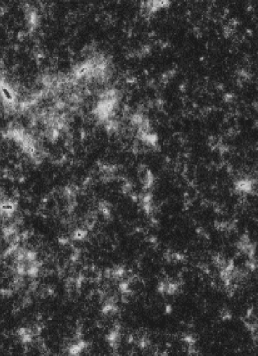
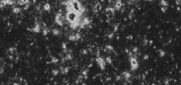
Figure 5: The magnification pattern on a 1^∘ field for an Einstein-de Sitter (upper panel) and open (lower panel) model with $\Omega_{\rm m}=0.3$. The typical value of the magnification in these fields is $5\%$.

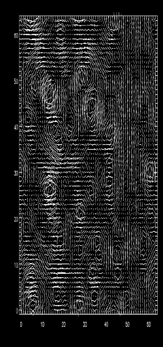
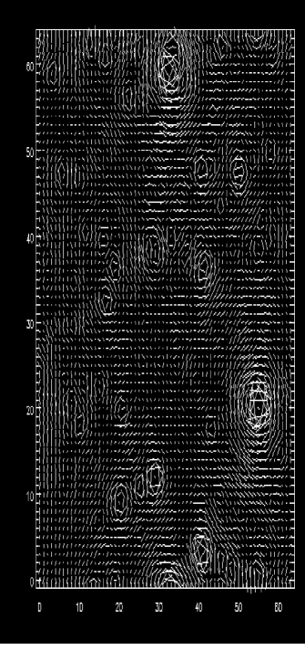
Figure 6: The shear pattern on a 1^∘ field for Einstein-de Sitter (upper panel) and open (lower panel) models, corresponding to the magnification patterns of figure 5. The open model produces a shear pattern dominated more strongly by clusters and groups of galaxies.

As a first check on the accuracy of our results, the power spectra of the convergence $\kappa$, the shear $\gamma$, and of the antisymmetric part of $\Phi$ are shown for the SCDM model in figure 7. We have used the SCDM model as it has more power on small scales and therefore stronger nonlinear effects than the other models. In the weak lensing approximation the power spectra of the first $\kappa$ and $\gamma$ should be the same – this is verified by the measured spectra in figure 7, which are nearly identical except at very small $l$. The power spectrum of the anti-symmetric part of the Jacobian, $(\Phi_{12}-\Phi_{21})$, on the other hand is smaller by more than 3 orders of magnitude. These results imply that $\Phi$ can be well approximated as a symmetric matrix obtained from the 2nd derivatives of a scalar potential. This explicitly shows that the corrections produced by quadratic terms, such as the one which produces image rotation, are samll. This numerically verifies one of the assumptions of weak lensing.

Figure 7: The power spectra of the convergence $\kappa$, shear $\gamma$ and the anti-symmetric part of the Jacobian matrix $\Phi_{12}-\Phi_{21}$ are shown by the solid, dashed and dotted curves respectively. The power spectra of $\kappa$ and $\gamma$ are analytically predicted to be identical. The power spectrum of $\Phi_{12}-\Phi_{21}$ is the same as the power spectrum of the rotational component. This is at least 3 orders of magnitude smaller than that of $\kappa$, thus validating one aspect of the weak lensing approximation. The model used is SCDM, for which nonlinear effects are strongest.

Figure 8: The convergence power spectrum for different models. For the cosmological model indicated by $\Omega_{\rm m}$ and $\Gamma$ in the panel, the power spectrum from ray tracing is compared with the linear (long-dashed) and nonlinear analytical (short-dashed) predictions. The power spectra are averaged over 5-10 ray tracing realizations; the error bars show the 1-$\sigma$ deviation about the mean. The angular size of the field is 2.8^∘ for the $\Omega_{\rm m}=1$ models, 3.9^∘ for the open model, and 3.5^∘ for the $\Lambda-$model. The upper x-axis labels in the upper panels give the angle in arcminutes corresponding to $\pi/l$.

The convergence power spectrum for the 4 CDM models is compared to analytical predictions in figure 8. The error bars show the 1-$\sigma$ dispersion about the mean obtained from 5-10 realizations of the ray tracing. The dashed curves show analytical predictions based on the linear and nonlinear power spectrum respectively. Details of the nonlinear calculation are given in Jain & Seljak (1997). The x-axis shows the wavenumber in inverse radians. The upper panels also show the corresponding angle given by $\pi/l$, expressed in arcminutes. The most striking aspect of figure 8 is that the power spectrum is almost entirely in the nonlinear regime. The measured power is significantly enhanced over the linear spectrum on all scales probed by fields of order 3-4^∘ on a side; for $l\sim 10^{4}$ the enhancement is more than an order of magnitude. Thus with data from upcoming weak lensing surveys we expect to probe primarily the nonlinear regime of gravitational clustering.

The agreement of the spectrum measured by ray tracing with the analytical predictions of Jain & Seljak (1997) is very good. There are slight differences in shape for some of the models but these are not much larger than the expected accuracy of the analytical predictions (Jain, Mo & White 1995; Peacock & Dodds 1996). Indeed, the 3-dimensional density power spectra of the same set of simulations show the same level of discrepancy between the N-body and the analytical predictions, especially for the open model (Jenkins et al. 1997). Thus the fitting formulae are not sufficiently accurate for all models on the smallest scales. The discrepancy at high-$l$ is in part due to limited small-scale resolution as discussed in the previous section. The numerical suppression is caused by the finite grid spacing, and the smoothing of the projected density on low-redshift planes (necessary to suppress the white noise contribution from small particle number). This reduces the power for $l$ smaller than 1/2 the Nyquist frequency $\sim 10^{5}$ radians^-1, which should set the resolution scale from grid effects. Aside from the slight discrepancies in the shape of the power spectra and at high-$l$, the agreement with analytical predictions provides a powerful check on the validity of the weak lensing assumptions made in the analytical calculation as well as an estimate of the dynamic range of the ray tracing results.

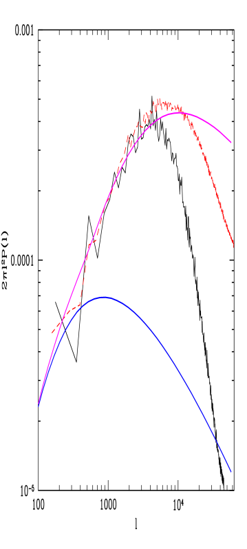
Figure 9: Comparison of the convergence power spectrum from ray tracing through PM and P³M simulations. The solid line is for the PM spectrum and the dashed line for the P³M spectrum.

Figure 9 shows a comparison of the convergence power spectrum from PM and P³M simulations with the analytical predictions. Such a comparison is useful for assessing the resolution provided by the PM simulations. The simulated spectra agree with the analytical predictions over two decades in wavenumber. The PM spectra suffer from numerical smoothing on scales about 4 times as large as the P³M. This shows that for power spectrum measurements PM simulations suffice for $l<5000$. This does not mean that the PM simulations are accurate for higher order statistics on the same scales: these comparisons are shown in the following sections.

4.1 Effects of sample size and noise

Figure 10: The convergence power spectrum corrected for the mean value in a given realization. The non-zero mean value of $\kappa$ within a field $0.4^{\circ}$ on a side is used to correct the computed power spectrum. The correction is made by adjusting the measured $\kappa$ for the change in the growth factor required to produce the finite mean value (see text for details). The power spectra shown in all four panels are for the $\Omega_{\rm m}=0.3$ open CDM model. The upper left panel shows the uncorrected spectrum, obtained by averaging 64 realizations. The lower left panel shows the corrected spectrum for which the error bars are smaller by nearly a factor of 2 at high $l$. The upper right and lower right panels show the power spectra, corrected using wrong values of $\Omega_{\rm m}$, $\Omega_{\rm m}=1$ and $\Omega_{\rm m}=0.15$ respectively. This increases the scatter in the power spectra compared to the correct value of $\Omega_{\rm m}$ and could in principle be used to determine $\Omega_{\rm m}$.

The error bars shown in figure 8 indicate the dispersion in the measured power for fields of size $\sim 3-4^{\circ}$ on a side. On these scales the largest modes are linear and the fluctuations on large scales are due to sample variance, i.e. the small number of modes available to measure the power. For smaller fields even the largest modes are nonlinear and become coupled to the modes on smaller scales. In this case the power spectrum variation is no longer dominated by the finite number of modes, rather it is determined by the strength of mode coupling which depends on the power on scales of the survey. The error bars in the upper left panel of figure 10 can be compared with those in figure 8 to see the effect of reducing the field size.

Figure 11: The convergence power spectrum with noise due to the intrinsic ellipticities of source galaxies. The power spectrum is computed including the intrinsic ellipticity dispersion on fields with side-lengths $3.9^{\circ}$ for the $\Omega_{\rm m}=0.3$ open CDM model. The error bars are computed by averaging over 10 realizations.

Figure 12: The smoothed rms value of $\kappa$ and $\gamma$ versus angle $\theta$. The analytical predictions are given by the dashed curves as in the previous figure. The circles and triangles give the ray tracing results for one realization, while the solid line gives the average over four different realizations. There are negligible differences between realizations in the rms. On large scales, for diameter $2\,\theta\lower 2.15277pt\hbox{$\;\buildrel>\over{\sim}\;$}L/10$, where $L\sim 3-4^{\circ}$ is the side-length of the field, the rms measured from ray tracing is suppressed due to the finite size of the field.

In figure 10 we explore a way of reducing the scatter in the measured power on a set of fields of $0.4^{\circ}$ on a side. The main source of scatter with small field sizes arises from the fact that in a given redshift bin, the mass density deflecting the light rays is not equal to the global mean at that redshift. The effect of the departure from the global mean density can be approximated by changing the growth factor for the density perturbations within that region, i.e. using the growth factor for a different value of $\Omega_{\rm m}$. This is another way of describing the dominant effect of nonlinear mode coupling. The mean $\kappa$ measured on the source plane is a weighted integral of the density over redshift. It therefore provides a measure of the change in the density growth factor averaged over redshift with a known window function. We could use the value of the measured mean $\kappa$ in that region (which could be obtained, for example, from a larger sample, or from the number counts) to “correct” the measured power spectrum of $\kappa$ for the fluctuations in the mean density along the line of sight. To implement this procedure with observational data would require assuming a value of $\Omega_{\rm m}$; one could repeat the procedure with varying $\Omega_{\rm m}$ until the error bars are minimized. In principle this offers a method of measuring $\Omega_{\rm m}$ from the fluctuations in the mean $\kappa$ in different fields, but is likely to give a poorer constraint than using higher moments of the distribution. Nevertheless, the fact that for the correct value of $\Omega_{\rm m}$ the fluctuations are reduced by nearly a factor of 2 implies that the main source of error in the power spectrum are the fluctuations on scales larger than the beam, which in this case are of order unity. This source of error dominates the effect of finite number of modes, especially on scales much smaller than the field size for which there are many modes per wavenumber bin.

So far we have discussed the effects of sample variance that would be present even if the data had no noise and the galaxies were intrinsically circular. The dominant source of noise in observational data are the intrinsic ellipticities of galaxies. Figure 11 shows the power spectrum measured from simulated data with $2\times 10^{5}$ galaxies per square degree whose intrinsic ellipticities are Gaussian distributed with an rms of 0.4 for each component. Clearly at high $l$ the ellipticity noise dominates and prevents the determination of the true power spectrum for $l\lower 2.15277pt\hbox{$\;\buildrel>\over{\sim}\;$}10^{4}$. For $300\lower 2.15277pt\hbox{$\;\buildrel<\over{\sim}\;$}l\lower 2.15277pt\hbox{$\;\buildrel<\over{\sim}\;$}3000$, the power spectrum can be measured with an accuracy of a few tens of percent from of order 10 fields, each a degree on a side. This wavenumber range corresponds to length scales of $1-10\,h^{-1}$Mpc at redshifts of 0.3-0.5 that dominate the lensing contribution. Thus the mass power spectrum can be estimated most accurately over this range of scales. To reach length scales approaching $100\,h^{-1}$Mpc sparse sampling with sufficient number of degree sized fields is required (Kaiser 1998). We emphasise that these conclusions have not taken into account observational noise such as seeing that may degrade the signal, as discussed in Section 1. We have compared our estimates of the sample size with the linear estimates of Blandford et al. (1991), Kaiser (1992, 1998), Jain & Seljak (1997) and Hu & Tegmark (1999). We find that the error bars of figure 11 fluctuate about the linear estimates for $l<3000$, while they are dominated by shot noise for higher $l$. The estimation of cosmic variance bears further examination with simulations that do not need to use the same box multiple times, as this may be affected by corrrelated structures.

For some data sets it may only be feasible to measure moments in real space rather than Fourier space. The rms of $\gamma$ and $\kappa$, smoothed with a top-hat window in real space, is shown in figure 12. The two rms values on different smoothing angles agree very well as expected analytically. The values also agree well with the nonlinear analytical predictions. The slight discrepancies at small scales are consistent with the discrepancies in the power spectra for the same models. On large scales the rms falls below the analytical values due to the missing power from long wave modes. The difference is larger than for the power spectrum because the rms at a given angle involves an integral over all wavenumbers. The fluctuations between different realizations are much smaller for the rms than for the power spectrum, again because it is an integral over a broad range of wavenumbers.

5 Measures of non-Gaussianity

Given a patch of the sky with measured ellipticities of background galaxies we would like to extract cosmological information with as little loss as possible. For a Gaussian distribution (likely to be valid on large scales for popular models of structure formation) one only needs to extract the power spectrum from the data, which completely determines all the statistical properties of weak lensing. There is a well defined procedure for doing this (Seljak (1998)), based on a maximum likelihood (ML) method: one writes the full probability distribution (likelihood function) for the measurements as a multivariate Gaussian, whose unknown parameters are the power spectrum coefficients as a function of scale. By finding the maximum of the likelihood function we find the estimated values of the power spectrum coefficients. The method is asymptotically unbiased and minimum variance. One can also derive a quadratic estimator from this ML method, which is easier to compute and leads to the same ML solution (Seljak (1998)). For scales small compared to the survey size the quadratic estimator reduces to a simple Fourier method (Kaiser 1998): the Fourier transform coefficients of the reconstructed $\kappa$ are squared and added together for all the modes contributing to a given power spectrum bin. The power spectrum estimates are finally obtained by subtracting the noise contribution.

For non-Gaussian distributions, which arise due to nonlinear gravitational evolution on small scales, the problem of how to optimally extract the information in the data is more difficult to solve. Nonlinear evolution develops correlations between Fourier modes which were uncorrelated in the linear regime. This mode-mode coupling does not show up in the two point correlator of Fourier modes because of translational invariance, but is present in all the higher moments. The full likelihood function would have to describe all these correlations and is therefore not amenable to analytic expressions.

Given that the full likelihood function is not achievable, what is the next best thing to do? In previous studies on nonlinear clustering various statistical descriptions of non-Gaussianity have been developed. Among these are moments, N-point correlation functions, the bispectrum, Edgeworth expansion of the pdf etc. In light of the many possible statistics one can devise, it is difficult to take a rigorous, systematic approach. Nevertheless, the fact that the non-Gaussian signatures have been produced by gravity allows one to make some general statements regarding the merits of different estimators. We should emphasize that we are interested in the best possible statistic to determine $\Omega_{\rm m}$, the principal free parameter in addition to the power spectrum that weak lensing can probe. In some applications of non-Gaussianity, such as in galaxy clustering, one is interested both in the biasing relation and $\Omega_{\rm m}$. To break the degeneracy between the two the data have to be compressed in more than a single number (e.g. bispectrum, cumulant correlators or three-point correlation function; Scoccimarro et al. 1998, Szapudi 1998). These complications are not present in the case of weak lensing, so we can concentrate on the simplest statistics and compress all the information on $\Omega_{\rm m}$ into a single number.

The first question is whether one should look for non-Gaussian signatures in Fourier space or in real space. We may for example compare the third moment in real space $\langle\kappa(\hbox{\boldmath{$r$}})^{3}\rangle$ (or skewness $S_{3}=\langle\kappa(\hbox{\boldmath{$r$}})^{3}\rangle/\langle\kappa(\hbox{\boldmath{$r$}})^{2}\rangle^{2}$, where the insertion of the extra powers of second moment makes $S_{3}$ independent of power spectrum amplitude in perturbation theory) to the bispectrum, defined in Fourier space as $\langle{\tilde{\kappa}}(\hbox{\boldmath{$l$}}_{1}){\tilde{\kappa}}(\hbox{\boldmath{$l$}}_{2}){\tilde{\kappa}}(\hbox{\boldmath{$l$}}_{3})\rangle$ with $\hbox{\boldmath{$l$}}_{1}+\hbox{\boldmath{$l$}}_{2}+\hbox{\boldmath{$l$}}_{3}=0$. We found the bispectrum to be a very noisy statistic, so that even with a large number of realizations the signal remained very weak. In contrast, the skewness shows a clear signature of nonlinear evolution and can be measured robustly, as shown in the next section. This is not surprising, since the bispectrum has one more parameter (the shape of the triangle of Fourier modes) and one has to compress the data from different triangle shapes first to obtain more robust information. The question of how to combine this information is however not trivial. The skewness in real space is one way to compress this information into a single number at a given scale, and while it may not be optimal it has the advantage of being physical and easy to compute. Note that to observe it we need to reconstruct convergence from the shear, which is only feasible with sufficiently large fields. As we show below large fields are required anyways for the signal to be observable, so this is less of a constraint than it would appear at first. All the results we show are based on convergence as reconstructed from shear and include any additional systematic effects that could in principle arise from this procedure. One example of such effects is forcing periodic boundary conditions to the data. This generates unphysical structure on the edges of the field, but the effects are very small and do not show up as a significant effect in any of the statistical tests we applied.

The other reason for using real space methods is that the action of gravity is quite localized in real space: it approximately preserves the relative rankings of density peaks, but enhances their contrast in the distribution because of nonlinear evolution. This is the reasoning behind the Gaussianization procedure (Weinberg (1992)), which attempts to reconstruct the primordial density field by mapping the density pdf into a Gaussian. Should this mapping work perfectly, we would have the full distribution function for the data, which would be written as a multivariate Gaussian on a nonlinear transformation of the density field (exactly the transformation that brings the pdf into a Gaussian form). As discussed below, we found that this mapping does not work sufficiently well in practice to reconstruct the linear distribution.

Before we proceed, we need to address the issue of how to combine information obtained from different scales. For Gaussian theories information from different scales can be combined for higher statistical significance of the result. This can be done because in the linear regime modes are independent, allowing information from different scales to be combined. Once the second moments (or power spectrum) are determined there is only one additional parameter that we aim to determine from weak lensing data, the density parameter $\Omega_{\rm m}$ (ignoring the differences between open and cosmological constant models with the same $\Omega_{\rm m}$). This parameter can be determined from a range of scales. The information from different scales however cannot be combined independently. If nonlinear evolution were to only enhance the contrast, but not change the initial ranking order of density values (as assumed in Gaussianization), then one could argue that the smallest scale includes all of the information present in the largest scales as well.

We have tested this by mapping the pdf into a Gaussian on a small scale (Gaussianize the data) and then constructing the pdf on a larger smoothing scale. We found that the pdf on the larger scale was very close to a Gaussian, so that most of the information on the non-Gaussianity of the pdf was used up by the mapping on the smaller scale. However, there are still mode-mode correlations present in the transformed data, so Gaussianization as a way to obtain their full likelihood function does not work sufficiently well. These correlations are not accessible by using the pdf in real space; it would require a much more complicated method to add this information to the one from pdf.

In the absence of noise, the smallest scales are the most sensitive to nonlinear effects. Noise masks information more on small scales, so there exists an optimal scale where noise is still not dominant and non-Gaussian effects are large enough to look for the non-Gaussian signal. The question of how this optimal scale can be determined is addressed below. The error on the estimate of $\Omega_{\rm m}$ is then given by the scatter at this optimal smoothing scale. Combining the data from different smoothing scales does not improve the accuracy on $\Omega_{\rm m}$, but is still useful as a consistency check.

6 Results on non-Gaussianity

6.1 The one point distribution function (pdf)

We now turn to the use of non-Gaussian signatures induced by lensing to measure cosmological parameters. In this section we will discuss the one point distribution function (pdf). The pdf has been previously studied by Wambsganss et al. (1995, 1998) who focussed on the high magnification regime. We will first present pdf’s for various cosmological models in the absence of noise, highlighting qualitative differences between them. Simulated data with noise due to the finite number density of galaxies with large intrinsic ellipticities will then be used to address the question of how to extract $\Omega_{\rm m}$ from weak lensing data.

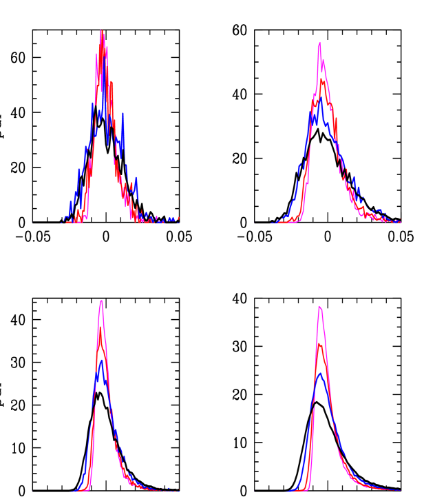
Figure 13: Pdf of $\kappa$ at four smoothing scales, 8’ (upper left), 4’ (upper right), 2’ (lower left) and 1’ (lower right). From top to bottom at the peak values (thin to thick lines) are the open model, cosmological constant model, flat model (all with $\Gamma=0.21$) and the standard CDM model (with $\Gamma=0.5$).

The qualitative features of the pdf are illustrated in figure 1 and figure 13. Figure 13 shows the pdf for four different cosmological models at four different smoothing lengths, assuming the sources are at $z=1$. The models are: open $\Omega_{\rm m}=0.3$ model, flat $\Omega_{\rm m}=0.3$ model, flat $\Omega_{\rm m}=1.0$ model (all with the shape $\Gamma=\Omega_{\rm m}h=0.21$) and flat $\Omega_{\rm m}=1.0$ with $\Gamma=0.5$ (standard CDM), from top to bottom at the peak values of the pdf. These are the same models as in figure 8 for the power spectrum. At the largest smoothing length (8’ top hat radius, upper left) the pdf’s are close to a Gaussian. There is a large scatter because of the small number of cells at this smoothing level (about 100 per simulation averaged over 10 realizations in this case). We use the same smoothing length for all the models which will facilitate comparison of the pdf’s with noise added. Since the models are normalized to satisfy cluster abundance constraints the rms values at a given scale are comparable (Jain & Seljak (1997)), so that if the pdf’s for different models were Gaussian, the curves would be very close together.

As we decrease the smoothing lengths shown in figure 13 to 4’ (upper right), 2’ (lower left) and 1’ (lower right), the pdf becomes more and more non-Gaussian. This leads to two qualitatively different features. Overdense regions have collapsed into dense structures giving rise to a tail of high $\kappa$ that extends to larger and larger values as we reduce the smoothing. At the smallest scales $\kappa$ approaches unity in some regions where strong lensing can occur. In the quasilinear regime on larger scales the amount of non-Gaussianity depends on the rms in the density perturbations at the smoothing scale. We may loosely describe the smoothing scale in 3-d as the angular smoothing scale in 2-d multiplied with the half distance to the galaxies, where the lensing probability peaks. Comparing between an open and flat model with the same rms $\kappa$ one sees that a larger rms $\delta$ is needed in the open model, to compensate for the weaker focussing effect due to the smaller density $\rho$. A larger rms $\delta$ implies non-Gaussian signatures are more important and lead to an enhancement of the pdf at large positive $\kappa$. This high density tail is also the essence of the moments method to determine $\Omega_{\rm m}$ (next section; see also Bernardeau et al. (1996); Jain & Seljak (1997)). Note that the pdf’s for open and flat low density models are visually quite similar. This is quantified in more detail below.

For negative $\kappa$ there is an even more robust qualitative difference. Nonlinear evolution sweeps matter from underdense regions and puts it into collapsed halos or filaments and sheets connecting them. This happens very early in an open universe, so that there are large regions of empty space throughout the line of sight. Many lines of sight propagate through empty space in such a model and the pdf peaks sharply very close to the smallest possible value at small smoothing lengths and drops to 0 rapidly below that. In a flat universe clustering evolves more rapidly at low redshift, so that the universe is more weakly clustered at $z\lower 2.15277pt\hbox{$\;\buildrel<\over{\sim}\;$}1$ compared to an open universe. In addition, cluster abundance normalization gives a lower amplitude for fluctuations in a flat universe at the 10 $h^{-1}$Mpc scale even at the present epoch. For a flat universe the peak in the pdf is thus not close to the minimum value and its shape is less steep, at least for smoothing scales of 1’ and larger.

Figure 14: Pdf of $\gamma$ smoothed on a scale of 2’. The upper two panels show the pdf and cumulative pdf of the open (dashed) and flat (solid) models with $\Gamma=0.21$ spectra. The lower left panel shows the difference of the pdf from a Gaussian with the same rms. The lower right panel shows the ratio with the same Gaussian for the two models.

The minimum value of reconstructed $\kappa$ is proportional to the density parameter $\Omega_{\rm m}$. This is the reason that the minimum value of $\kappa$ in an open universe is much smaller than the corresponding value in a flat universe at small smoothing angles, even if the rms is comparable or even larger. The minimum value of $\kappa$ can be used as a direct measure of the density in the universe, once the redshift distribution of background galaxies is known. This does depend somewhat on the geometry, as the pathlength and angular scale differ between open and cosmological constant models with the same $\Omega_{\rm m}$. The empty beam gives the minimum value of $\kappa=-0.12$ for $\Omega_{\rm m}=1$ compared to $-0.04$ for the open $\Omega_{\rm m}=0.3$ model and $-0.06$ for the cosmological constant model. Note however that while in the open universe the measured minimum value is close to the above value (because there are many beams which are almost empty), in the flat universe the lowest measured value is far from the empty beam value. The difference in $\kappa_{{\rm min}}$ is therefore smaller and one has to use the full shape of the pdf in addition to the minimum value to estimate $\Omega_{\rm m}$.

For completeness we show the pdf of $\gamma$ in figure 14. This pdf is harder to interpret than that of $\kappa$, but is simpler to construct from observational data, since it does not require large enough fields to reconstruct $\kappa$ accurately. It is evident that even directly with data on $\gamma$ the pdf can discriminate between models with different values of $\Omega_{\rm m}$. A complete study of the best way to extract $\Omega_{\rm m}$ from the pdf of $\gamma$ constructed from noisy data will not be presented here. We proceed instead with a detailed exploration of the non-Gaussian features in the pdf of the reconstructed $\kappa$.

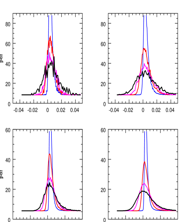
Figure 15: Pdf’s for the open $\Omega_{\rm m}=0.3$ model for sources at four redshifts: from top to bottom at the peak values (thin to thick lines) $z=0.5$, $z=1$, $z=2$ and $z=3$. The smoothing lengths in the different panels are the same as in figure 13.

Figure 13 assumes all the galaxies are at $z=1$. Figure 15 shows how the pdf changes with the redshift of galaxies for the open model. From top to bottom are pdf’s for sources at $z=0.5$, $z=1$, $z=2$ and $z=3$. The deviations from Gaussianity are larger at low $z$. This is because as $z$ increases, one projects a larger number of independent regions. By the central limit theorem this leads to a Gaussian distribution, even though the 3-d pdf of density is very non-Gaussian (approximately a lognormal). On the other hand, the rms of the convergence (the width of the pdf) is increasing with redshift, so that the observability of the effect is likely to increase with redshift, because noise masks the non-Gaussian signal when the rms is small.

6.2 Pdf of $\kappa$ from simulated noisy data

From the considerations above it follows that if one could measure the pdf on small scales directly one could easily determine $\Omega_{\rm m}$. Unfortunately, this is not feasible because of noise. As discussed in the introduction the main source of random noise is the intrinsic ellipticities of background galaxies. In addition, at faint magnitudes measurement errors can cause a significant error in the ellipticity determination. We will model the ellipticity noise as a Gaussian with 0.4 dispersion for each component, roughly in agreement with observational constraints. The Gaussian assumption for the noise is not crucial in this context. The data used is first smoothed, which makes the noise more Gaussian. In addition, even if the noise is non-Gaussian it will not create an asymmetry between positive and negative $\kappa$, so at least for statistics like the odd moments this will not introduce a bias. In practice one should use the actual statistical distribution of ellipticities, which can be obtained from the data itself under the assumption that in the unsmoothed data, ellipticities induced by weak lensing are negligibly small.

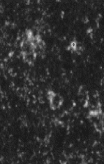
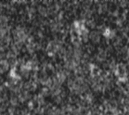
Figure 16: The reconstructed convergence field from ellipticity data on a single 3^∘ field, smoothed on the scale where the noise power spectrum exceeds the signal power spectrum. The right panel shows the reconstructed field using randomly distributed galaxies at $z=1$, with each component of the intrinsic ellipticity randomly drawn from a Gaussian distribution (details are given in the text). The left panel shows the field without noise.

The number density of galaxies depends on the limiting magnitude of the observation. Here we assume $2\times 10^{5}$ galaxies per square degree, which is at the limit of ground based observations with several hour exposures (e.g. Luppino & Kaiser 1997). As before all the galaxies are placed at $z=1$. Our goal is to check using realistic examples if the signal is detectable and what method is best to analyze the data; the details will clearly depend on the specifics of the survey one has in mind. To generate a noisy version of the data we randomly generate galaxy positions on a square grid of a given size and add the weak lensing shear to a random ellipticity component in each of them. We then reconstruct $\kappa$ from these noisy data using the relation between the Fourier transforms of $\kappa$ and $\gamma$, again assuming periodic boundary conditions:

$$\hat{\kappa}(\vec{l})=\frac{l_{1}^{2}-l_{2}^{2}}{l^{2}}\ \hat{\gamma}_{1}(\vec{l})\ +\ \frac{2l_{1}l_{2}}{l^{2}}\ \hat{\gamma}_{2}(\vec{l})\ .$$ (28)

The reconstructed $\kappa$ field smoothed at the scale where noise exceeds the signal is compared to the same field without noise in figure 16.

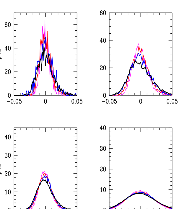
Figure 17: The pdf of $\kappa$ for different smoothing scales and cosmological models, as in figure 1, but with noise added.

Figure 17 shows pdf’s for all the models in figure 13, with noise added. On large scales the noise is negligible and the pdf’s are similar to the no noise case. On very small scales the noise is large and dominates over the cosmological signal, so that the pdf is simply a Gaussian with rms$=0.4/N_{\rm gal}^{1/2}$, where $N_{\rm gal}$ is the mean number of galaxies in a smoothing patch. In both limits the distribution is Gaussian, so we cannot learn anything about non-Gaussianity. In the intermediate regime, on scales of $2^{\prime}$ and $4^{\prime}$, differences between models are still visible. One can hope that there is sufficient signal to noise to extract useful information from the data. We discuss next what the optimal scale is and what statistics are best to extract the signal from the data.

6.3 Moments and other reduced statistics

Having argued that real space statistics exhibit stronger non-Gaussian signatures we need to decide which to choose. The first set of statistics to try are the moments $S_{N}=\langle\kappa(\hbox{\boldmath{$r$}})^{N}\rangle/\langle\kappa(\hbox{\boldmath{$r$}})^{2}\rangle^{N-1}$, for $N=3$ this is the skewness already introduced above. Although one may argue that the pdf contains more information than any of the reduced statistics, the moments can nevertheless be useful because of their simplicity and relative model independence. One advantage of moments is the availability of perturbation theory, with which one can compare the observations on large scales. The main disadvantage is that the moments are sensitive to rare events in the tails of the distribution. The results can be strongly dependent on the presence or absence of a few clusters (Colombi, Bouchet & Schaeffer (1994); Szapudi & Szalay (1996)). This has two consequences: first, sampling variance becomes a more important source of noise as we progress from lower to higher order moments. Second, numerical accuracies of simulation codes become an issue and it becomes difficult to accurately calibrate the observations in the nonlinear regime. This has prompted some workers to try alternatives such as the moments of absolute values (Nusser & Dekel 1993; Juszkiewicz et al. 1995). These are less sensitive to the rare events, but are more sensitive to the presence of noise as shown below.

Based on these arguments we will concentrate on four low order moments, all of which can be expressed in terms of the lowest nonvanishing contribution from the third moment $S_{3}=\langle\kappa^{3}\rangle/\sigma_{\kappa}^{4}$ and so can be compared to perturbation theory predictions. The simplest way to compute $S_{3}$ is simply by its definition above. This statistic is plotted in the lower right panel of figure 18. Shown are simulation results for the same cosmological models as in figure 13, together with the perturbation theory results shown as the dashed lines. The perturbation theory values have been analytically computed using the expressions given in Bernardeau et al. (1997) and Jain & Seljak (1997). The important point is that $S_{3}\propto\Omega_{\rm m}^{-1}F(n)$, where $F(n)$ is a weak function of the shape of the power spectrum, but not of its amplitude. That this function only weakly depends on the spectral shape is seen from the comparison of $\Gamma=0.21$ and $\Gamma=0.5$ models in figure 18, both of which give almost identical perturbation theory results. At a given redshift the perturbation theory predictions depend somewhat on the assumed geometry and pathlength, causing a difference of order 15% between a cosmological constant model and an open model with the same matter density $\Omega_{\rm m}$.

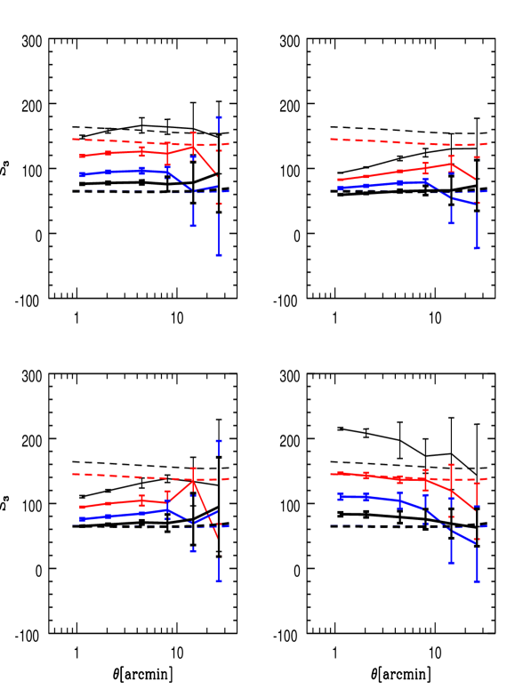
Figure 18: $S_{3}$ statistics from 4 different measures: second moment over positive values (upper left), negative values (upper right), difference between negative and positive values (lower left) and the third moment (lower right). From top to bottom (thin to thick lines) are the open model, cosmological constant model, flat model (all with $\Gamma=0.21$) and the standard CDM model (with $\Gamma=0.5$). Dashed curves are perturbation theory results. Errors are based on the scatter of 5-10 realizations.

The results of N-body simulations agree with perturbation theory on large scales, although the scatter in individual realizations is large even in the absence of noise. On small scales $S_{3}$ rises above its perturbation theory value by different amounts depending on the model. For the open model the rise above the perturbation theory value is a factor of 2 on very small scales, while for the cosmological constant model there is no rise at all. Moreover, there is also a dependence on the shape of the power spectrum, resulting in different predictions for $S_{3}$ between $\Gamma=0.21$ and $\Gamma=0.5$ models. Nevertheless, the difference between the low and high $\Omega_{\rm m}$ models is clearly seen. Thus in the absence of noise due to the finite number of galaxies, the statistical significance would be enormous. The interpretation of the result however is complicated by the shape and geometry dependences on very small scales. For this reason it is better to use the data on more intermediate scales, where the deviations from perturbation theory are smaller. This conclusion will be further strengthened when we discuss the effects of noise.

Two other statistics related to $S_{3}$ in perturbation theory are $\langle\kappa|\kappa|\rangle_{\kappa>0}$ and $\langle\kappa|\kappa|\rangle_{\kappa<0}$. These statistics have been suggested by Nusser & Dekel (1993) and Juszkiewicz et al. (1995) as a way to reduce the sampling variance from rare events which populate the tails of the distribution and strongly affect the higher moments. Because of quadratic weighting one can expect these statistics to be more robust. The contributions from positive and negative $\kappa$ are separated because they probe different physical regions, halos and voids, respectively. We use the Edgeworth expansion of the pdf around the Gaussian to compute the perturbation theory values of these statistics (Juszkiewicz et al. 1995). At lowest order, the Edgeworth expansion is given by

$$p(\kappa)={1\over\sqrt{2\pi}\sigma_{\kappa}}e^{-\kappa^{2}/2\sigma_{\kappa}^{2}}\left[1+{1\over 6}S_{3}\sigma_{\kappa}H_{3}(\kappa/\sigma_{\kappa})\right],$$ (29)

where $H_{3}(x)=x^{3}-3x$ is the 3rd order Hermite polynomial. The statistic introduced above is then

$$\langle\kappa|\kappa|\rangle_{\kappa>0}=\int_{0}^{\infty}p(\kappa)\kappa^{2}d\kappa=\sqrt{2\over 9\pi}S_{3}\sigma_{\kappa}^{3}\ .$$ (30)

For the $\kappa<0$ statistic one obtains the same perturbation theory value. In figure 18 we plot $S_{3}$ obtained using this method separately for positive values (upper left plot) and negative values (upper right). The predictions of perturbation theory again agree with N-body simulations on large scales, albeit with large scatter. On small scales the positive $\kappa$ statistic remains approximately constant, while the negative $\kappa$ statistic drops in value towards 0. This is expected, because $\kappa$ is bounded from below, so the rms over negative values cannot exceed the minimum value, while the full rms in the denominator continues to grow on small scales.

The fourth statistic we measured is $-\langle{\rm sign}(\kappa)\rangle$, which is the sum over all negative $\kappa$ minus the sum over all positive $\kappa$, normalized by the total number of $\kappa$. This statistic is the least sensitive to the tails and should be very robust to the details in high density regions. Again using the Edgeworth expansion we find at lowest order

$$-\langle{\rm sign}(\kappa)\rangle=\int_{-\infty}^{0}p(\kappa)d\kappa-\int_{0}^{\infty}p(\kappa)d\kappa=(18\pi)^{-1/2}S_{3}\sigma_{\kappa}.$$ (31)

The $S_{3}$ measured from this statistic is plotted in the lower left of figure 13. In the absence of noise it shows the same properties as the statistics discussed above. It agrees with perturbation theory on large scales, but with large scatter. On small scales it does not differ significantly from the perturbation theory value and shows remarkably small scatter. However, these appealing properties do not survive once noise is added, as discussed below.

6.4 $S_{3}$ from simulated noisy data

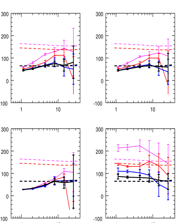
Figure 19: $S_{3}$ statistics, as in the previous figure, but with ellipticity noise added to the simulations.

We now add noise due to the finite number of source galaxies to the simulated maps and compute the same statistics as in figure 18 in a $3^{\circ}\times 3^{\circ}$ field, shown in figure 19. Noise introduces significant scatter and makes some of the statistics biased. The third moment (lower right panel) has the advantage that it is unbiased even in the presence of noise. To show this we can write the measured $\kappa=\kappa_{s}+n$, where $\kappa_{s}$ is the true convergence and $n$ is the noise component. The former has a probability distribution $p(\kappa_{s})$, while the noise we assume to be Gaussian distributed as $p_{n}(n)=(2\pi\sigma_{n}^{2})^{-1/2}\exp(-n^{2}/2\sigma_{n}^{2})$. Then

$$\langle\kappa^{3}\rangle = \int_{-\infty}^{\infty}\int_{-\infty}^{\infty}\kappa^{3}p(\kappa_{s})p_{n}(\kappa-\kappa_{s})d\kappa d\kappa_{s}$$ (32)

$$= \int(\kappa_{s}+n)^{3}p(\kappa_{s})p_{n}(n)d\kappa dn=\langle\kappa_{s}^{3}\rangle,$$

since $\langle\kappa_{s}\rangle=\langle n\rangle=\langle n^{3}\rangle=0$. Note that by symmetry the latter relation still holds even if the ellipticity distribution is not Gaussian. Similarly we can correct $S_{3}$ so that it is unbiased (Hui & Gaztañaga 1998).

In contrast, for the other three statistics noise introduces bias and $S_{3}$ is generally suppressed relative to the case of no noise. This is because in the presence of noise some $\kappa$ switch sign, which reduces the signal from these statistics which are defined relative to the 0 mean. Unlike in the case of $\langle\kappa^{3}\rangle$, one has to correct for noise, which requires knowledge of the full pdf to perform the integrals such as in equation 32. In practice this is best performed with N-body simulations. If one corrects for noise bias one can see from figure 19 that the optimal angular scale for the detection is around $1^{\prime}-5^{\prime}$. The detection is at a several $\sigma$ level for the first method and a similar significance level is achieved if one combines the second and third methods (which use two disjoint parts of the data set), but at the expense of a more complicated noise corrections. The fourth statistic fails completely in the presence of noise, as it gives the same value on small scales for all the models.

To address the question of required survey size, we repeated the above analysis for $2^{\circ}\times 2^{\circ}$ and $1^{\circ}\times 1^{\circ}$ fields. We find that $1^{\circ}\times 1^{\circ}$ field is too small for the signal to be detected at more than a 1-sigma level. The errors are significantly reduced for a $2^{\circ}\times 2^{\circ}$ field, which seems to be the minimum required for a positive detection, at least for the survey depth and density we assumed here. This size is quite realistically achievable in the near future, as there are several multi-square degree surveys under development which will reach the size and depth needed to measure this signal.

To summarize, both the third moment and the combination of the second moments over positive and negative values show clear signature of a non-Gaussian signal even in the presence of noise. The third moment $\langle\kappa^{3}\rangle$ is the most sensitive and is unbiased in the presence of noise bias. On the other hand, it is somewhat more sensitive to numerical calibration errors than the two quadratic weighting methods. It is recommended that all the methods are applied to the data and the results tested for consistency. Moments of order higher than 3 are to be avoided because of sensitivity to the rare events in the tails and to uncertainties in the numerical simulations. The lowest order method, based on the difference between negative and positive values, fails in the presence of noise.

6.5 Comparison of results from PM and P³M simulations

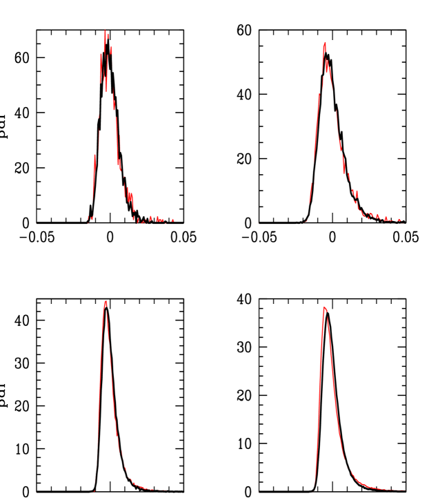
Figure 20: Comparison between the pdf from P³M (thin curves) and PM (thick curves) simulations for the same smoothing angles as in the previous two figures. The model shown is $\Omega_{\rm m}=0.3$, $\Omega_{\lambda}=0$, $\Gamma=0.21$ and $\sigma_{8}=0.85$.

All the results shown above have used P³M simulations. It is instructive to compare them to faster PM simulations, which are expected to agree with P³M simulations except in very dense regions. This is more important on small scales and/or higher moments. Figure 20 shows the comparison between the pdf for PM and P³M simulations for the $\Omega_{\rm m}=0.3$ model. While the P³M simulation has $256^{3}$ particles and is one of the highest resolution simulations existing at present, the PM simulation used $128^{3}$ particles on a $256^{3}$ grid and only required of order 10 CPU hours on a single processor workstation. Nevertheless, the agreement in the pdf is quite good for all the smoothing lengths and only on the smallest scales does one see small differences. These results are reassuring and indicate that if one is using the pdf away from the tails the faster PM simulations suffice. However, the signatures in the tails are more discriminatory, so it is important to test any statistic one is using for its sensitivity to numerical inaccuracies.

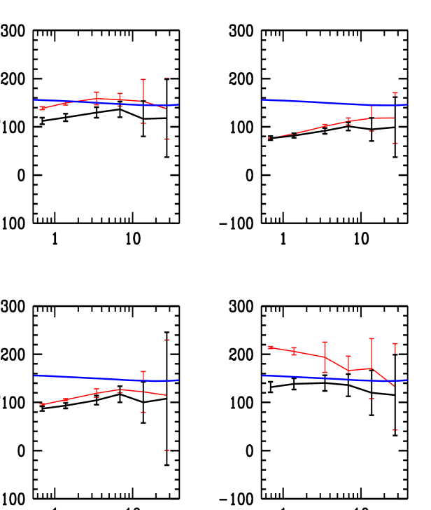
Figure 21: Comparison between P³M (thin upper curves) and PM (thick lower curves) for the same statistics as in figure 18. The model shown is $\Omega_{\rm m}=0.3$, $\Omega_{\lambda}=0$, $\Gamma=0.21$ and $\sigma_{8}=0.85$.

The comparison of results for $S_{3}$ between PM and P³M simulations is shown in figure 21 for the $\Omega_{\rm m}=0.3$ model. On large scales both simulations give results that are in agreement with each other and with perturbation theory. On small scales differences are evident, more significantly for those measures that weight the positive tail of the pdf more strongly. This is especially true for the third moment method (lower right), which is based on averaging $\kappa^{3}$ and so most strongly weights the high density regions. The difference between PM and P³M in this case reaches a factor of 2 on small scales. The PM simulation is clearly inadequate for this statistic. In general these results show that for higher moments the PM simulations have to tested and calibrated with P³M as the resolution range is difficult to estimate a priori. One may worry that the P³M results may also be sensitive to numerical resolution on the smallest scales, so it is better to use statistics most sensitive to the tails on larger scales where the differences are smaller.

7 Likelihood analysis of the pdf

The alternative to moments for probing non-Gaussianity is to use the pdf of the reconstructed convergence. The pdf by definition describes the full distribution of $\kappa$ and so is not unduly sensitive to the high density tails. The simplest way to analyze the pdf is to use the Edgeworth expansion (Juszkiewicz et al. 1995; Kim & Strauss 1998), which expands the pdf around a Gaussian in a Hermite polynomial series. At lowest order one can fit for two free parameters, the variance and skewness (equation 29). To obtain the probability distribution for the measured $\kappa$ we convolve $p(\kappa)$ with the noise probability distribution $p_{n}(n)=(2\pi\sigma_{n}^{2})^{-1/2}\exp(-n^{2}/2\sigma_{n}^{2})$. The convolution integral can be analytically calculated, giving the pdf for the measured $\kappa$

$$p(\kappa|S_{3},\sigma_{\kappa})=\int_{-\infty}^{\infty}p(\kappa_{s})p_{n}(\kappa-\kappa_{s})d\kappa_{s}=$$

$${1\over\sqrt{2\pi(\sigma_{\kappa}^{2}+\sigma_{n}^{2})}}\exp\left[{-\kappa^{2}\over 2(\sigma_{\kappa}^{2}+\sigma_{n}^{2})}\right]$$

$$\left[1+{1\over 6}S_{3}\sigma_{\kappa}\left(H_{3}[\kappa/\sigma_{\kappa}(1+\alpha^{2})]+3{\kappa\over\sigma_{\kappa}(\alpha+\alpha^{-1})^{2}}\right)\right],$$ (33)

where $\alpha=\sigma_{n}/\sigma_{\kappa}$. In the limit $\alpha\rightarrow 0$ noise is negligible and the equation above reduces to the Edgeworth expansion as in equation 29. In the limit $\alpha\rightarrow\infty$ it reduces to a Gaussian with $\sigma_{n}$ rms, in which case the non-Gaussian signature is swamped out by the noise.

To compute the likelihood function on the data we divide the observed region into nonoverlapping square cells and use the average value of $\kappa$ in each cell as the input. The full likelihood function can be written as a product of likelihood functions for individual measurements $\kappa_{i}$,

$$L=\Pi_{i}\ p(\kappa_{i}|S_{3},\sigma_{\kappa}).$$ (34)

Individual $\kappa_{i}$ are not independent (because of correlations in the signal part of convergence; note that noise is uncorrelated for reconstructed $\kappa$ provided that one uses non-overlapping cells for analysis and the number of galaxies in each cell is the same. The later is not exactly true because the galaxies are Poisson distributed, so there are some residual noise correlations left, which decrease as the cell size is increased), so this is not the true multivariate likelihood function for the data even if $p(\kappa_{i}|S_{3},\sigma_{\kappa})$ were the correct pdf. Nevertheless we can continue to use it, as long as we determine the error estimates and possible biases with Monte Carlo realizations of N-body simulations. Given that this is not the true likelihood function we have no reason to expect it to be an optimal estimator, even in the limit of large number of independent measurements. One should really view it as another statistic whose performance should be judged empirically by the scatter in the Monte Carlo realizations. Since it uses information on the full pdf and not just its tails, one hopes that it is a more powerful estimator than the moments.

Figure 22 (upper panel) shows the results of the ML method on the Edgeworth expansion for $S_{3}$ for various models and smoothing scales. The method works well for the flat models, which have a lower $S_{3}$. It agrees with perturbation theory and has very small error bars even on small angular scales where noise is dominant. Visually, the agreement between the Edgeworth expansion and true noise convolved pdf is also quite good. However, in low $\Omega_{\rm m}$ models there is a severe bias on intermediate scales, where the information content is the highest from the moments analysis. The problem is that the Edgeworth expansion of the pdf does not satisfy the positivity condition for a probability distribution. It shows nonphysical oscillations because of the oscillatory nature of Hermite polynomials. For some values of $\kappa$ the pdf is not positive for large $S_{3}$, because the oscillations drive it below 0. This happens only over small regions, but if a measurement falls into one of these regions then $\ln(p)$ around it can have very large negative values and the ML method will drive the estimate for $S_{3}$ and $\sigma$ away from this region into the region where the pdf is positive definite, even if visually the overall fit is much worse. Noise makes the distribution more positive by smoothing out the nonphysical oscillations (Kim & Strauss 1998), but in the present case, with realistic levels of noise due to the finite number of galaxies, weak lensing data appear to be “too good” for a blind application of ML on the Edgeworth expansion. This situation is somewhat paradoxical, because when the data are too good the method fails and one is forced to resort to less accurate methods such as moments. The two ways to remedy this problem are: change the pdf to make it positive definite, or change the analysis method to allow negative pdf. We discuss both of these next.

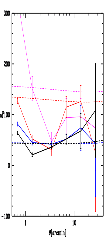
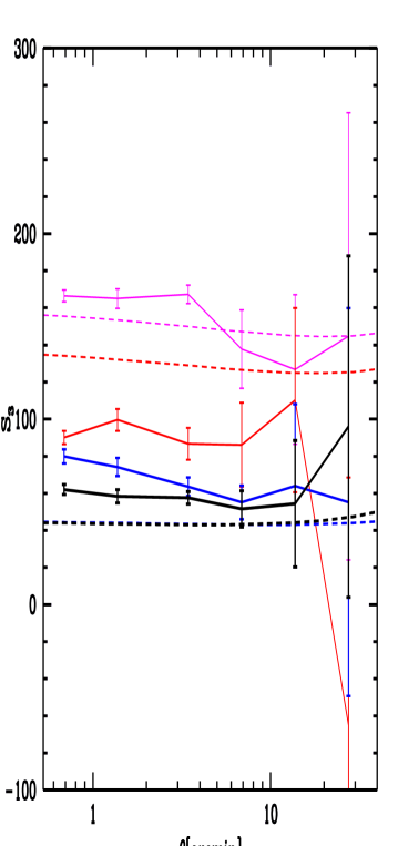
Figure 22: $S_{3}$ using ML (top) and $\chi^{2}$ (bottom) for the same models as in figure 18. Noise has been added to the data.

7.1 Likelihood analysis by fitting to simulations

The failure of the ML method based on the Edgeworth expansion is caused by an unphysical expansion of the pdf. This suggests that it is better to use directly the pdf from N-body simulations, which provide more physical templates against which one can fit the observed data. By spanning a large parameter space of cosmological models one can search for the best model using the ML method. This seems an ambitious program, since it requires obtaining pdf’s from N-body simulations of a dense grid of cosmological models. In practice it is not so formidable, because a given simulation can be used for many different models and because one can use PM simulations, which are fast to compute and are sufficiently accurate away from the tails.

To obtain a set of templates we first ran a number of PM simulations for different cosmological models. For each simulation we chose the shape of the power spectrum (determined by $\Gamma=\Omega_{\rm m}h$ parameter in this case), final $\Omega_{\rm m}$ and final amplitude $\sigma_{8}$. A single simulation can be used not just for the chosen model, but also for models with smaller $\sigma_{8}$. For example, in an $\Omega_{\rm m}=1$ model using an output at redshift $z$ as the output today corresponds to a model with $\sigma_{8}^{\rm new}=\sigma_{8}^{\rm old}/(1+z)$. The shape of the power spectrum remains unchanged and for this case $\Omega_{\rm m}=1$ for all the models. For the case with curvature or cosmological constant earlier time output corresponds to a higher $\Omega_{\rm m}$. Because the shape parameter $\Gamma=\Omega_{\rm m}h$ is unchanged $h$ must then be decreased relative to the original model. Thus a one-dimensional family of models can be spanned by the simulation.

Another transformation that varies the model is a rescaling of the box size. For example, using a 100$h^{-1}$Mpc simulation as a 200$h^{-1}$Mpc simulation changes the shape of the power spectrum so that $\Gamma$ is reduced by a factor of 2. At the same time, for a given output $\sigma_{8}$ is increased, so one has to use an earlier output to obtain the same normalization. It is therefore possible to use a single simulation to describe a two-parameter family of models. Note that the second transformation changes the angular resolution and size of the simulation, so one has to be careful when comparing the results at a given angular scale. Since each PM simulation requires of order 10 CPU hours on a workstation, one can span a dense grid of models in a reasonable amount of time. Here we will present results as a two parameter family ($\Omega_{\rm m}$ and $\sigma_{8}$), although the third parameter $\Gamma$ can easily be added if desired.

We again use the ML method to determine the best model using

$$L=\Pi_{i}\ p[\kappa_{i}|\Omega_{\rm m},P_{\delta}(k)],$$ (35)

where $p[\kappa_{i}|\Omega_{\rm m},P_{\delta}(k)]$ is the pdf for the model determined with $\Omega_{\rm m}$ and $P_{\delta}(k)$. These pdf’s are obtained from the simulations, by binning them into small bins and counting the number of events in them. If there are $M_{i}$ simulated values of $\kappa$ contributing to the i-th bin then the pdf for that bin is given by $p_{i}=M_{i}/(\sum_{i}M_{i})$. To obtain the log likelihood for a given realization we count the number of $\kappa$ in the i-th bin, $N_{i}$, and compute $\sum_{i}N_{i}\ln(p_{i})$. This expression shows how the weight is distributed in the ML method. Around the peak of the pdf there are many events and so $N_{i}$ is large, but $\ln(p_{i})$ itself has a small negative value. For the tails the number of events is small, but each event has a large weight, because $\ln(p_{i})$ can have very large negative value. This way both the peak and the tail of pdf are significant for the ML estimate.

The main drawback with this approach is that one has to use very large simulations to properly sample the tails of the pdf, so that the bins are appropriately populated. If this is not satisfied then even a single event in the real data falling into a bin that was underpopulated completely dominates the rest of the data. Using ML we are therefore faced with the same problem we had with high order moments, which is that sensitivity to the tails implies large uncertanties because of numerical inaccuracies in simulations. Clearly, using information from the rare events enhances the statistical significance of the test, but also increases the “systematic uncertanties” that arise from the uncertainties in the N-body simulations.

7.2 $\chi^{2}$ fitting for the pdf

An alternative to the ML method is a version of the $\chi^{2}$ statistic. $\chi^{2}$ fitting can be used both on the pdf from the simulations as a template or on the Edgeworth expansion. For example, we may compute the difference between measured and expected number of values in the i-th bin for a given model and add up the squares of these differences. We can then again minimize this statistic as a function of the model and explore the errors on the parameters by Monte Carlo simulations. In addition, depending on how one weights the differences one can make the central regions of the pdf more or less dominant compared to the tails. With the weighting according to the expected number of events, the tails become more important and the method becomes similar to the ML method in how it weights the data. No weighting makes the central region more important. Some intermediate weighting is therefore optimal if one wants to maximize both statistical significance and robustness to the N-body results.

We tried several simple weighting schemes and found that even with uniform weighting applied to the Edgeworth expansion, the $\chi^{2}$ statistic gave smaller error bars than moments (figure 22, lower panel). Moreover, $S_{3}$ was relatively constant as a function of angle and the difference between the open $\Omega_{\rm m}=0.3$ and either of the flat models is enormous at $3^{\prime}$. Both flat models with different power spectra gave very similar predictions. Interestingly, the cosmological constant $\Omega_{\rm m}=0.3$ model is much closer to the flat model than to the open one, so it appears that this test is more sensitive to $\Omega_{\rm m}$ for open than for cosmological constant dominated models. Comparison between PM and P³M simulations gave somewhat discrepant results, similar to those in figure 21, so it appears that this method is also sensitive to simulation resolution. Clearly, high resolution N-body simulations are essential if one is to extract the value of $\Omega_{\rm m}$ with high accuracy.

Finally, we also used the $\chi^{2}$ statistic on the pdf templates from simulations. While this statistic is more accurate than all the statistics previously discussed, the increased accuracy does not appear worth the complexity and effort of simulating models spanning a large range of parameters. For example, it is difficult to distinguish between an $\Omega_{\rm m}=0.2$ and $\Omega_{\rm m}=0.3$ model, in the sense that using the $\chi^{2}$ for one model was often better on the other template (with appropriate change in the normalization). The sensitivity therefore appears not to be significantly increased if one uses the true pdf instead of the Edgeworth expansion. Given the increase in complexity of this method its usefulness may be limited, at least until the data become of sufficient quality to necessitate more accurate pdf’s than provided by the simple first order Edgeworth expansion.

8 Discussion

In this paper we have used ray tracing simulations to study the following aspects of weak lensing by large-scale structure: the numerical requirements for simulating weak lensing on angular scales of observational interest, $1^{\prime}\lower 2.15277pt\hbox{$\;\buildrel<\over{\sim}\;$}\theta\lower 2.15277pt\hbox{$\;\buildrel<\over{\sim}\;$}2^{\circ}$; the validity of various weak lensing approximations and of analytical predictions; computation of low-order statistics for different models and estimates of the accuracy with which they can be measured from given survey sizes; estimate of $\Omega_{\rm m}$ using measures of non-Gaussianity from simulated noisy data. Our conclusions are as follows.

Numerical tests and dynamic range from simulations. We have used FFT’s to compute the shear matrix and photon deflections required for propagating light rays in our simulations. The method has been demonstrated to be efficient and accurate provided care is taken with the choice of numerical parameters. We give analytical estimates of the resolution limit implied by (a) the mass resolution and force softening of the N-body simulation, and (b) grid effects in the ray tracing. These estimates were shown to be reliable and can be used to choose numerical parameters such as the grid size.

Lens planes over a broad range of redshifts were found to contribute to the lensing effect. For a given angular size, lens planes at lower-redshift have smaller spatial extent, of order 10 $h^{-1}$ Mpc for degree size fields. Since the lensing efficiency is a broad function of redshift, non-negligible contributions come from small regions that may contain a single over- or under-density with only a small fraction of the particles in the full N-body simulation. This is a complication in achieving sufficient accuracy from ray tracing simulations. On small scales the white noise contribution to the power spectrum from the finite number of particles is difficult to estimate as it depends on the clustering evolution, and therefore on the cosmological model. Given these limitations, to achieve a dynamic range $\lower 2.15277pt\hbox{$\;\buildrel>\over{\sim}\;$}100$ in angular scale, it is necessary to use high-resolution N-body simulations with $\lower 2.15277pt\hbox{$\;\buildrel>\over{\sim}\;$}10^{7}$ particles, and FFT/ray tracing grids of size $\lower 2.15277pt\hbox{$\;\buildrel>\over{\sim}\;$}1000^{2}$ at each lens plane.

Nonlinear effects and comparison with analytical approximations. The power spectra measured from the ray tracing simulations (see figure 8) show that for fields a few degrees on a side the power spectrum of the shear lies entirely in the nonlinear regime. Part of this nonlinearity arises because of the strongly clustered regions at low redshift that affect statistical measures even on degree scales. On scales of observational interest linear theory or perturbation theory do not provide accurate predictions for 2nd and 3rd moments. The skewness measured from a reasonable number of degree sized fields is significantly enhanced over the perturbation theory prediction. Only for the second moment of the shear and convergence can non-perturbative analytical calculations be made (Jain & Seljak 1997) and are found to agree well with the simulations. It is therefore necessary to use simulations in making theoretical predictions and obtaining error estimates for most weak lensing statistics.

The weak lensing approximation is found to be valid to good accuracy. The nonlinear departures discussed above arise from gravitational clustering of the matter, not from any breakdown of weak lensing approximations. There are occasional strong deflections that contribute to the tails of the probability distribution of shear and convergence. But lensing statistics smoothed on scales larger than $1^{\prime}$ do not receive significant contributions from these rare events. An example of a test of the weak lensing approximation is provided by figure 7. The rotational component of the distortion tensor, which arises when significant multiple deflections occur along the same line of sight, is shown to be very small. It is therefore possible to describe the shear and convergence fields as arising from a projected (2-dimensional) gravitational potential.

Sample size for measuring the power spectrum. The power spectrum of the shear directly probes the dark matter power spectrum at intermediate redshifts. Extensive tests have been used to estimate the dynamic range with which we can measure the power spectrum and the accuracy on different scales. For large fields and on large scales, sample variance (finite number of modes) dominated fluctuations in the measured spectrum between different fields and can be reliably estimated using Gaussian statistics. On small scales this variance increases relative to the Gaussian value because nonlinear evolution generates kurtosis. In addition, power spectrum estimates from neighboring bins become strongly correlated. For a quantitative analysis of the variance in the power spectrum it is essential to use numerical simulations. For small fields (below $1^{\circ}$ on a side) mode-coupling becomes the limiting factor in the variance of power spectrum estimates rather than number of modes. We found that for fields smaller than 1^∘, it is possible to correct the power spectrum for fluctuations in the mean convergence within every field. With the correction it is possible to reduce the error on the power by up to a factor of 2, meaning that the errors are dominated by mode coupling on the scale of the sample rather than number of modes within the sample. Measurements of about 10 fields a degree on a side can provide power spectra accurate to a few tens of percent on $10^{3}\lower 2.15277pt\hbox{$\;\buildrel<\over{\sim}\;$}l\lower 2.15277pt\hbox{$\;\buildrel<\over{\sim}\;$}10^{4}$. This procedure depends on the knowledge of mean convergence in the field and its translation into mean density, which makes it an alternative, albeit less sensitive, test of $\Omega_{m}$ to the ones described in sections 6 and 7.

Non-Gaussianity and $\Omega_{\rm m}$. We addressed the issue of how to extract information on the cosmological matter density $\Omega_{\rm m}$ from non-Gaussian signatures in weak lensing data. In the absence of noise, the pdf of the convergence shows a number of characteristic signatures of nonlinear evolution. In particular, high positive values of the convergence are characteristic of collapsed regions, while low negative values show the presence of voids. The high density features depend both on the density parameter and somewhat on the shape of the power spectrum, though the dependence on the latter is reduced by smoothing the data on arcminute scales. The difference between the mean and the minimum convergence is in principle proportional to $\Omega_{\rm m}$. In our simulations the difference does grow as a function of $\Omega_{\rm m}$, but the effect is reduced somewhat because in high $\Omega_{\rm m}$ models structure is more linear at early times, so that there are virtually no empty beams out to $z=1$.

In the presence of noise the nonlinear signatures are masked and require careful calibration with N-body simulations to extract them. Based on an analysis of several statistics we find that the most promising are: $\chi^{2}$ analysis on the Edgeworth expansion of the pdf, the third moment, and the second moment separately over positive and negative values, in decreasing order of statistical significance. The advantage of these measures is that they are simple, agree with perturbation theory on large scales and can be reasonably well calibrated using N-body simulations on small scales. Methods based on a maximum likelihood fit to the Edgeworth expansion of the pdf improve the accuracy of the determination, but can give biased results. Methods based on maximum likelihood or $\chi^{2}$ fits to the pdf from N-body simulations are the most accurate for a given model, but to span a range of models would require a large number of simulations for a relatively small gain in accuracy.

Noise due to the intrinsic ellipticities of galaxy images masks the signal on very small scales. For the second and third moment the optimal regime is around a few arcminutes, while $\chi^{2}$ on the Edgeworth expansion can give reliable results to significantly smaller scales. With a several degree sized survey of reasonable depth one can determine $\Omega_{\rm m}$ to within about 0.1-0.2 for open models, and somewhat worse for cosmological constant dominated models, based on the statistical errors. The accuracy is also limited by systematic effects, such as the shape and amplitude of the power spectrum. These effects can be modeled with a power spectrum analysis of the same data. Another source of systematics is calibration with N-body simulations. Based on comparisons between PM and P³M simulations we find that the calibration with N-body simulations is relatively secure on a few arcminute scales, while on smaller scales the differences for some of the statistics are quite significant. This is particularly true for the third moment, which is very sensitive to the tails of the distribution. For this reason we did not explore moments higher than the third, such as kurtosis, which would be even more sensitive to the resolution of the simulation. Thus well calibrated, high resolution simulations are essential to probe the high density tails of the pdf. Finally, detecting non-Gaussianity in the weak lensing signal also provides a direct detection of nonlinear evolution of the dark matter. If the results from such an analysis are found to agree with other tests it would provide strong support for the gravitational instability paradigm.

References

- (1) Babul, A. & Lee, M.H. 1991, MNRAS, 250, 407
- (2) Bartelmann, M. & Schneider, P. 1991, A&A, 248,353
- (3) Bartelmann, M., Huss, H., Colberg, J.M., Jenkins, A. & Pearce, F.R. 1998, A&A, 330, 1
- Bernardeau et al. (1996) Bernardeau, F., van Waerbeke, L., & Mellier, Y. 1997, A&A, 322, 1
- Blandford et al. (1991) Blandford, R. D., Saust, A. B., Brainerd, T. G., & Villumsen, J. V. 1991, MNRAS, 251, 600
- Colombi, Bouchet & Schaeffer (1994) Colombi, S., Bouchet, F. R., & Schaeffer, R. 1994, A&A, 281, 301
- (7) Couchman, H.M.P., Thomas, P.A. & Pearce, F.R. 1995, ApJ, 452, 797
- (8) Couchman, H.M.P., Barber, A. J. & Thomas, P.A. 1998, astro-ph/9810063
- (9) Diaferio, A., Kauffmann, G., Colberg, J.M. & White, S.D.M., 1998, astro-ph/9812009
- (10) Fahlman, G., Kaiser, N., Squires, G. & Woods, D., 1994, ApJ, 437, 56
- (11) Mould, J., Blandford, R., Villumsen, J., Brainerd, T., Smail, I., Small, T., & Kells, W. 1994, MNRAS, 271, 31
- Gunn (1967) Gunn, J. E. 1967, ApJ, 147, 61
- (13) Hu, W. & Tegmark, M. 1999, ApJL, 514, 65
- (14) Hui, L. & Gaztañaga, E., 1998, astro-ph/9810194
- Jain, Mo & White (1995) Jain, B., Mo, H. J., & White, S. D. M. 1995, MNRAS, 276, L25
- Jain & Seljak (1997) Jain, B., & Seljak, U., 1997, ApJ, 484, 560
- (17) Jain, B., Seljak, U., & White, S. D. M. 1998, astro-ph/9804238
- (18) Jaroszyński, M. 1991, MNRAS, 249, 430
- (19) Jaroszyński, M., Park, C., Paczynski, B. & Gott, J.R. 1990, ApJ, 365, 22
- (20) Jenkins, A. et al. (The Virgo Consortium) 1998, ApJ, 499, 20
- (21) Juszkiewicz, R., Weinberg, D. H., Amsterdamski, P., Chodorowski, M., & Bouchet, F. 1995, ApJ, 442, 39
- Kaiser (1992) Kaiser, N. 1992, ApJ, 388, 272
- Kaiser (1998) Kaiser, N. 1998, ApJ, 498, 26
- (24) Kaiser, N. et al., 1998, astro-ph/9809268
- (25) Kim, R. S., & Strauss, M. A. 1998, ApJ, 493, 39
- (26) Kauffmann, G., Colberg, J.M., Diaferio, A. & White, S.D.M., 1998b, astro-ph/9809168
- (27) Kauffmann, G., Colberg, J.M., Diaferio, A. & White, S.D.M., 1998a, astro-ph/9805283
- (28) Lee, M.H. & Paczyński, B. 1990, ApJ 357,32
- (29) Luppino, G. & Kaiser, N. 1998, ApJ, 475, L20
- (30) Mellier, Y., 1998, astro-ph/9812172
- Miralda-Escude (1991) Miralda-Escude, J. 1991, ApJ, 380, 1
- (32) Mobasher, B., Rowan-Robinson, M., Georgakakis, A., & Eaton, N. 1996, MNRAS, 282, L7.
- (33) Nusser, A., & Dekel, A. 1993, ApJ, 405, 437
- (34) Pearce, F.R. & Couchman, H.M.P., 1997, astro-ph/9703183
- (35) Peacock, J., & Dodds., S., 1996, MNRAS, 218, L19
- (36) Premadi, P., Martel, H., Matzner, R., 1998, ApJ, 493, 10
- (37) Schneider, P., Ehlers, J., & Falco, E.E. 1992, Gravitational Lensing (Springer Verlag, Berlin)
- (38) Schneider, P. & Weiss, A. 1988, ApJ 330, 1
- (39) Schneider, P., van Waerbeke, L., Jain, B., & Kruse, G. 1998, MNRAS, 296, 873
- (40) Schneider, P., van Waerbeke, L., Mellier, Y., Jain, B., Seitz, S. & Fort, B. 1998, A&A, 333, 767
- (41) Scoccimarro, R., Colombi, S., Fry, J. N., Frieman, J. A., Hivon, E., & Melott, A. 1998, ApJ, 496, 586
- (42) Seitz, S., Schneider, P. & Ehlers, J. 1994, Classical Quant Grav 11, 2345
- Seljak (1998) Seljak, U. 1997, ApJ, 506, 64
- (44) Stebbins, A. 1996, astro-ph/9609149
- (45) Szapudi, I. 1998, astro-ph/9805090
- Szapudi & Szalay (1996) Szapudi, I., & Szalay, A. S. 1996, ApJ, 459, 504
- (47) van Waerbeke, L., Bernardeau, F., Mellier, Y., 1998, astro-ph/9807007
- Villumsen (1996) Villumsen, J. V. 1996, MNRAS, 281, 369
- Wambsganss et al. (1998) Wambsganss, J., Cen, R., Ostriker, J. P. 1998, ApJ, 494, 29
- Wambsganss et al. (1997) Wambsganss, J., Cen, R., Xu, G., & Ostriker, J. P. 1997, ApJ, 494, 29
- Wambsganss et al. (1995) Wambsganss, J., Cen, R., Ostriker, J. P., & Turner, E. L. 1995, Science, 268, 274
- Weinberg (1992) Weinberg, D. H. 1992, MNRAS, 254, 315