Turbulent Convection in Pulsating Stars

Abstract

We review recent results of stellar pulsation modelling that show that even very simple one-dimensional models for time dependent turbulent energy diffusion and convection provide a substantial improvement over purely radiative models.

Workshop on Stellar Structure:  Theory and Tests of Convective Energy Transport,  Granada, SPAIN, 1998

(to appear in ASP Conference Series)

Physics Department, University of Florida, Gainesville, FL 32611

1. Introduction

Cepheid and RR Lyrae modelling has a long history going back to the early 1960’s (recently reviewed in Gautschy & Saio 1995). Right from the beginning it was quite clear that convection had to be present in the pulsating envelopes. Furthermore, modelling showed that convection was necessary to provide a red edge to the instability strip, i.e. to stabilize the stars at lower temperatures. However convection was deemed to have a minor effect on the shape of the light curves and radial velocity curves. And, indeed, purely radiative models gave good agreement with the observations of the Galactic Cepheids (e.g. Moskalik et al. 1992), although a few problems of varying degree of severity persisted (cf. Buchler 1998), such as the inability of radiative codes to model beat pulsations in either Cepheids or RR Lyrae. The light curves of the so-called Beat Cepheids or RR Lyrae indicate that these stars pulsate with two basic frequencies, and with constant power in these frequencies. In addition, radiative codes give pulsation amplitudes that are much too large when compared to the observations. Furthermore the amplitudes depend on the fineness of the numerical mesh. The amplitudes as well as the stability of the limit cycles also depend on the values chosen for the pseudo-viscosity.

In the last few years a wealth of data on variable stars in the Magellanic Clouds (MC) has been obtained as a by-product of the EROS and MACHO microlensing projects. Because these galaxies have a metal content that is only one quarter to one half that of our Galaxy, our observational data base has therefore been substantially broadened. Calculations with radiative codes show rather clearly that purely radiative models are incapable of agreement with observations (e.g. Buchler 1998).

The fact that resonances among the vibrational modes give rise to observable effects (e.g. Buchler 1993) can be exploited to put constraints on the pulsational models and on the mass–luminosity relations. The best known of these resonances occurs in the fundamental Cepheids ($P_{0}/P_{2}$=2) in the vicinity of a period $P_{0}$=10 days and is at the origin of the well known Hertzsprung progression of the bump Cepheids. MC observations (Beaulieu et al. 1995, Beaulieu & Sasselov 1997, Welch et al. 1997) show that the resonance may be slightly shifted to half a day or a day higher in period. Structure also appears in the Fourier decomposition coefficients of the first overtone Cepheid light curves, and is most likely due to a resonance $P_{1}/P_{4}$=2 with the fourth overtone as first pointed out by Antonello et al. (1980). Again MC observations indicate that the resonance center occurs approximately at the same period. When used to constrain purely radiative models (Buchler, Kolláth, Beaulieu & Goupil 1996) one obtains stellar masses that are much too small to be in agreement with stellar evolution calculations.

Improvements to the radiative Lagrangean codes have been made in recent years: Adaptive mesh techniques have been used to resolve sharp spatial features such as shocks and ionization fronts. Instead of treating radiation in an equilibrium diffusion approximation, the equations of radiation hydrodynamics have been implemented. However, all these changes have not substantially improved the agreement between modelling and observations. It has become patently clear that some form of convective transport and of turbulent dissipation is needed if we want to make progress.

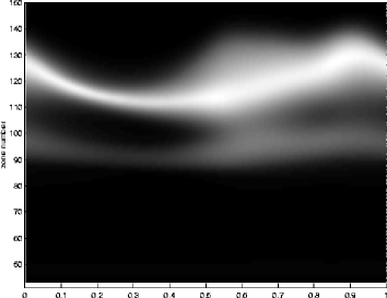
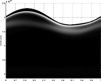
Figure 1.: Time dependence of turbulent energy during the pulsation cycle. Left: vs. zone index, right: vs. Lagrangean radius.

Turbulence and convection are inherently 3D phenomena. While a great deal of progress has been made in 3D simulations, it remains very difficult to model astrophysically realistic conditions which have very large Rayleigh numbers Ra$\approx$ 10¹², and very small Prandtl numbers Pr$\approx$ 10^-6. It is of course even more difficult to incorporate them in stellar models (see however the solar models of Nordlund & Stein at this meeting).

Large amplitude stellar pulsations increase the difficulties by involving time dependence. Indeed, the source regions occur in the partial ionization regions of hydrogen, helium and Fe-group atoms, and these features are neither Lagrangean (they move through the fluid) nor Eulerian (they move through space). Fig. 1 shows the behavior of the turbulent energy $e_{t}$ over a period in a pulsating Cepheid model with a period of 10.9 days ($M$=6.1M_⊙, $L$=3377L_⊙, $T_{ef\!f}$=5207K, $X$=0.70, $Z$=0.02). Similar behavior occurs in RR Lyrae models, but we concentrate here on Cepheids which are actually more daunting numerically because of the sharpness of their H ionization front. On the right side we display $e_{t}$ as a function of Lagrangean radius. The lightness of the grey reflects the strength of $e_{t}$. On the left, Fig. 1 displays $e_{t}$ as a function of zone index, i.e. as attached to the Lagrangean mass coordinate, i.e. in the fluid frame. The turbulent energy is largest in the region associated with the combined H and first He ionization fronts. The next most important region of turbulent energy is the He⁺–He⁺⁺. There can also be turbulent energy in the Fe group partial ionization regions, at least for Galactic metallicity, but is comparatively weak and does not show up on the scale of the figure. Fig. 1 clearly shows how the turbulent energy tracks the source regions which move through the fluid during the pulsation. It also shows the importance of time dependence in the convective pulsating envelope. Both figures show that the turbulent energy increases during the pulsational compression phase and that the two turbulent zones briefly merge.

Fig. 2 shows the temporal behavior of the convective flux in the frame of the zone index (Lagrangean) and in the stellar frame, respectively, and can be compared to the turbulent energy in Fig. 1. The convective flux exists only in the regions of negative entropy gradient regions ($Y>0$, cf. Eq. 6) and is therefore confined to narrower regions than the turbulent energy which can diffuse outside these regions.

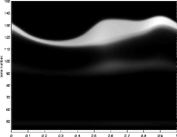
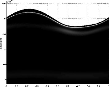
Figure 2.: Convective luminosity; left: vs. zone index, right: vs. Lagrangean radius.

Attempts at including convection in pulsation codes are actually not new. Castor (1971) was the first to present a nonlocal time dependent formulation and numerical application to a pulsating stellar envelope model. Later, Stellingwerf simplified Castor’s formulation and performed a number of model calculations (Stellingwerf 1982, Bono & Stellingwerf 1994). Similar turbulent convective model equations have been used by Gehmeyr and Winkler (1992). Another early computation of linear convective models is that of Gonczi & Osaki (1980).

2. The Turbulent Convection Recipe

$${du\over dt}=-{1\over\rho}{\partial\over\partial r}\left(p+p_{t}+p_{\nu}\right)-{GM_{r}\over r^{\scriptstyle 2}}\,,$$ (1)

$${d\over dt}\left(e+e_{t}\right)=-{\left(p+p_{t}+p_{\nu}\right)\over\rho}\ {1\over r^{\scriptstyle 2}}{\partial r^{\scriptstyle 2}u\over\partial r}-{1\over\rho r^{\scriptstyle 2}}{\partial\over\partial r}\left[r^{\scriptstyle 2}\left(F_{c}+F_{t}+F_{r}\right)\right]\,,$$ (2)

$${de_{t}\over dt}=-{1\over\rho r^{\scriptstyle 2}}{\partial\over\partial r}\left(r^{\scriptstyle 2}F_{t}\right)-{e^{\scriptscriptstyle 1/2}_{t}\over\Lambda}\alpha_{d}\thinspace\left(e_{t}-S_{t}\right)-{\left(p_{t}+p_{\nu}\right)\over\rho}\ {1\over r^{\scriptstyle 2}}{\partial r^{\scriptstyle 2}u\over\partial r}\,,$$ (3)

$$p_{t}=\alpha_{p}\thinspace\rho\thinspace e_{t}\thinspace,\quad\quad\quad p_{\nu}=-\alpha_{\nu}\thinspace\rho\Lambda e^{\scriptscriptstyle 1/2}_{t}{\partial u\over\partial r}\,,$$ (4)

$$F_{t}=-\alpha_{t}\thinspace\rho\Lambda{2\over 3}{\partial\thinspace\thinspace e_{t}^{{\scriptscriptstyle 3/2}}\over\partial r},\quad\quad F_{c}=\alpha_{c}\alpha_{\Lambda}\thinspace\rho e_{t}^{{\scriptscriptstyle 1/2}}\thinspace c_{p}T\thinspace Y\,,$$ (5)

$$S_{t}=\alpha_{s}\thinspace\alpha_{\Lambda}\thinspace(e_{t}\thinspace{p\over\rho}\thinspace\beta T\thinspace Y)^{{\scriptscriptstyle 1/2}},\ \ \ \ \ Y=\left[-{H_{p}\over c_{p}}{\partial s\over\partial r}\right]_{+}\,,$$ (6)

where $p$ is the gas pressure, $\beta$ is the thermal expansion coefficient, $\Lambda=\alpha_{\Lambda}\thinspace H_{p}$, and $H_{p}=p\thinspace r^{\scriptstyle 2}/(\rho GM)$ is the pressure scale height, and other symbols have their usual meanings.

This scheme gives rise to an unphysical behavior at the boundaries of the convective regions where $Y\rightarrow 0$. Because $\delta S_{k}\propto\delta Y/\sqrt{Y}$ the linearization has a pole there that shows up in the growth rates along sequences of models when the zoning is very fine or the mesh happens to fall on a point with small $Y$.

This difficulty can be avoided with an alternative model equation for the source which is more in line with the Gehmeyr–Winkler formulation (1992)

$$S_{t}=(\alpha_{s}\thinspace\alpha_{\Lambda})^{\scriptstyle 2}\thinspace\thinspace{p\over\rho}\thinspace\beta T\thinspace\thinspace Y\,,$$ (7)

For comparison, in Fig. 3, we show the effect that the two formulations have on the linear growth rates for a sequence of Cepheid models ($M$=6.75M_⊙, $L$=4843, $X$=0.70, $Z$=0.02, variable $T_{ef\!f}$). The difference is seen not to be substantial, although the alternate $S_{t}$ increases the maximum period that unstable overtone models can have (cf. Fig. 12 and 13 in YKB). For this model we have taken the parameters ($\alpha_{d}=1.0,\alpha_{c}=2.25,\alpha_{s}=0.75,\alpha_{\nu}=1.8,\alpha_{t}=0.25,\alpha_{p}=0.667,e_{0}=1.e4,\alpha_{\Lambda}=0.4$). These values are used for illustrative purposes. Except for this one example we have not yet explored the general effects of using expression (7). We are also still in the process of calibrating the $\alpha$’s using the best available astrophysical constraints.

Figure 3.: Fundamental and first overtone growth rates for a Cepheid sequence. Solid line: formulation of Eq. 6, dotted line: Eq. 7.

3. Work Integrand

It is interesting to see how turbulent convection affects the stability of the pulsational modes. Turbulent convection actually affects the stability in two ways, indirectly, by altering the structure of the equilibrium model and, directly, in the linearization of the equations. (cf. e.g. Yecko, Kolláth & Buchler 1998, YKB hereafter).

The work done on the pulsation per cycle is given by

$$W=\oint dt\thinspace\thinspace\bigl{(}\int dm\thinspace p{dv\over dt}\bigr{)},$$ (8)

where the total pressure $p=p_{g}+p_{t}+p_{\nu}$ is composed of the separate contributions of the gas (and radiation) pressure $p_{g}$, the turbulent pressure $p_{t}$ and the eddy viscous pressure $p_{\nu}$. If we denote the linear eigenvalues by $\sigma=i\omega+\kappa$, for an assumed exp($\sigma t$) dependence, then the relative growth rate is given by

$$\eta=2{\kappa\over\omega}={2\pi\over\omega^{\scriptstyle 2}I}\thinspace\thinspace{\rm Im}\int\delta p\delta v^{*}\thinspace dm\thinspace,$$ (9)

$$I=\int|\delta r|^{\scriptstyle 2}\thinspace dm\thinspace,$$ (10)

and the $\delta$ refer to the pressure, specific volume and radial displacement parts of the modal eigenvector, respectively, and $I$ is the moment of inertia of the mode.

The quantity $\eta$ represents the energy growth of a mode over one period, equal to the inverse of the quality factor $Q$ that is commonly associated with resonant electronic devices.

Here we illustrate with a fundamental Cepheid model (with M=5.2M_⊙, L=3293L_⊙, $T_{ef\!f}$=5677 K, X=0.716, Z=0.01) how the work integrands are affected by convection. It is of interest to see how the various regions contribute to the work, as well as how the turbulent convective quantities affect the stability.

In Fig. 4 we display the linear work integrand (thick solid line) together with the separate contributions: gas pressure (thin solid line), $p_{t}$ (dotted line) and $p_{\nu}$ (dashed line). The area under the curve is slightly positive since the mode is linearly unstable. As expected, the eddy pressure is everywhere damping. The turbulent pressure, on the other hand, can be both driving or damping depending on its phase with respect to the density variations. The sharp peak is associated with the H and first He ionization, whereas the broad peak is due to the second He ionization and the tiny peak to Fe.

Figure 4.: Linear Work Integrand (surface to the right) showing separate contributions of the gas, turbulent and eddy viscosity pressures.

Figure 5.: Nonlinear Work Integrand (surface to the right) showing separate contributions of the gas, turbulent and eddy viscosity pressures.

The total work (Eq. 8) that is done over a limit cycle is zero, but again it is of interest to see how nonlinear effects change the nonlinear work integrand which is displayed in Fig. 5. Our nonlinear work integrand is arbitrarily normalized by twice the nonlinear pulsational kinetic energy. The figure shows the separate contributions of $p_{g}$, $p_{t}$ and $p_{\nu}$. Here there is, in addition, a pseudo-viscous pressure whose contribution is very small compared to that of the other pressures and is not shown here.

In comparison to the linear work integrand, most noticeable are (a) the broadening of the driving region because the (non Lagrangean) ionization fronts sweep through the envelope during the pulsation; this is already known from purely radiative models (e.g. Figs. 4 and 7 in Buchler 1990) and (b) the greatly enhanced damping by the eddy viscosity pressure $p_{\nu}$.

A final comment concerning frequently made approximations. In many early pulsation computations convection was assumed to be ’frozen in’: Convection was included in the computation of the equilibrium model, but all convective quantities were held constant in the calculation of the period and of the linear growth rates. A similar approximation is often made in stellar evolution computations. In YKB we have examined this approximation and found it to be very lacking. The perturbation of the turbulent quantities, and concomitantly of the convective flux, has a very strong damping effect on the pulsation.

In Fig. 6 we summarize these results for a $T_{ef\!f}$sequence of models (with $M$=5M_⊙, $L$=2060L_⊙) for the fundamental and first overtone modes. The solid lines represent the exact growth rates (i.e. correct linearization of all quantities). The line with crosses represents the ’frozen convection’ approximation which is seen to be inadequate. The fundamental instability strip (the domain where the modal growth rate is positive) is enormously broadened and shifted. For the overtone the effect appears even more drastic. The mode, which is stable throughout the whole temperature region, now becomes unstable over a very broad region.

The dotted line corresponds to the approximation of ’adiabatic’ convection, i.e. $T\delta s_{t}$ $\equiv$ $\delta e_{t}-p_{t}\delta v=0$. Physically it corresponds to assuming that all convective time scales are very long. This approximation is seen to underestimate somewhat the damping effects of convection.

Another convenient approximation is the other extreme, which is to assume that all convective time scales are very short compared to the other time scales, i.e. from Eq. 3 we obtain

$${\partial\over\partial r}\left(r^{\scriptstyle 2}F_{t}\right)-{e^{\scriptscriptstyle 1/2}_{t}\over\Lambda}\alpha_{d}\thinspace\left(e_{t}-S_{t}\right)=0.\,,$$ (11)

This is seen to be the best of the approximations. It is also the simplest to apply in evolutionary calculations in which a time independent, local mixing length recipe is used (which would correspond here to setting in addition $F_{t}=0$ or $\alpha_{t}=0$, i.e. no diffusion of turbulent energy).

Figure 6.: Effects of commonly made approximations on position of red and blue edges; left: fundamental mode, right: first overtone.

4. Nusselt vs. Rayleigh Numbers

The Nusselt number is defined as Nu=$F_{c}/F_{cond}$, where in our case the conductive flux is the radiative flux, and the Rayleigh number is Ra=$g\beta d^{3}TY/(\nu\chi)$. Here $g$ is the local gravity, $d$ is the local scale height, $\nu$ is the kinematic viscosity and $\chi$ is the radiative conductivity. There is general agreement that Nu should depend on Ra, viz. Nu = Ra ^a, but there is no theoretical agreement on what the value of $a$ should be (e.g. Spiegel 1971). Some experimental results indicate that $a=0.28$ (Castaing et al. 1989), but it is not clear that they should apply to the stellar case where the boundaries can adjust to accommodate a fixed stellar luminosity, and where the physical quantities have strong spatial variations, especially through the partial ionization zones.

Figure 7.: Left: Local Nusselt versus Rayleigh number. Right: Péclet Number in two Cepheid envelopes.

In Fig. 7 we reproduce that behavior of the local Nu versus Ra numbers throughout the convective regions of the two typical Cepheid models $M$=5M_⊙, $L$=2090L_⊙, $T_{ef\!f}$=4900 (solid line) and 5300K (dotted) of YKB. Only the combined H–He convective regions, where Nu$>1$, are shown. For reference we have shown two thin lines with slopes 1/2 and 1/3, respectively. Throughout the convective region the exponent $a$ varies between 0.45 and 0.53, and thus agrees best with the higher theoretical value of 1/2 (Spiegel 1971). The right hand side shows the Péclet number defined as the ratio of the thermal diffusion time scale to the convective time scale.

5. Sequence of Cepheid models

YKB performed some sensitivity tests of the properties of Cepheid models obtained with the 1D turbulent convective model. Here we just add Fig. 8 which displays the strength of the convective luminosity as a function of zone number (bottom scale), for a sequence of Cepheid models starting from the blue edge in front, to the red edge in the back. The importance of the convective flux increases from the blue edge, where it is relatively unimportant, to the red edge. The H and first He ionization regions are always merged into a single zone. Near the blue edge the second ionization region for He forms a separate convective region, but when we arrive at the red edge, convection encompasses both H and He regions, and almost joins with Fe region (left).

Figure 8.: Profiles of the ratio of convective to total luminosity along a sequence; blue edge in front (bottom) and red edge towards the back (top).

6. Double-Mode (DM) Pulsations

The numerical modelling of double mode (DM) pulsations has been a long standing quest in which purely radiative models have failed. In a recent paper (Kolláth et al. 1998, hereafter KBBY) it was shown that with the inclusion of turbulent convection DM pulsations appear almost naturally in Cepheid models. Almost concomitantly, but independently, Feuchtinger (1998) found DM behavior in RR Lyrae pulsations which we have since also confirmed. KBBY described the behavior of the DM Cepheids in terms of truncated amplitude equations (Eqs. 1 of KBBY), and they appeared to give excellent agreement with the model that was studied.

Fig. 1 of KBBY showed the transient evolutions for a given Cepheid model and for different initializations of the hydrocode. The evolution toward a DM pulsational state is clearly exhibited. The results of the pulsational states of a number of Cepheid models were summarized in a bifurcation diagram (Fig. 4 of KBBY). The DM states were obtained with the regular hydrodynamics code after lengthy time integrations with suitable initial conditions. The single mode pulsational states, whether stable or not, were obtained with Stellingwerf’s relaxation method (cf. Kovács & Buchler 1987), sometimes with a lot of perseverance.

When such models were more carefully scrutinized it became apparent that a different transient evolution was possible (Kolláth et al. 1999), namely toward the F limit cycle on the bottom right. This situation is shown in Fig. 9. It is clear that in addition to the stable DM there must coexist a stable F limit cycle and a second unstable DM.

     

Figure 9.: Transient evolution of Cepheid model. Left (right): the F amplitude – O1 amplitude plane; right: energy plane The trajectories correspond to various initializations.

This new development forces us to also reconsider the bifurcation diagram (Fig. 4 of KBBY). We had suggested that the sharp vertical rise (drop) of the fundamental (overtone) amplitudes was due to the presence of a pole in the discriminant ${\cal D}$. While such a pole is present it turns out to be too far away (in $T_{ef\!f}$) to cause the observed vertical slope. Upon closer inspection it has been found (Kolláth et al. 1999) that the bifurcation diagram is a bit more complicated than first thought. Fig. 10 is an adaptation of the results of Kolláth et al. (1999).

Figure 10.: Bifurcation diagram for the Cepheid model sequence; Solid/open circles: F and O1 limit cycles, Squares: F and O1 component amplitudes of double mode cycles.

Indeed, the region of fundamental mode pulsations extends to the left into the region where DM pulsations can occur. There is thus a narrow region of hysteresis where both F and DM pulsation can occur. We note immediately that this bifurcation structure, in particular the hysteresis, cannot be accommodated with the amplitude equations of KBBY that were truncated at the $A^{3}$ terms.

Figure 11.: The fixed point solutions as a function of the control parameter $\lambda$. Solid dots for stable, open circles for unstable fixed points.

Kolláth et al. (1999) show that one can readily get agreement by adding the most important next order terms in the truncation, which normal form theory shows to be $-r_{0}A_{0}^{5}$ and $-r_{1}A_{1}^{5}$. (We disregard the additional quintic cross-coupling terms).

$${d\thinspace A_{0}\over dt}=\bigl{(}\kappa_{0}-q_{00}A_{0}^{2}-q_{01}A_{1}^{2}\thinspace-r_{0}A_{0}^{\scriptstyle 4}\bigr{)}\thinspace\thinspace A_{0}$$ (12)

$${d\thinspace A_{1}\over dt}=\bigl{(}\kappa_{1}-q_{10}A_{0}^{2}-q_{11}A_{1}^{2}\thinspace-r_{1}A_{1}^{\scriptstyle 4}\bigr{)}\thinspace\thinspace A_{1}$$ (13)

Rather than using amplitudes $A$, it is equivalent and perhaps more convenient here to introduce the ’energies’, $e=A^{\scriptstyle 2}$, instead of the amplitudes $A$. The amplitude equations, with the new terms added, take on the form

$${d\thinspace e_{0}\over dt}=2\thinspace\bigl{(}\kappa_{0}-q_{00}e_{0}-q_{01}e_{1}\thinspace-r_{0}e_{0}^{\scriptstyle 2}\bigr{)}\thinspace\thinspace e_{0}$$ (14)

$${d\thinspace e_{1}\over dt}=2\thinspace\bigl{(}\kappa_{1}-q_{10}e_{0}-q_{11}e_{1}\thinspace-r_{1}e_{1}^{\scriptstyle 2}\bigr{)}\thinspace\thinspace e_{1}$$ (15)

The loci of the fixed points are obtained by setting the RHSs of these equations equal to zero. Without the $r$ terms these nullclines (other than the two coordinate axes) are simply straight lines that intersect at most once, and when they intersect they give the DM as has been known for a long time (Buchler & Kovács 1986). Clearly no hysteresis is possible in this case. On the other hand, even with small $r$ values the lines bend and multiple intersections become possible.

This situation is depicted in Fig. 11. For the sake of illustration, we have chosen the numerical values ($q_{00}$=2.179e-3, $q_{01}$=4.5e-3, $q_{10}$=5.9e-3, $q_{11}$=16.e-3, $r_{0}$=–3.e-4, $r_{1}$=1.4e-3), for simplicity keeping these values constant even though in a real sequence of models they would vary. The variation of the growth rates along a sequence is more important and we assume that $\kappa_{0}=\bar{\kappa}_{0}$ + 0.8e-3$\lambda$, $\kappa_{1}=$ $\bar{\kappa}_{1}$ + 1.6e-3 $\lambda$, where $\bar{\kappa}_{0}$=2.e-3, $\bar{\kappa}_{1}$=7.5e-03. The parameter $\lambda$ varies between 0 and 1 along this sequence.

Figure 12.: Bifurcation diagram corresponding to the illustrative example. Amplitudes of the SM and DM limit cycles. The stable (unstable) limit cycles are denoted by thick (thin) dots.

The corresponding bifurcation diagram is presented in Fig. 12. It is seen to display the same general features as the actual Cepheid diagram. In particular, it has an single-mode O1 regime up to $\lambda\sim$ 0.08, a DM regime from $\lambda\sim$ 0.08–0.90, and a coexistence between DM and F modes from $\lambda\sim$0.67–0.90. To the right $\lambda\,\raise 2.0pt\hbox{$>$}\kern-8.0pt\lower 2.0pt\hbox{$\sim$}\,$ 0.90, only the F mode LC is stable. Note that the annihilation of the stable and unstable DMs that occurs at $\lambda\sim$ 0.90 gives rise to the vertical observed tangent.

Note that the complexity of the bifurcation diagram is partly due to the values we have chosen for the control parameters, $T_{ef\!f}$ and $\alpha_{\nu}$. Our values correspond to realistic Cepheids and are not idealized for the purpose of clarifying the evolution into single and double modes. If we had chosen instead to unravel the complete nature of the bifurcation, we would have been forced to choose both $T_{ef\!f}$ and $\alpha_{\nu}$ to correspond to the polycritical point – where the F, O, DM and the trivial solution coexist (this point was previously discussed in KBBY and plotted there in Fig. 3). Near to this point the dynamics is given by the cubic equations (we can take this as the definition of near). Furthermore, the bifurcation structure is straightforward once we know how we move through the parameter space given by $T_{ef\!f}$ and $\alpha_{\nu}$. (This is not true if the bifurcation is subcritical, but as yet we have not encounterd this case). For a more general unfolding of the bifurcation, however, this ideal picture is easily extended beyond its reach. So we ought to expect that some effects of this breakdown, in the form of an increasing nonlinearity, will begin to appear. What we seem to be witnessing here is, in fact, the need for quintic terms as the polycritical point becomes more distant.

7. Conclusions

It is perhaps remarkable that such a simple 1D recipe for turbulent convection can give such drastic improvements over purely radiative codes. It may indicate that, at least for Cepheid and RR Lyrae variables, this recipe incorporates all the physics of turbulence and convection that is essential to model these pulsations. It is possible that a nonlocal, time dependent dissipation which this model equation provides is all that is needed.

We are only at the beginning of the process of calibrating the seven $\alpha$ parameters that appear in the turbulent convective description. There are numerous constraints that need to be satisfied, and we hope that despite the large number of these $\alpha$’s these constraints can be satisfied. In particular it will be a challenge to obtain the observational properties of both the Galactic and of the Magellanic Cloud variable stars. Only then will we know whether our simple 1D model is adequate.

Acknowledgments.

We wish to thank the organizers for a most pleasant and fruitful meeting. This work has been supported by NSF (AST95–28338).

References

Antonello, E. & Poretti, E. Reduzzi, L, 1990, AA 236, 138

Beaulieu, J.P. et al. 1995, AA 303, 137

Beaulieu, J.P. & Sasselov, D. 1997, in 12^th IAP Coll. Variable Stars and the Astrophysical Returns of Microlensing Surveys, Eds. R. Ferlet & J.P. Maillard

Bono, G., Stellingwerf, R.F. 1994, ApJ Suppl 93, 233–269

Buchler J.R. 1990, in The Numerical Modelling of Stellar Pulsations; Problems and Prospects, Ed. J.R. Buchler NATO ASI Ser. C302 (Dordrecht: Kluwer), 1.

Buchler, J. R. 1993, Nonlinear Phenomena in Stellar Variability, (Dordrecht: Kluwer), repr. from ApSpS 210, 1 (1993)

Buchler, J.R., Kolláth, Z., Beaulieu, J.P., Goupil, M.J., 1996, ApJLett 462, L83

Buchler, J.R. & Kovács, Z. 1986, ApJ 308, 661

Buchler, J. R. 1998, in A Half Century of Stellar Pulsation Interpretations: A Tribute to Arthur N. Cox, eds. P.A. Bradley &J.A. Guzik, ASP 135, 220

Castaing, B. et al. 1989, J. Fluid Mech. 204, 1

Castor, J. I. 1971, ApJ, 166, 109

Feuchtinger, M. 1998, AA 322, 817

Gautschy, A. & Saio, H. 1995, ARAA 33, 75 and 1996, ibid. 34, 551

Gehmeyr, M. , Winkler, K.-H. A. 1992, AA 253, 92–100; ibid. 253, 101–112

Gonczi, G. & Osaki, Y. 1980, AA 84, 304

Kolláth, Z., Beaulieu, J.P., Buchler, J. R. & Yecko, P., 1998, 502, L55 [KBBY]

Kolláth, Z., Buchler, J. R., Yecko, P. Szabó, R. & Csubry, Z. 1999 (in preparation)

Kovács, G. & Buchler, J.R. 1987, ApJ 324, 1026

Moskalik, P., Buchler, J.R. & Marom, A. 1992, ApJ 385, 685

Spiegel, E. A. 1971, Comments on Astrophysics 53

Stellingwerf, R.F. 1982, ApJ 262, 330

Welch, D. et al. 1995, in Astrophysical Applications of Stellar Pulsation, IAU Coll. 155, ed R.S Stobie (Cambridge, University Press)

Yecko, P., Kolláth Z., Buchler, J. R. 1998, A&A 336, 553 [YKB]