Growth and saturation of the Kelvin-Helmholtz instability with parallel and anti-parallel magnetic fields

Abstract

We investigate the Kelvin-Helmholtz instability occuring at the interface of a shear flow configuration in 2D compressible magnetohydrodynamics (MHD). The linear growth and the subsequent non-linear saturation of the instability are studied numerically. We consider an initial magnetic field aligned with the shear flow, and analyze the differences between cases where the initial field is unidirectional everywhere (uniform case), and where the field changes sign at the interface (reversed case). We recover and extend known results for pure hydrodynamic and MHD cases with a discussion of the dependence of the non-linear saturation on the wavenumber, the sound Mach number, and the Alfvénic Mach number for the MHD case.

A reversed field acts to destabilize the linear phase of the Kelvin-Helmholtz instability compared to the pure hydrodynamic case, while a uniform field suppresses its growth. In resistive MHD, reconnection events almost instantly accelerate the buildup of a global plasma circulation. They play an important role throughout the further non-linear evolution as well, since the initial current sheet gets amplified by the vortex flow and can become unstable to tearing instabilities forming magnetic islands. As a result, the saturation behaviour and the overall evolution of the density and the magnetic field is markedly different for the uniform versus the reversed field case.

1 Introduction

The Kelvin-Helmholtz (KH) instability occurs at the interface between two fluids or plasmas moving in opposite directions. Pioneering studies were made by Chandrasekhar (1961). As shear flows are present in many astrophysical situations, the KH instability receives continuous attention in the astrophysics literature. In solar coronal loops, shear flows arise in the vicinity of a resonant radius when the magnetized loop is perturbed at a frequency which matches the characteristic Alfvén frequency at this radius. Recent studies address whether these shear flows are KH unstable ([Karpen et al. (1994)]; [Poedts et al. (1997)]). In the heliosphere, the solar wind flows past planetary magnetospheres, and instabilities may occur at bow shocks or further out in the magnetotails (see, e.g. [Uberoi (1984)]). Similarly, KH instabilities are studied at the heliopause, where the solar wind is halted and meets the interstellar medium ([Chalov (1996)]). Numerous observations of extragalactic jets inspired research into the KH instability taking relativistic effects into account. A recent example is found in [Hanasz and Sol (1996)].

We investigate both the linear and the non-linear regime of the KH instability for compressible hydrodynamic (HD) and magnetohydrodynamic (MHD) cases. Our numerical study makes use of the Versatile Advection Code (VAC) for solving the fluid equations, developed by Tóth (1996, 1997). This code can be used as a convenient tool to handle hydrodynamic and magnetohydrodynamic one-, two-, or three-dimensional problems in astrophysics (see [Keppens and Tóth (1998)]). We perform all our calculations in two dimensions.

First, we briefly summarize important findings preceding and augmenting our study. Theoretical studies of the KH instability started with the linear stability analysis of [Chandrasekhar (1961)] for incompressible HD and MHD cases. It was noted how a uniform magnetic field, parallel to the shear flow, completely stabilizes the KH instability when the velocity jump across the shear layer is less than twice the Alfvén speed. [Blumen (1970)] extended the linear study to the hydrodynamic compressible case and found instability when the sound speed exceeds half the velocity jump. In our investigation, we will therefore restrict attention to cases where half the total velocity jump is below the sound speed, but above the Alfvén speed. The extension of these linear studies to compressible MHD cases is found in [Miura and Pritchett (1982)]. While the magnetic field was taken to be uniform, they allowed for magnetic fields and wavenumbers with arbitrary orientations in the plane perpendicular to the velocity gradient. Since we restrict ourselves to 2D configurations, our linear results for uniform magnetic fields parallel to the shear flow recover their findings. In particular, we similarly study variations with wavenumber, sound Mach number and magnetic field strength. We extend their findings by discussing the further non-linear evolution as well. In addition, we simulate the KH instability when the initial field is anti-parallel (or reversed) in both opposite flowing plasma layers.

Recently, [Frank et al. (1996)] carried out non-linear 2D MHD calculations for two cases. They took the field parallel to the shear flow and compared the KH evolution of a ‘weak’ field case with a ‘strong’ field case. The velocity jump across the shear layer equaled the sound speed, and amounted to 5 and 2.5 times the Alfvén speed, respectively. It was found that the magnetic tension also stabilizes the non-linear regime for these two cases. We confirm and extend this result for the uniform field over a wider range of Alfvén and sound Mach numbers. [Frank et al. (1996)] found that numerical dissipation, mimicking viscous and resistive effects, eventually led to similar end states consisting of a stable laminar flow with dynamically aligned velocity and magnetic fields.

A systematic numerical study of the 2D uniform case in MHD was done by Malagoli et al. (1996). They varied the ratio of the Alfvén speed to the sound speed, and could generally identify three stages in the instability. They referred to these stages as the linear stage, the dissipative transient stage with intermittent reconnection events, and the saturation stage where small scale turbulent motions decay to form aligned structures. Their final stage is qualitatively similar to the laminar flow end state of [Frank et al. (1996)]. We focus attention to the two stages preceding turbulence, where the amplification and the dynamic influence of the magnetic field grows and eventually halts the KH instability.

The main extension presented here is a consideration of the reversed field case in 2D compressible MHD. There, new physical effects emerge as reconnection can occur earlier in the evolution of the KH instability. We compare this reversed case with the pure hydrodynamic and uniform magnetohydrodynamic case. Independent investigations by [Dahlburg et al. (1997)] studied similar ‘current-vortex’ sheets where both the initial velocity and the magnetic field are given by hyperbolic tangent profiles. By considering relatively strong fields, these authors could investigate resistive instabilities, modified by the KH flow. We show how the KH instability in the presence of an initially weak reversed field can induce tearing instabilities. Their study was done in incompressible visco-resistive MHD, so we extend their results by adding compressibility. Another important difference is that we take a discontinuous field reversal at the shear flow interface, while [Dahlburg et al. (1997)] took the ratio of the magnetic shear width to the velocity shear width around unity. We have therefore investigated the dependence on the initial magnetic field configuration. This also allows a more detailed comparison with the incompressible studies of ‘current-vortex’ sheets. The most recent study by [Dahlburg (1998)] considers nonlinear effects analytically, under the assumptions of incompressibility, while neglecting higher harmonics and the distortion of the fundamental disturbance. Our numerical study allows us to relax these assumptions to fully 2D compressible situations.

The manuscript is built up as follows: in section 2 we list the conservation laws, summarize the initial conditions, and we give a brief discription of the KH instability. The numerical method is outlined in section 3. The results are split into a discussion of the linear regime (section 4) and an in depth study of the non-linear saturation behaviour (section 5). We end with a discussion and conclusions in section 6.

2 Conservation laws and initial configuration

The MHD equations are written in conservation form. The conservative variables are density $\rho$, momentum $\rho\mbox{\bf v}$, energy density $\cal{E}$, and the magnetic field B. The conservation of mass is simply written as

$$\frac{\partial\rho}{\partial t}+\nabla\cdot(\rho\mbox{\bf v})=0.$$ (2.1)

The evolution equation for the momentum density $\rho\mbox{\bf v}$ reads

$$\frac{\partial(\rho\mbox{\bf v})}{\partial t}+\nabla\cdot[\rho\mbox{\bf v}\mbox{\bf v}+p_{tot}I-\mbox{\bf B}\mbox{\bf B}]=0,$$ (2.2)

where $\rho\mbox{\bf v}\mbox{\bf v}$ is the Reynolds stress tensor, $p_{tot}=p+\frac{1}{2}B^{2}$ is the total pressure, and $I$ is the identity tensor. The thermal pressure $p$ is related to the energy density as $p=(\gamma-1)({\cal{E}}-\frac{1}{2}\rho v^{2}-\frac{1}{2}B^{2})$. We set the adiabatic gas constant $\gamma$ equal to $5/3$. The magnetic part of Maxwell’s stress tensor is $\frac{1}{2}B^{2}I-\mbox{\bf B}\mbox{\bf B}$. Magnetic units are defined such that the magnetic permeability is unity. The induction equation is

$$\frac{\partial\mbox{\bf B}}{\partial t}+\nabla\cdot(\mbox{\bf v}\mbox{\bf B}-\mbox{\bf B}\mbox{\bf v})=\eta\nabla^{2}\mbox{\bf B}.$$ (2.3)

Ideal MHD corresponds to a zero resistivity $\eta$ and ensures that magnetic flux is conserved. In resistive MHD, field lines can reconnect. The energy equation we use is

$$\frac{\partial{\cal{E}}}{\partial t}+\nabla\cdot({\cal{E}}\mbox{\bf v})+\nabla\cdot(p_{tot}\mbox{\bf v})-\nabla\cdot(\mbox{\bf v}\cdot\mbox{\bf B}\mbox{\bf B})=\nabla\cdot\left[\mbox{\bf B}\times\eta(\nabla\times\mbox{\bf B})\right].$$ (2.4)

In resistive MHD ($\eta>0$), the right hand side contains the Ohmic heat term $\eta(\nabla\times\mbox{\bf B})^{2}$, which is a source of internal energy.

We solve the above set of non-linear ideal MHD equations as an initial value problem in two spatial dimensions. We consider a Cartesian two-dimensional rectangular grid with $0\leq x\leq L_{x}$ and $-L_{y}\leq y\leq L_{y}$. We take $L_{y}$ as our unit of length. The initial pressure $p_{0}$ and density $\rho_{0}$ are set to unity throughout the domain and thus define our normalization.

We distinguish between the following three cases: (i) a purely hydrodynamic case with $B=0$ at all times; (ii) a ‘uniform’ MHD case where the magnetic field at $t=0$ is set to $B_{0}\hat{x}$ everywhere; and (iii) a ‘reversed’ MHD case where the magnetic field at $t=0$ is $-B_{0}\hat{x}$ for $y>0$ and $B_{0}\hat{x}$ for $y<0$. The reversed case must be seen as a limiting case of a continuous field reversal, where $B_{x}=B_{0}\tanh(y/b)$ and $b\rightarrow 0$. We will explicitly discuss this connection with an initially smooth current sheet. Note that when $b\neq 0$, we have a non-constant initial pressure $p(y)$ from total pressure equilibrium.

We apply a shear velocity in the $x$-direction with amplitude $V_{0}$, of the form $v_{x}=V_{0}\tanh(y/a)$. The width of the ‘inner’ region where the velocity reverses is always set to $a=0.05$. In order to guarantee instability ([Chandrasekhar (1961)], [Blumen (1970)], [Miura and Pritchett (1982)]) we vary the amplitude of the shear such that

$$B_{0}/\sqrt{\rho_{0}}\equiv v_{a}<V_{0}<c_{s}\equiv\sqrt{\gamma p_{0}/\rho_{0}}.$$ (2.5)

The sound speed $c_{s}$ and the Alfvén speed $v_{a}$ are used to define the sound Mach number $M_{s}\equiv V_{0}/c_{s}$ and the Alfvénic Mach number $M_{a}\equiv V_{0}/v_{a}$, respectively. We perturb this initial configuration with a velocity component perpendicular to the background shear velocity of the form $\delta v_{y}=v_{y0}\sin(k_{x}x)\exp{[-y^{2}/\sigma^{2}]}$. We take the amplitude of this velocity perturbation $v_{y0}=0.0001$, which is always much smaller than the shear velocity $V_{0}$. The Gaussian component of the velocity perturbation $\delta v_{y}$ has a parameter $\sigma$, representing the decay of the amplitude $v_{y0}$ in the outer region $|y|>a$, and the ratio $\sigma/a$ is set to 4 in our calculations.

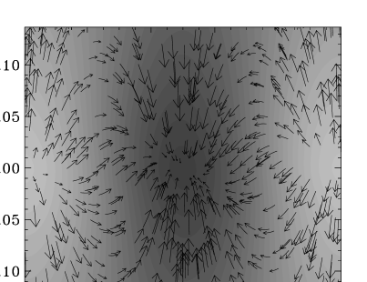
Figure 1: The structure of the KH instability. The inner region containing the background shear velocity is $|y|<a=0.05$. We show the density perturbation resulting from the initial velocity perturbation (bright is higher density, dark corresponds to lower density). Also shown is the induced pressure gradient force field which enhances the initial vertical displacement in the centre of the layer.

With these initial conditions and the use of periodic boundary conditions in the $x$-direction, we can simulate the development of a KH instability at certain Mach number and wavenumber $k_{x}=2\pi/L_{x}$. The driving force behind the KH instability and its resulting spatial structure is easily understood from Fig. 1 (see also the schematic Fig. 2 in [Miura and Pritchett (1982)]).

Consider first what happens in the inner region $|y|<a$ containing the background shear velocity. When we impose a sinusoidal perturbation $\delta{v_{y}}\sim\sin(k_{x}x)$ at $y=0$, the velocity shear $v_{x}^{\prime}=dv_{x}/dy$ in the equilibrium flow produces a force $-\rho v_{x}^{\prime}\delta v_{y}$ in the $x$-direction, such that acceleration of the plasma in the peaks of the sine wave is anti-parallel to the one felt in the throughs. The resulting density perturbation is a periodic depletion and enhancement as shown in Fig. 1, which is horizontally displaced from the imposed velocity perturbation. The pressure perturbation follows the density perturbation, and sets up a pressure gradient force that enhances the initial vertical displacement within $|y|<a$. The pressure gradient force is indicated by the arrows in Fig. 1. Note how in the inner region, the pressure gradient is in phase with the initial velocity disturbance (from bottom to top in the left half of the figure, and from top to bottom in the right half). Hence, the situation is inherently unstable.

The situation is different in the outer region $|y|>a$. There, the imposed sinusoidal perturbation is damped by $\exp{[-y^{2}/\sigma^{2}}]$, and the background flow is essentially uniform. The pressure gradient force is out of phase with the initial flow perturbation. The net result is a clock-wise plasma circulation around the central density depletions. Matter pushed out by the excess pressure created in the central layer which reaches $y=+a$ gets entrailed to the right by the background flow and is pulled towards the central layer again at the throughs of the initial perturbation.

3 Numerical method

All calculations are performed with the Versatile Advection Code (VAC, see Tóth (1996, 1997)). VAC is a general code for solving systems of conservation laws, as e.g., the HD and MHD equations. Although several spatial and temporal discretizations are implemented in VAC, we consistently use the explicit TVD-scheme, which is a one-step Total Variation Diminishing (TVD) scheme employing a Roe-type approximate Riemann solver, [Roe (1981)]. This shock-capturing, second order accurate scheme limits the jumps allowed in each of the characteristic wave fields to ensure the TVD property. In the uniform MHD cases, we used the slightly diffusive minmod limiter. Our method is then essentially identical with the one used by [Frank et al. (1996)]. For all hydrodynamic and reversed MHD cases, we used the sharper Woodward limiter (see [Tóth and Odstrčil (1996)]). For the uniform case, the use of this limiter occasionally caused numerical problems. However, the evolution of the uniform case in ideal MHD is not much affected by the actual choice of limiting, as long as numerical dissipation does not play a role. We apply a projection scheme at every time step to remove any numerically generated divergence of the magnetic field.

Previous authors have considered very high grid resolutions. [Frank et al. (1996)] went up to $512\times 512$ cells, [Malagoli et al. (1996)] used $256\times 512$ cells. To investigate the linear growth phase and determine in which way the equilibrium parameters influence the non-linear saturation, we found it sufficient to use a grid resolution of $150\times 300$ cells. The discussion of the non-linear behaviour is based on calculations with grid size $400\times 800$, to ensure convergence. In all cases, the grid is surrounded by two layers of ghost cells used to impose the boundary conditions. The boundary conditions are periodic in the $x$-direction, while all quantities are extrapolated continuously into the ghost cells at $y=\pm 1$. The evolution of the instability is not influenced by the boundary conditions at $y=\pm 1$, as these boundaries are sufficiently far away from the central region of shear flow.

Figure 2: The time evolution of the (logarithm of the) total vertical kinetic energy $E_{y}(t)$. This quantity is used to determine the growth rate $\Gamma$ and the saturation level $E_{max}$, which is reached at time $t_{max}$. The growth rate is determined by the linear fit in this semi-logarithmic plot to the time interval $[0.25t_{max},0.4t_{max}]$, shown by the dashed line.

4 Linear results: growth rates

The initial phase of the evolution is one of exponential growth in accord with Fig. 1. A plasma circulation sets in, forming a periodic pattern of density depletions and enhancements. We determine the growth rate $\Gamma$ of the KH instability by monitoring the vertical kinetic energy $E_{y}=\int\int dx\,dy(\rho v_{y}^{2})/2$. The saturation level $E_{max}$ is determined as the first maximum in $E_{y}(t)$, which is reached at time $t_{max}$ (see Fig. 2). We then fit $E_{y}(t)$ with an exponential $\exp(2\Gamma t)$ in the time interval $t\in[0.25t_{max},0.4t_{max}]$. As we always initiate the instability using a small velocity perturbation $\delta v_{y}\simeq{\cal{O}}(10^{-4})$, this time $t_{max}$ is typically within $t_{max}\in[6,11]$. Due to our normalizations, time is essentially measured in the transverse sound travel time, $L_{y}/c_{s}$.

B $V_{0}$	$a$	$v_{y0}$	$\sigma$	$k_{x}$	$M_{s}$	$B_{0}$	$M_{a}$	$\beta$	$\Gamma a/V_{0}$	$2E_{max}/\rho_{0}V_{0}^{2}$
B 0.645	0.05	$10^{-4}$	0.2	$2\pi$	0.5	0	$\infty$	$\infty$	0.134	0.038
B 0.645	0.05	$10^{-4}$	0.2	$2\pi$	0.5	$+0.129$	5.0	120.2	0.131	0.025
B 0.645	0.05	$10^{-4}$	0.2	$2\pi$	0.5	$\pm 0.129$	5.0	120.2	0.185	0.033

Table 1: Parameters, growth rates, and saturation levels for the reference cases.

Figure 3: Growth rate $\Gamma$ versus wavenumber $k_{x}$. Five calculated growth rates (‘$+$’ and ‘$*$’) are fitted by a parabola for each case: pure hydrodynamic (dotted), uniform MHD (dashed), and reversed MHD (solid). Note the stabilizing effect of a uniform magnetic field, while a reversed field destabilizes.

Figure 4: Growth rate versus Alfvén Mach number. For uniform MHD (‘$+$’ and dashed line) and reversed MHD case (‘$*$’ and solid line). Both reach the hydrodynamic growth rate (dotted line) at right, in the limit of weak initial magnetic field.

We introduce a reference hydrodynamic case with wavenumber $k_{x}=2\pi$ and $V_{0}=0.645$, such that the sound Mach number is $M_{s}=0.5$. With the above procedure to determine its growth rate, we find $\Gamma a/V_{0}=0.134$. Adding an initially weak (uniform or reversed) magnetic field $B_{0}=0.129$ provides us with reference cases for MHD situations where $M_{a}=5.0$ and the plasma beta $\beta=2p_{0}/B_{0}^{2}\simeq 120$. Under these parameters, the uniform case has a growth rate of $\Gamma a/V_{0}=0.131$, while the reversed case yields $\Gamma a/V_{0}=0.185$. Fig. 2 corresponds to the uniform reference case. Consistent with the results of [Miura and Pritchett (1982)] and [Malagoli et al. (1996)], a uniform magnetic field stabilizes the KH instability. Interestingly, starting from a reversed magnetic configuration, we find an accelerated growth. We list all parameters specifying the reference hydrodynamic, uniform MHD, and reversed MHD case and their calculated growth rates and saturation levels in table 1. In addition to the listed values, we have $L_{y}=1=L_{x}$, $\rho_{0}=1$, $p_{0}=1$, and $\gamma=5/3$.

Figure 5: Growth rate $\Gamma$ versus sound Mach number. A parabolic fit connects four data values for each case. Beyond $M_{s}>1$, the KH instability is stabilized.

We determined the dependence of the growth rate on the wavenumber $k_{x}$, and the results are summarized in Fig. 3. We took $k_{x}=[\pi,2\pi,2.5\pi,3\pi,4\pi]$ with all other parameters as in the reference cases. The values for the HD case and the uniform MHD case can be fitted perfectly by a parabola, as expected from Fig. $4$ in [Miura and Pritchett (1982)]. The only difference with their Fig. $4$ is a difference in scaling. Two effects are immediately apparent from our Fig. 3. First, the KH instability is stabilized at small and large wavelengths, so that a maximal growth rate, here at $k_{x}a=0.4$, is observed. Reasoning from Fig. 1, at small wavenumbers, the distance between the periodic depletions and enhancements of the density widens, leading to a smaller vertical pressure gradient and a more stable situation. In the other limit of large wavenumber perturbations, the resulting small circulations of matter cover only a part of the inner region $|y|<a$, so the driving force of the instability becomes less effective. A stable situation is reached again. Second, while a uniform magnetic field reduces the instability at all wavenumbers, the reversed field acts to destabilize. This is consistent with the results in the incompressible case given by [Dahlburg et al. (1997)] and [Dahlburg (1998)].

This effect is even more apparent when we fix the wavenumber to $k_{x}=2\pi$, and gradually increase the magnetic field, as shown in Fig. 4. For low field strength (we took $B_{0}=0.071$, corresponding to an Alfvén Mach number $M_{a}=9$ at very high $\beta=397$), the hydrodynamical limit of the growth rate at $k_{x}a=0.314$ (reference case) is reached at the right edge of the figure. Increasing the magnetic field strength up to $B_{0}=0.43$ where $M_{a}=1.5$, we clearly demonstrate the stabilizing effect of a uniform magnetic field and the destabilizing effect of a reversed initial field. In fact, for $B_{0}=0.645$ or $M_{a}=1$, the uniform case is completely stabilized, while the reversed case is not. The stabilizing effect of a uniform magnetic field parallel to the shear flow is due to magnetic tension: in ideal MHD, the imposed perturbation $\delta v_{y}$ which is perpendicular to the initial field lines entrails the field lines and builds up the restoring magnetic tension. At the same time, field lines are pushed closer together in those regions at the interface where the flow converges and thereby enhances the density. It is this effect which, in turn, destabilizes the reversed field case. Indeed, when forcing anti-parallel field lines towards one another, (numerical) diffusion will allow for reconnection in those places, so that the magnetic tension in the reconnected field lines adds to the pressure gradient force indicated in Fig. 1. Therefore, a faster growth ensues. At the grid resolution $150\times 300$ used to determine these growth rates, the numerical diffusion inherent in the scheme used is similar to a resistivity of about $\eta\simeq{\cal{O}}(10^{-5})$. This value is found by comparing the ideal MHD calculations with resistive MHD runs with $\eta=10^{-4},\,3\times 10^{-5},\,10^{-5}$. In the high resolution non-linear calculations discussed below, we will therefore solve the resistive MHD equations with a non-zero resistivity of $\eta=10^{-5}$. Since the resistivity is physically significant in the reversed field cases, we must address the limitations associated with the initial discontinuous magnetic field profile. We conducted experiments with an initial $\tanh(y/b)$-profile for $B_{x}$ with $b=0.01$ in combination with a grid accumulation about $y=0$. For the reference magnetic field strength of $B_{0}=0.129$, the growth rate found when starting from this continuous initial current sheet then reduces to $\Gamma a/V_{0}=0.127$, even lower than the reference uniform MHD case! This reduction is stronger for larger field strengths. This stabilization is related to the fact that for this continuous case, the initial thermal pressure profile necessarily peaks at the shear layer in proportion to $\sim 1+B_{0}^{2}/2$. This has a significant influence on the development of the KH instability as can be expected from Fig. 1. However, the linear behaviour in the limit of $b\rightarrow 0$ is well represented by Fig. 4, at least for field strengths comparable or weaker than the reference case. Indeed, the initial discontinuous profile rapidly smears out over a few grid cells by the numerical method, so it effectively reduces to the continuous case for small $b$. Moreover, the non-linear behaviour of the reference reversed case for $b=0$ versus $b=0.01$ is almost unaltered, as discussed below.

To conclude the linear results, we show the dependence of the growth rate $\Gamma$ on the sound Mach number in Fig. 5. Starting from the reference cases, we considered values for the background shear flow given by $V_{0}=[0.325,0.645,0.771,0.975]$. Note that this also results in variations of the Alfvén Mach number for the MHD cases from $M_{a}=2.5$ up to $M_{a}=7.6$. Again, we can see the extra elastic properties of the uniform background magnetic field causing the overall decrease in growth rate, and the destabilizing effect of a reversed field. In all cases, the growth rate decreases for increasing sound Mach number. As we increase the background shear flow, the amount of kinetic energy in the perturbation becomes smaller, relative to the basic flow energy. A more stable situation results as less energy is available to do work for compressing the fluid. The dotted curve for the hydrodynamic case is analoguous with Fig. $1$ in [Blumen (1970)]. It corresponds to the dotted line in that figure, connecting the isolines of the growth rate.

5 Non-linear results: saturation and further evolution

We explained how we determined growth rates by fitting the phase of exponential growth in the vertical kinetic energy $E_{y}(t)$. This quantity eventually reaches a maximum $E_{max}$ which we now use as a measure of the saturation of the KH instability (see Fig. 2). We normalize $E_{max}$ with the kinetic energy corresponding to the initial shear flow $\rho_{0}V^{2}_{0}/2$. Note that additional, possibly higher, maxima in $E_{y}(t)$ may occur later on. In practice, a low value for the first maximum (say $<0.01$) clearly indicates that the KH instability is strongly suppressed by non-linear effects.

Figure 6: Saturation level $E_{max}$ versus wavenumber $k_{x}$. Compare with the dependency of the linear growth rate shown in Fig. 3.

Figure 7: Saturation level versus Alfvén Mach number. A similar pure hydrodynamic case saturates at $2E_{max}/\rho_{0}V^{2}_{0}\simeq 0.038$ (horizontal dotted line), so a uniform magnetic field is non-linearly stabilizing.

Figure 8: Saturation level versus sound Mach number. For $k_{x}=2\pi$ and $B_{0}=0.129$, both MHD cases saturate below the pure hydrodynamic case for the range of shear flows $0.325\leq V_{0}\leq 0.975$.

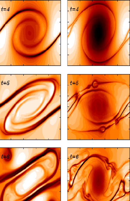
Figure 9: Evolution of the density at times $t=4$ (top), $t=5$ (middle), and $t=6$ (bottom), for the case of a uniform (left frames) and of a reversed field (right frames). We took $k_{x}=2\pi$, $V_{0}=0.645$, and $B_{0}=0.129$. The non-linear development differs markedly.

Figures 6, 7, and 8 show the dependence of the saturation level $E_{max}$ on the wavenumber, Alfvénic Mach number, and sound Mach number, respectively. Note how the saturation level for the hydrodynamic and the uniform MHD case monotonically increases with decreasing wavenumber in Fig. 6, while we demonstrated in Fig. 3 that the growth rate has a pronounced maximum in the range of wavenumbers considered. As a consequence, the linearly fastest growing mode does not necessarily correspond to the dominant mode in the non-linear evolution. However, the stabilizing effect of a uniform magnetic field persists in the non-linear regime (see [Frank et al. (1996)] and [Malagoli et al. (1996)]), as we find saturation levels which are always lower than in a pure HD case. Part of the available energy must be used to compress and stretch the field lines, leading to a lower $E_{max}$. For the reversed field case, no clear trend with wavenumber is apparent, and the KH instability can saturate at intermediate, lower or higher levels when compared to pure HD or uniform MHD cases. We point out that the reversed case is most susceptible to the inherent numerical diffusion. By calculating reversed cases on larger grids, and by investigating the limiting $\eta\rightarrow 0$ behaviour, we are confident that the observed variation is real. Nevertheless, the absolute values for the saturation level for the reversed field cases are less certain than the ones shown for hydrodynamic and uniform MHD cases. The saturation levels for the reversed case are fairly insensitive to the specific initial $B_{x}$ profile: the reference case with an initial discontinuity at $y=0$ saturated at $2E_{max}/\rho_{0}V_{0}^{2}\simeq 0.033$, while starting from a $\tanh(y/b)$ with $b=0.01$, the saturation was reached at $\simeq 0.039$. The qualitative non-linear behaviour is identical.

The dependence of the saturation level on Alfvénic Mach number at fixed $k_{x}=2\pi$ is shown in Fig. 7. The hydrodynamic saturation level is situated at $2E_{max}/\rho_{0}V_{0}^{2}\simeq 0.038$ (horizontal dotted line), and the uniform MHD case approaches this value from below when the initial field strength is decreased. However, the reversed case saturates sooner than the uniform MHD case at initial field strengths $B_{0}\geq 0.18$, while for $B_{0}\leq 0.1$, it saturates above the HD limit. Varying the shear flow $V_{0}$ at fixed wavenumber $k_{x}=2\pi$ as in Fig. 5 leads to a similarly complicated dependence of the saturation level on the sound Mach number $M_{s}$. Fig. 8 demonstrates how at this wavenumber and for fixed initial field strength $B_{0}=0.129$, both the uniform and the reversed MHD cases saturate at a lower level than a pure hydrodynamic situation.

To gain insight in the non-linear behaviour of the KH instability in both uniform and reversed MHD cases, we confront in Fig. 9 time series of the density pattern for both. We took the initial parameters as in the reference cases ($k_{x}=2\pi$, $V_{0}=0.645$ and $B_{0}=0.129$), but as our interest is now in the non-linear regime only, we took $v_{y0}=0.01$ so that the non-linear stage can be reached at a lower computational cost. The uniform case at left was calculated in ideal MHD on a $300\times 600$ grid, while the reversed case at right is done in resistive MHD with $\eta=10^{-5}$ and the use of $400\times 800$ grid points. We show the part of the grid between $-0.3\leq y\leq 0.3$. The contour levels differ from frame to frame, as we renormalized individual colour ranges by the instantaneous extremal values of the density to bring out all detail. The actual range of density values over all frames plotted is $0.58\leq\rho(x,y,t)\leq 1.15$.

The frames for the uniform MHD case are in good agreement with Malagoli et al. (1996). These authors concluded that the evolution of the KH instability in the presence of an initially uniform field consists of three phases. First, the instability grows exponentially, very much like Fig. 1. Second, the density pattern becomes completely controlled by the magnetic field which is strengthened in the process and becomes dynamically important. Indeed, field lines are pushed away from the center of the layer and stretched by the vortical flow. The first snapshot shown in Fig. 9 corresponds to the time of saturation where the dark lanes in the regions of enhanced density (bright) outline these stretched and compressed field lines. From the moment where the gradient scales across these field lines diminish to trigger (numerical) dissipation in this ideal MHD run, reconnection events occur. The second and third snapshot shows the density pattern in the first stages of this regime. At that point, the magnetic energy has already reached its maximum value, and starts to decay oscillatory. The third and final phase is one where small scale turbulence develops, until a new statistically-steady flow sets in. We have continued our calculation, and in agreement with [Malagoli et al. (1996)], we end up with an enlarged, mixed layer directed along the initial shear flow, aligned with the magnetic field (not shown).

The frames at right for the reversed case are dramatically different. We already mentioned that even in the linear regime, flux cancellation at $y=0$ sets in almost instantly. In fact, the reversed MHD case starts to resemble a pure HD case more closely: the top right panel ($t=4$) shows how a central density depletion (dark) forms since the dissipated field there no longer controls the dynamics. The effects of the magnetic field are most pronounced at some distance away from the initial interface at $y=0$, and at those regions where field lines are pushed together. Already at the first frame shown at $t=4$, an island structure is evident within the region of enhanced density (bright). In contrast to the uniform case, now anti-parallel field lines are pushed together there. Such a situation is tearing unstable in resistive MHD, and leads to the formation of a magnetic island, which influences the density dynamically to form the pattern shown. This process continues along the current sheet, as seen in the second frame where more, smaller islands are evident. Reconnection and tearing thus occurs all along the current sheet as it gets amplified by the KH vortical flow.

Naturally, the initially reversed field is thereby dissipated faster than in the uniform MHD case. A crude monitor for this is given by the time evolution of the total magnetic energy $E_{mag}(t)=\int\int\,\,dx\,dy(B_{x}^{2}+B_{y}^{2})/2$ for both cases. This is shown in Fig. 10 where the uniform case (dashed line) is compared to the reversed case (solid line). Note how the maximal magnetic energy reached in the reversed case is much lower than for a uniform background field of equal strength. The inset shows the result of a convergence study in resistive MHD for the reversed case only: fixing $\eta=10^{-5}$, we compare calculations on grids of size $150\times 300$, $300\times 600$ and $400\times 800$. The time evolution of the vertical kinetic energy $E_{y}(t)$, used to determine the saturation levels earlier, is clearly captured on all grids up to $t=5$. The magnetic field pattern at $t=5$ for the reversed case is shown in Fig. 11. The islands coincide with the density perturbations visible in Fig. 9 (middle right panel). Beyond this time, small-scale turbulence sets in. This is evident from the last panel (time $t=6$) shown in Fig. 9.

Figure 10: Evolution of the magnetic energy $E_{mag}(t)$ for the case of a uniform (dashed) and of a reversed field (solid). The uniform case is calculated in ideal MHD on a $300\times 600$ grid. The reversed case is a resistive MHD run with $400\times 800$ grid points. The inset shows the evolution of the vertical kinetic energy $E_{y}(t)$ for resistive $\eta=10^{-5}$ MHD runs on $150\times 300$, $300\times 600$ and $400\times 800$ grids.

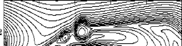
Figure 11: Island formation due to tearing instability for a reversed MHD case. We show the magnetic field structure at $t=5$, corresponding to the middle right frame of Fig. 9.

To demonstrate that the island formation correctly represents the non-linear development of combined current-vortex sheets (initial $\tanh$ profiles for both $v_{x}$ and $B_{x}$), we show in Fig. 12 the amplification of an initial continuous current sheet with $b=0.01$ by the developing vortex flow. All other parameters are as in the reference reversed case shown in Fig. 9, but now we took a $150\times 300$ grid with grid accumulation about $y=0$. The last frame shown corresponds with the top right panel of Fig. 9. The island structure is cospatial with the pronounced current maximum.

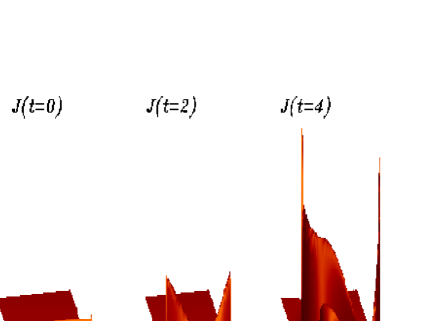
Figure 12: The amplification of an initially continuous current sheet in a KH unstable shear flow. Apart from the finite extent of the current sheet at $t=0$, parameters are identical to our reference reversed case shown at left in Fig. 9.

6 Discussion and conclusions

We studied the KH instability both in hydrodynamics and in magnetohydrodynamics with the Versatile Advection Code (VAC). We investigated the linear and the non-linear saturation regime by varying wavenumbers, sound Mach numbers, and, for the uniform and reversed field MHD case, the Alfvénic Mach number. While non-linear results for the hydrodynamic and uniform MHD cases confirm and extend results by previous authors, we demonstrated that novel physical effects appear when a reversed magnetic field is imposed.

The linear results clearly show the stabilizing effect of the uniform magnetic field, leading to smaller growth rates than the hydrodynamic case. This stabilizing effect is also present in the non-linear regime, since the strengthened, initially uniform field eventually halts the exponential growth sooner. This phase where the magnetic field controls the density pattern, eventually decays into a turbulent regime, as previously pointed out by [Malagoli et al. (1996)]. We focused on the saturation behaviour of the KH instability, and discussed its dependence on wavenumber and Mach numbers.

When the shear flow coincides with a field reversal, reconnection takes place right away, so our results for the reversed case are applicable in resistive MHD. We started from a situation where the field reversal is modeled as a discontinuity, seen as the limiting case of cospatial current-vortex sheets where the region of field reversal is completely contained within the region of velocity shear (see also [Dahlburg et al. (1997), Dahlburg (1998)]). In the linear regime, we find an overall larger growth rate than in hydrodynamic and uniform magnetohydrodynamic cases. Hence, a reversed field destabilizes the KH instability, and when the strength of the reversed magnetic field decreases, we approach the hydrodynamic growth rate from above. Comparisons with cases where the field reversal is a continuous $\tanh$-profile revealed that this linear destabilization is sensitive to the initial condition. Only for moderate magnetic fields (like our reference reversed case), the destabilizing effect persists when the region of magnetic shear is significantly narrower than the region of velocity shear. The role played by the initial pressure profile is crucial for stronger and wider current sheets. Such strongly magnetized, wide current sheets have been the subject of analytic studies of current-vortex sheets in incompressible MHD ([Dahlburg et al. (1997)]). There, the ratio of the magnetic shear width to the velocity shear width ($b/a$ in our terminology) was typically taken around unity and the Alfvén Mach number was varied from 0.6 to 1.2. We restricted our study to cases where $b\ll a$ and $M_{a}>1$, since it is known that the uniform MHD case is fully stabilized when $M_{a}=1$. Our study indicates (cfr. the evolution of the density in Fig. 9) that compressibility plays an important role in current-vortex sheet dynamics. We focused on KH unstable configurations where the magnetic effects are secondary. To make the connection with the results of [Dahlburg et al. (1997)] more explicit, we also calculated one case with $b=0.2a$ and $M_{a}=1$, setting $\eta=10^{-3}$, very much like Case I of their study. In our compressible simulation, the density varied locally up to 40 % during the development and the saturation of the then dominant tearing instability. A quantitative comparison with the incompressible simulations is therefore fairly complicated.

In our reversed case study, reconnection sets in almost instantly at the shear flow interface and the reconnected field lines act to enforce the KH instability. Flux cancellation at $y=0$ clearly alters the field structure earlier than in a similar field-strength uniform case. While the uniform magnetic field effectively prevented the build up of a central density perturbation, by dynamically influencing the flow pattern throughout the inner region, the field in the reversed case changes the flow and density most markedly at some distance away from $y=0$. Reconnection is also important in those regions where anti-parallel field lines are pushed together, thereby amplifying the initial current sheet. We showed how the KH flow may thus in turn drive this sheet unstable. Resistive tearing modes form magnetic islands and influence the density pattern by isolating blobs of enhanced density. Decay to a turbulent regime sets in sooner than for a uniform MHD case of equal field strength.

The temporal evolution of the total magnetic energy shows a much lower maximal energy level in the case of the reversed field compared to the uniform field case. The saturation as measured by the first maximum in the vertical kinetic energy indicates that the reversed field can saturate at a lower, a higher, or at an intermediate level between a pure hydrodynamic and a uniform MHD case. The temporal evolution of the density in the reversed field case initially resembles the hydrodynamic case more closely.

The plane-parallel configuration we investigated here is relatively simple, however, we expect that the basic features of the KH instability are well-described in our model. Meaningful extensions would model the evolution in three dimensions. A first step is found in [Miura (1997)], where a magnetic field in the plane perpendicular to the velocity gradient is considered. There, it was found that the vortex train formed by the KH instability is further susceptible to vortex pairing following the non-linear saturation. For fluid applications, the surface tension can not be ignored. For certain astrophysical situations, an accurate treatment of the KH instability must include the influence of viscosity, gravity, and relativistic flows.