CMB in Open Inflation

Abstract

The possibility to have an infinite open inflationary universe inside a bubble of a finite size is one of the most interesting realizations extensively discussed in the literature. The original idea was based on the theory of tunneling and bubble formation in the theories of a single scalar field. However, for a long time we did not have any consistent models of this type, so it was impossible to compare predictions of such models with the observational data on the CMB anisotropy. The first semi-realistic model of this type was proposed only very recently, in hep-ph/9807493. Here we present the results of our investigation of the scalar and tensor perturbation spectra and the resulting CMB anisotropy in such models. In all models which we have studied there are no supercurvature perturbations. The spectrum of scalar CMB anisotropies has a minimum at small  $\ell$ and a plateau at $\ell=O(10)$ for low $\Omega_{0}$. Meanwhile tensor CMB anisotropies are peaked at $\ell=2$. Relative magnitude of the scalar CMB spectra versus tensor CMB spectra at small $\ell$ depends on the parameters of the models.

]

I Introduction

Inflationary theory has a robust prediction: Our universe must be almost exactly flat, $\Omega_{0}=\Omega_{\rm matter}+\Omega_{\Lambda}=1\pm O(10^{-4})$. If this result is confirmed by observational data, we will have a decisive confirmation of inflationary cosmology. However, what if observational data show that the universe is open?

Until very recently, we did not have any consistent cosmological models, inflationary or not, describing a homogeneous open universe. An assumption that all parts of an infinite universe can be created simultaneously and have the same value of energy density everywhere did not have any justification. This problem was solved only after the invention of inflationary cosmology. It was found that each bubble of a new phase formed during the false vacuum decay in inflationary universe looks from inside like an infinite open universe [1, 2]. The process of bubble formation in the false vacuum is described by the Coleman-De Luccia (CDL) instantons [1]. If this universe continues inflating inside the bubble, then we obtain an open inflationary universe. Then by a certain fine-tuning of parameters one can get any value of $\Omega_{0}$ in the range $0<\Omega_{0}<1$ [3, 4].

Even though the basic idea of this scenario was pretty simple, it was very difficult to find a realistic open inflation model. The general scenario proposed in [3, 4] was based on investigation of chaotic inflation and tunneling in the theories of a single scalar field $\phi$. However, no models where this scenario could be successfully realized have been proposed so far. As it was shown in [5], in the simplest models with polynomial potentials of the type of ${m^{2}\over 2}\phi^{2}-{\delta\over 3}\phi^{3}+{\lambda\over 4}\phi^{4}$ the tunneling occurs not by bubble formation, but by jumping onto the top of the potential barrier described by the Hawking-Moss instanton [6]. This process leads to formation of inhomogeneous domains of a new phase, and the whole scenario fails. The main reason for this failure is rather generic [7]. Typically, CDL instantons exist only if $|\partial^{2}V|>H^{2}$ during the tunneling (here and in the rest of the paper $\partial^{2}V$ stays for $\partial^{2}V/\partial\phi^{2}$). Meanwhile, inflation, which, according to [3, 4], begins immediately after the tunneling, typically requires $|\partial^{2}V|\ll H^{2}$. These two conditions are almost incompatible.

This problem can be avoided in models of two scalar fields [5]. However, in this paper we will concentrate on the one-field open inflation. We will remember why it was so difficult to realize this scenario. Then we will describe two models where this can be accomplished; one of these models was proposed recently in [7]. The main purpose of this paper is to investigate the CMB anisotropy in these models. As we will see, CMB anisotropy in these models has some distinguishing features, which may serve as a signature for the one-filed open inflation models.

II Toy models of one-field open inflation

To explain the main features of the one-field open inflation models, let us consider an effective potential $V(\phi)$ with a local minimum at $\phi_{0}$, and a global minimum at $\phi=0$, where $V=0$. In an $O(4)$-invariant Euclidean spacetime with the metric

$$ds^{2}=d\tau^{2}+a^{2}(\tau)(d\chi_{E}^{2}+\sin^{2}\chi_{E}\,d\Omega_{2}^{2})\ ,$$ (1)

the scalar field $\phi$ and the three-sphere radius $a$ obey the equations of motion

$$\ddot{\phi}+3{\dot{a}\over a}\dot{\phi}=\partial V\ ,~{}~{}~{}\ddot{a}=-{8\pi\over 3}a(\dot{\phi}^{2}+V)\ ,$$ (2)

where dots denote derivatives with respect to $\tau$. Here and in what follows we will use the units where $M_{p}=G^{-1/2}=1$.

An instanton which describes the creation of an open universe was first found by Coleman and De Luccia [1]. It is given by a slightly distorted de Sitter four-sphere of radius $H^{-1}(\phi_{0})$, with $a\approx H^{-1}\sin H\tau$. The field $\phi$ lies on the ‘true vacuum’ side of the maximum of $V$ in a region near $\tau=0$, and it is very close to the false vacuum, $\phi_{0}$, in the opposite part of the four-sphere near $\tau_{i}\approx\pi/H$, The scale factor $a(\tau)$ vanishes at the points $\tau=0$ and $\tau=\tau_{\rm i}$. In order to get a singularity-free solution, one must have $\dot{\phi}=0$ and $\dot{a}=\pm 1$ at $\tau=0$ and $\tau=\tau_{\rm i}$. This configuration interpolates between some initial point $\phi_{i}\approx\phi_{0}$ and the final point $\phi_{f}$. After an analytic continuation to the Lorentzian regime, it describes an expanding bubble which contains an open universe [1].

Solutions of this type can exist only if the bubble can fit into de Sitter sphere of radius $H^{-1}(\phi_{0})$. To understand whether this can happen, remember that at small $\tau$ one has $a\sim\tau$, and Eq. (2) coincides with equation describing creation of a bubble in Minkowski space, with $\tau$ being replaced by the bubble radius $r$:  $\ddot{\phi}+{3\over r}\dot{\phi}=\partial V$ [8]. Here the radius of the bubble can run from $0$ to $\infty$. Typically the bubbles have size greater than the Compton wavelength of the scalar field, $r\gtrsim m^{-1}\sim(\partial^{2}V)^{-1/2}$ [9].

In de Sitter space $\tau$ cannot be greater than ${\pi\over H}$, and in fact the main part of the evolution of the field $\phi$ must end at $\tau\sim{\pi\over 2H}$. Indeed, once the scale factor reaches its maximum at $\tau\sim{\pi\over 2H}$, the coefficient ${\dot{a}\over a}$ in Eq. (2) becomes negative, which corresponds to anti-friction. Therefore if the field $\phi$ still changes rapidly at $\tau>{\pi\over 2H}$, it experiences ever growing acceleration near $\tau_{\rm f}$, and typically the solution becomes singular [10]. Thus the Coleman-De Luccia (CDL) instantons exist only if ${\pi\over 2H}>(\partial^{2}V)^{-1/2}$, i.e. if $\partial^{2}V>H^{2}$. This condition must be satisfied at small $\tau$, which corresponds to the endpoint of the tunneling, where inflation should begin in accordance with the scenario of Ref. [3, 4]. But this condition is opposite to the standard inflationary condition $\partial^{2}V\ll H^{2}$.

This means that immediately after the tunneling the field begins rolling much faster than it was anticipated in [3, 4]. As a result, in many models, such as the models with the effective potential $V(\phi)={m^{2}\over 2}\phi^{2}-{\delta\over 3}\phi^{3}+{\lambda\over 4}\phi^{4}$, the open inflation scenario simply does not work [5, 7]. This problem is very general, and for a long time we did not have any model where this scenario could be realized. We will describe two of these models here, one of which was proposed recently in [7]. We do not know as yet whether it is possible to derive these models from some realistic theory of elementary particles, so for the moment we consider them simply as toy models of open inflation. Still we believe that these models deserve investigation because they share the generic property of all models of this class: As we expected. immediately after the tunneling one has $\partial^{2}V>H^{2}$. As we will see, this condition suppresses scalar perturbations of metric produced soon after the tunneling. The supercurvature perturbations are also suppressed, whereas the tensor perturbations in these models may be quite strong. These features may help us to distinguish one-field models of open inflation based on the Coleman-De Luccia tunneling from other models of open inflation.

The first model which we are going to consider has the effective potential of the following type:

$$V(\phi)={m^{2}\phi^{2}\over 2}\left(1+{\alpha^{2}\over\beta^{2}+(\phi-v)^{2}}\right).$$ (3)

Here $\alpha$ $\beta$ and $v$ are some constants; we will assume that $\beta\ll v$. The first term in this equation is the potential of the simplest chaotic inflation model ${m^{2}\phi^{2}\over 2}$. The second term represents a peak of width $\beta$ with a maximum near $\phi=v$. The relative hight of this peak with respect to the potential ${m^{2}\phi^{2}\over 2}$ is determined by the ratio ${\alpha^{2}\over\beta^{2}}$.

FIG. 1.: Effective potential our first model, see Eq. (3). All values are given in units where $M_{p}=1$.

As an example, we will consider the theory with $m=1.5\times 10^{-6}$, which is necessary to have a proper amplitude of density perturbations during inflation in our model. We will take $v=3.5$, which, as we will see, will provide about 65 e-folds of inflation after the tunneling. By changing this parameter by few percent one can get any value of $\Omega_{0}$ from $0$ to $1$. For definiteness, in this section we will take $\beta^{2}=2\alpha^{2}$, $\beta=0.1$. This is certainly not a unique choice; other values of these parameters to be considered in the next section can also lead to a successful open inflation scenario. The shape of the effective potential in this model is shown in Fig. 1.

As we see, this potential coincides with ${m^{2}\phi^{2}\over 2}$ everywhere except a small vicinity of the point $\phi=3.5$, but one cannot roll from $\phi>3.5$ to $\phi<3.5$ without tunneling through a sharp barrier. We have solved Eq. (2) for this model numerically and found that the Coleman-De Luccia instanton in this model does exist. It is shown in Fig. 2.

FIG. 2.: Coleman-De Luccia instanton in the first model. The upper panel shows the function $\phi(\tau)$, the lower panel demonstrates that most of the time during the tunneling one has $|\partial^{2}V|\gg H^{2}$.

The upper panel of Fig. 2 shows the CDL instanton $\phi(\tau)$. Tunneling occurs from $\phi_{i}\approx 3.6$ to $\phi_{f}\approx 3.4$. The energy density decreases in this process, $V(\phi_{f})<V(\phi_{i})$. The lower panel of Fig. 2 shows the ratio $\partial^{2}V/H^{2}$. Almost everywhere along the instanton trajectory $\phi(\tau)$ one has $|\partial^{2}V|>H^{2}$. That is exactly what we have expected on basis of our general arguments concerning CDL instantons.

An interesting feature of the CDL instantons is that the evolution of the field $\phi$ does not begin exactly at the local minimum of the effective potential. This is similar to what happens in the Hawking-Moss case [6], where tunneling begins and ends not at the local minimum but at the top of the effective potential; see [11] for a recent discussion of this issue. This unconventional feature of the CDL instantons was not emphasized in [1] because the authors concentrated on the thin wall approximation where this effect disappears. For a proper interpretation of these instantons, just as in the Hawking-Moss case, one may either glue to the point $\tau_{f}$ a de Sitter hemisphere corresponding to the local minimum of the effective potential [11], or use a construction proposed in [12]. It would be very desirable to verify the Coleman-De Luccia approach by a complete Hamiltonian analysis of the tunneling in inflationary universe.

The second model has the effective potential of the following type:

$$V(\phi)={m^{2}\over 2}\left(\phi^{2}+B^{2}{\sinh A(\phi-v)\over\cosh^{2}A(\phi-v)}\right)$$ (4)

Here $A$, $B$ and $v$ are some constants. As an example, we will consider the theory with $m=1.0\times 10^{-6}$, $v=3.5$, $A=20$, and $B=4$. The shape of the effective potential in this model is shown in Fig. 3.

FIG. 3.: Effective potential in our second model, Eq. (4). All values are given in units where $M_{p}=1$.

The Coleman-De Luccia instanton in this model is shown in Fig. 4. The upper panel of Fig. 4 shows the instanton $\phi(\tau)$. Tunneling occurs from $\phi_{i}\approx 3.54$, which almost exactly coincides with the position of the local minimum of $V(\phi)$, to $\phi_{f}\approx 3.30$. The energy density increases in this process, $V(\phi_{f})>V(\phi_{i})$. This may seem unphysical, but in fact such jumps are possible because of the gravitational effects. A similar effect occurs during the Hawking-Moss tunneling to the local maximum of the effective potential [6]. The lower panel of Fig. 4 shows that almost everywhere along the trajectory $\phi(\tau)$ one has $|\partial^{2}V|\gg H^{2}$. After the tunneling the scalar field slowly rolls down and then oscillates near the minimum of the effective potential at $\phi=0$. During the stage of the slow rolling, the scale factor in the models which we investigated expands approximately $e^{65}$ times.

FIG. 4.: Coleman-De Luccia instanton in our second model. The upper panel shows the function $\phi(\tau)$, the second one shows the ratio $|\partial^{2}V|/H^{2}$, which remains very large during the tunneling.

III CMB anisotropy in the open inflation models

Just as we expected, in both models the tunneling brings the field to the region where $|\partial^{2}V|>H^{2}$. Therefore the usual scalar perturbations of density are not produced in these models immediately after the open universe formation. As we will see now, this leads to a suppression of the contribution of these perturbations to the CMB anisotropy at $\ell\lesssim 10$.

In addition to these perturbations, we could encounter supercurvature perturbations which are produced in the false vacuum outside the bubble and may later penetrate into its interior during the bubble expansion. However, we did not find any supercurvature perturbations in these models.

The reason why there are no supercurvature perturbations in the second model is pretty simple: The curvature of the effective potential in the false vacuum is much greater than $H^{2}$, so these perturbations are not produced outside the bubble.

For the first model the reason for the absence of the supercurvature modes is less obvious because in the false vacuum there one has $\partial^{2}V\ll H^{2}$. However, all information about the interior of the bubble can be obtained by the analytical continuation of the CDL instanton, which begins away from the false vacuum, in a state with $\partial^{2}V>H^{2}$. The fact that there is no region where $\partial^{2}V\ll H^{2}$ in the CDL instanton implies that the initial distance from the center of the bubble to the place where $\partial^{2}V$ becomes smaller than $H^{2}$ (in the false vacuum outside of the CDL instanton) is greater than $2H^{-1}$, i.e., it is greater than twice the size of the event horizon in de Sitter space. As a result, the fluctuations produced in the false vacuum do not penetrate into the bubble.

In addition to the scalar perturbations, there also exist tensor perturbations. Unlike the standard inflation scenario, it is known that the fluctuations of the bubble wall contribute to the low frequency spectrum of tensor perturbations and the contribution can dominate over the scalar spectrum [13, 14]. In fact, we shall see that they can be quite significant and dominate the CMB anisotropy spectrum for small $l$.

Below we present the scalar and tensor spectra for three models: Two of them are those discussed in the previous section. The third model is the one with the same potential form as the first model but with a different value of $\beta$; $\beta^{2}=\alpha^{2}/2=0.0025$. To compute the spectra, we adopt a gauge-invariant method developed by Garriga, Montes, Sasaki and Tanaka [15, 16]. Then we show the resulting CMB anisotropy spectra on large angular scales.

A Scalar and tensor perturbation spectra

Let us first summarize the procedure to obtain the scalar and tensor spectra. The metric describing the Lorentzian bubble configuration is given by the analytic continuation of (1) with $\chi_{E}=-i\chi_{C}+\pi/2$:

$$ds^{2}=d\tau^{2}+a^{2}(\tau)(-d\chi_{C}^{2}+\cosh^{2}\chi_{C}\,d\Omega_{2}^{2})\,.$$ (5)

The scalar field configuration is still given by $\phi=\phi(\tau)$. In the one-field models of one-bubble open inflation, the scalar perturbation is conveniently described by a variable $\textstyle q$, which is essentially equivalent to the gravitational potential perturbation $\Psi_{N}$ in the Newton gauge,

$$\mathchoice{{\hbox{\boldmath$\displaystyle q$}}}{{\hbox{\boldmath$\textstyle q$}}}{{\hbox{\boldmath$\scriptstyle q$}}}{{\hbox{\boldmath$\scriptscriptstyle q$}}}={\Psi_{N}\over 4\pi G\dot{\phi}}\,.$$ (6)

Here and below we recover $G$ in equations. The (even parity) tensor perturbation is described by a variable $\textstyle w$, whose relation to the transverse-traceless metric perturbation in the open universe will be given later. There are also odd parity modes for the tensor perturbation. But since the odd parity modes do not contribute to the CMB anisotropy, we shall not discuss them. Here we just mention that the form of the Lagrangians for both $\textstyle q$ and $\textstyle w$ is that for a scalar field with $\tau$-dependent mass [15, 16].

We quantize the variables $\textstyle q$ and $\textstyle w$ on the $\chi_{C}={\rm const.}$ hypersurface which is a Cauchy surface and which contains all the information of the bubble configuration. We expand them in terms of the spherical harmonics $Y_{\ell m}$ and spatial eigenfunctions $\mathchoice{{\hbox{\boldmath$\displaystyle q$}}}{{\hbox{\boldmath$\textstyle q$}}}{{\hbox{\boldmath$\scriptstyle q$}}}{{\hbox{\boldmath$\scriptscriptstyle q$}}}^{p}$ and $\mathchoice{{\hbox{\boldmath$\displaystyle w$}}}{{\hbox{\boldmath$\textstyle w$}}}{{\hbox{\boldmath$\scriptstyle w$}}}{{\hbox{\boldmath$\scriptscriptstyle w$}}}^{p}$ with eigenvalue $p^{2}$:

$$q = \sum\hat{a}_{p\ell m}f^{p\ell}(\chi_{C})\mathchoice{{\hbox{\boldmath$\displaystyle q$}}}{{\hbox{\boldmath$\textstyle q$}}}{{\hbox{\boldmath$\scriptstyle q$}}}{{\hbox{\boldmath$\scriptscriptstyle q$}}}^{p}(\tau)Y_{\ell m}(\Omega_{2})+{\rm h.c.}\,,$$ (7)

$$w = \sum\hat{b}_{p\ell m}f^{p\ell}(\chi_{C})\mathchoice{{\hbox{\boldmath$\displaystyle w$}}}{{\hbox{\boldmath$\textstyle w$}}}{{\hbox{\boldmath$\scriptstyle w$}}}{{\hbox{\boldmath$\scriptscriptstyle w$}}}^{p}(\tau)Y_{\ell m}(\Omega_{2})+{\rm h.c.}\,,$$ (8)

where $\hat{a}_{p\ell m}$ and $\hat{b}_{p\ell m}$ are the annihilation operators. The spatial eigenfunctions $\mathchoice{{\hbox{\boldmath$\displaystyle q$}}}{{\hbox{\boldmath$\textstyle q$}}}{{\hbox{\boldmath$\scriptstyle q$}}}{{\hbox{\boldmath$\scriptscriptstyle q$}}}^{p}$ and $\mathchoice{{\hbox{\boldmath$\displaystyle w$}}}{{\hbox{\boldmath$\textstyle w$}}}{{\hbox{\boldmath$\scriptstyle w$}}}{{\hbox{\boldmath$\scriptscriptstyle w$}}}^{p}$ satisfy, respectively,

$$\left[-{d^{2}\over d\eta_{C}^{2}}+U_{S}(\eta_{C})\right]{\mathchoice{{\hbox{\boldmath$\displaystyle q$}}}{{\hbox{\boldmath$\textstyle q$}}}{{\hbox{\boldmath$\scriptstyle q$}}}{{\hbox{\boldmath$\scriptscriptstyle q$}}}}^{p} =p^{2}{\mathchoice{{\hbox{\boldmath$\displaystyle q$}}}{{\hbox{\boldmath$\textstyle q$}}}{{\hbox{\boldmath$\scriptstyle q$}}}{{\hbox{\boldmath$\scriptscriptstyle q$}}}}^{p}\,;$$ (9)

$$U_{S}= {4\pi}G{\phi^{\prime}}^{2}+\phi^{\prime}\left({1\over\phi^{\prime}}\right)^{\prime\prime}-4\,,$$ (10)

$$\left[-{d^{2}\over d\eta_{C}^{2}}+U_{T}(\eta_{C})\right]{\mathchoice{{\hbox{\boldmath$\displaystyle w$}}}{{\hbox{\boldmath$\textstyle w$}}}{{\hbox{\boldmath$\scriptstyle w$}}}{{\hbox{\boldmath$\scriptscriptstyle w$}}}}^{p} =p^{2}{\mathchoice{{\hbox{\boldmath$\displaystyle w$}}}{{\hbox{\boldmath$\textstyle w$}}}{{\hbox{\boldmath$\scriptstyle w$}}}{{\hbox{\boldmath$\scriptscriptstyle w$}}}}^{p}\,;$$ (11)

$$U_{T}= {4\pi}G{\phi^{\prime}}^{2}\,,$$ (12)

where $d\eta_{C}=d\tau/a(\tau)$ and primes denote derivatives with respect to $\eta_{C}$. The potentials $U_{S}$ and $U_{T}$ both vanish for $\eta_{C}\to\pm\infty$, but $U_{S}$ is not necessarily positive definite. It then follows that if there exists a bound state for this eigenvalue equation, it exists discretely at some $p^{2}<0$ and corresponds to a supercurvature mode of the scalar spectrum. On the other hand, $U_{T}$ is manifestly positive definite and there is no supercurvature mode in the tensor spectrum. For both scalar and tensor perturbations, the spectrum is continuous for $p^{2}>0$. As noted before, we found no supercurvature mode in all of the three models.

The equation for $f^{p\ell}$ turns out to be model-independent and is given by

$$\left[-{1\over\cosh^{2}\chi_{C}}{\partial\over\partial\chi_{C}}\cosh^{2}\chi_{C}{\partial\over\partial\chi_{C}}-{\ell(\ell+1)\over\cosh^{2}\chi_{C}}\right]f^{p\ell}$$ (13)

$$\qquad=(p^{2}+1)f^{p\ell}.$$ (14)

In accordance with the Euclidean approach to the tunneling, we take the quantum states of $\textstyle q$ and $\textstyle w$ to be the Euclidean vacua. This implies that the positive frequency function $f^{p\ell}$ is regular at $\chi_{E}=\pi/2$ ($\chi_{C}=0$). Apart from the normalization, the solution is

$$f^{p\ell}(\chi_{C})\propto{1\over\sqrt{\cosh\chi_{C}}}P^{-\ell-1/2}_{ip-1/2}(i\sinh\chi_{C}),$$ (15)

where $P^{\mu}_{\nu}$ is the associated Legendre function of the first kind. The normalizations of the mode functions $f^{p\ell}\mathchoice{{\hbox{\boldmath$\displaystyle q$}}}{{\hbox{\boldmath$\textstyle q$}}}{{\hbox{\boldmath$\scriptstyle q$}}}{{\hbox{\boldmath$\scriptscriptstyle q$}}}^{p}$ and $f^{p\ell}\mathchoice{{\hbox{\boldmath$\displaystyle w$}}}{{\hbox{\boldmath$\textstyle w$}}}{{\hbox{\boldmath$\scriptstyle w$}}}{{\hbox{\boldmath$\scriptscriptstyle w$}}}^{p}$ are determined by the standard Klein-Gordon normalization of a scalar field.

We then analytically continue $\textstyle q$ and $\textstyle w$ to the region just inside the lightcone emanating from the center of the bubble, i.e., to the region of the open universe, by $\chi=\chi_{C}+i\pi/2$ and $t=-i\tau$ (or $\eta=\eta_{C}-i\pi/2$). The metric there is given by

$$ds^{2} = -dt^{2}+a^{2}(t)(d\chi^{2}+\sinh^{2}\chi\,d\Omega_{2}^{2})$$ (16)

$$= a^{2}(\eta)(-d\eta^{2}+d\chi^{2}+\sinh^{2}\chi\,d\Omega_{2}^{2})\,.$$ (17)

Then the function $f^{p\ell}$ just becomes the radial function of a spatial harmonic function on a unit spatial 3-hyperboloid,

$$\left(\mathop{\Delta}^{(3)}+p^{2}+1\right)Y^{p\ell m}=0\,;\quad Y^{p\ell m}=f^{p\ell}(\chi)Y_{\ell m}(\Omega_{2}).$$ (18)

On the other hand, the spatial eigenfunctions $\mathchoice{{\hbox{\boldmath$\displaystyle q$}}}{{\hbox{\boldmath$\textstyle q$}}}{{\hbox{\boldmath$\scriptstyle q$}}}{{\hbox{\boldmath$\scriptscriptstyle q$}}}^{p}$ and $\mathchoice{{\hbox{\boldmath$\displaystyle w$}}}{{\hbox{\boldmath$\textstyle w$}}}{{\hbox{\boldmath$\scriptstyle w$}}}{{\hbox{\boldmath$\scriptscriptstyle w$}}}^{p}$ become the temporal mode functions for the scalar and tensor perturbations, respectively, in the open universe. Note that $p\sim 1$ corresponds to the comoving spatial curvature scale. The evolution equations for $\mathchoice{{\hbox{\boldmath$\displaystyle q$}}}{{\hbox{\boldmath$\textstyle q$}}}{{\hbox{\boldmath$\scriptstyle q$}}}{{\hbox{\boldmath$\scriptscriptstyle q$}}}^{p}$ and $\mathchoice{{\hbox{\boldmath$\displaystyle w$}}}{{\hbox{\boldmath$\textstyle w$}}}{{\hbox{\boldmath$\scriptstyle w$}}}{{\hbox{\boldmath$\scriptscriptstyle w$}}}^{p}$ take the same forms as Eqs. (10) and (12), respectively, with the replacement $\eta_{C}\to\eta$. We solve Eqs. (10) and (12) until the scale of the perturbation is well outside the Hubble horizon scale, i.e., until

$$a^{2}H^{2}\gg p^{2}+1\,.$$ (19)

Here and in what follows, $H$ is not the inverse of the de Sitter radius but $H=\dot{a}/a$.

The important quantity that determines the primordial density perturbation spectrum as well as the large angle scalar CMB anisotropies is the curvature perturbation on the comoving hypersurface, ${\cal R}_{c}$. The comoving hypersurface is the one on which the scalar field fluctuation $\delta\phi$ vanishes. It is related to $\textstyle q$ as

$${\cal R}_{c}^{p}=-{4\pi G\dot{\phi}\,\mathchoice{{\hbox{\boldmath$\displaystyle q$}}}{{\hbox{\boldmath$\textstyle q$}}}{{\hbox{\boldmath$\scriptstyle q$}}}{{\hbox{\boldmath$\scriptscriptstyle q$}}}^{p}}+{H\over a\,\dot{\phi}^{2}}{d\over dt}\left(a\,\dot{\phi}\,\mathchoice{{\hbox{\boldmath$\displaystyle q$}}}{{\hbox{\boldmath$\textstyle q$}}}{{\hbox{\boldmath$\scriptstyle q$}}}{{\hbox{\boldmath$\scriptscriptstyle q$}}}^{p}\right).$$ (20)

Just as in the case of the flat universe inflation, ${\cal R}_{c}$ remains constant in time until the perturbation scale re-enters the Hubble horizon [17].

On the other hand, the even parity tensor perturbation in the open universe is described as

$$\delta g_{ij}=a^{2}t_{ij}\,;\quad t_{ij}=\sum\hat{b}_{p\ell m}U_{p}(\eta)Y^{(+)p\ell m}_{ij}+\hbox{h.c.}\,,$$ (21)

where $Y^{(+)p\ell m}_{ij}$ are the even parity tensor harmonics on the unit 3-hyperboloid [18]. After an appropriate choice of the normalization factor, $U_{p}$ is given in terms of $\mathchoice{{\hbox{\boldmath$\displaystyle w$}}}{{\hbox{\boldmath$\textstyle w$}}}{{\hbox{\boldmath$\scriptstyle w$}}}{{\hbox{\boldmath$\scriptscriptstyle w$}}}^{p}$ as [16]

$$U_{p}=-{8\pi G\over a\,(p^{2}+1)}{d\over dt}\,(a\,\mathchoice{{\hbox{\boldmath$\displaystyle w$}}}{{\hbox{\boldmath$\textstyle w$}}}{{\hbox{\boldmath$\scriptstyle w$}}}{{\hbox{\boldmath$\scriptscriptstyle w$}}}^{p}).$$ (22)

Similar to the case of the scalar perturbation, $U_{p}$ is known to remain constant in time on superhorizon scales.

In Fig. 5, the scalar and tensor perturbation spectra for the first, second and third models (which we call Models 1, 2 and 3, respectively) are shown. Let us recall their model parameters:

Model 1: $$\hbox{Eq.~{}(\ref{toy}) with}~{}\alpha^{2}=0.005,~{}\beta^{2}=2\alpha^{2},$$

$$\quad v=3.5,~{}m=1.5\times 10^{-6}.$$

Model 2: $$\hbox{Eq.~{}(\ref{toy2}) with}~{}A=20,~{}B=4,$$

$$\quad v=3.5,~{}m=1.0\times 10^{-6}.$$

Model 3: $$\hbox{Eq.~{}(\ref{toy}) with}~{}\alpha^{2}=0.005,~{}\beta^{2}=\alpha^{2}/2,$$

$$\quad v=3.5,~{}m=1.5\times 10^{-6}.$$

FIG. 5.: The spectra of scalar and tensor perturbations (per logarithmic interval of $p$) for Models 1, 2 and 3. The three curves that gradually increase as $p$ are the scalar spectra, and the other three that level off at large $p$ are the tensor spectra. The spectra for Models 1, 2 and 3 are shown by the solid, dot-dashed and dotted curves, respectively.

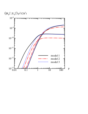
First let us consider the scalar spectra. As mentioned previously, there are no supercurvature modes in the present models. So the scalar perturbations are completely described by the continuous spectra shown in Fig 5. As seen from the figure, the scalar spectra for the three models are all alike: On the low frequency end, they decrease sharply as $p$ decreases, while they gradually increase for $p\gtrsim 10$. As discussed in the previous section, one can interpret this feature as due to the common evolutionary behavior of any successful one-field model with the CDL tunneling. The scalar field evolves rapidly for the first few expansion times when $\partial^{2}V>H^{2}$ and eventually decelerates as the slope of the effective potential becomes flatter. For $p\gg 1$, the spectrum approaches the one given by the standard formula for the flat universe inflation models. As shown in [7], the gradual increase gives rise to a peak in the spectrum at $p\sim 10^{4}$, which may have significant implications to the structure formation in the universe.

To understand the shape of the scalar spectrum more quantitatively, it is useful to compare the computed spectrum with the following analytic formula [17, 16],

$$|{\cal R}_{c}^{p}|^{2}{p^{3}\over 2\pi^{2}}=\left({H^{2}\over 2\pi\dot{\phi}}\right)^{2}_{t=t_{p}}{\cosh\pi p+\cos\delta_{p}\over\sinh\pi p}{p^{2}\over 1+p^{2}}\,,$$ (23)

where $t_{p}$ is an epoch slightly after the perturbation scale goes out of the Hubble horizon. This formula assumes $\partial^{2}V\ll H^{2}$ and the slow time variation of $\partial^{2}V$. The angle $\delta_{p}$ describes the effect of the bubble wall, which is known to behave as $\delta_{p}-\pi\propto p$ for $p\to 0$. The low frequency part of the spectrum is most suppressed when $\delta_{p}=\pi$. This case corresponds to the case when $\partial^{2}V\gg H^{2}$ on the false vacuum side of the instanton [17].

In our case the condition $\partial^{2}V\ll H^{2}$ is violated at the first stages after the bubble formation. Therefore Eq. (23) should be somewhat modified for small $p$. Indeed, fluctuations with small $p$ are produced soon after the tunneling. But immediately after the tunneling one has $\partial^{2}V>H^{2}$ in all models where the Coleman-De Luccia instantons exist. Therefore the perturbations with the wavelength greater than $H^{-1}$ will not become “frozen” immediately after the tunneling. They will freeze somewhat later, when the field $\phi$ will roll to the area with $\partial^{2}V\ll H^{2}$. But at that time their wavelength increases and their amplitude becomes smaller. As a result, Eq. (23) provides a good description of the spectrum at large $p$, but at small $p$ the amplitude of perturbations will be somewhat smaller than that given by Eq. (23). This expectation is confirmed by the results of our numerical investigation.

FIG. 6.: Comparison of the scalar and tensor spectra of Model 1 with the ones given by analytic formulas (23) and (28), respectively. The upper and lower dotted lines show the scalar and tensor formulas, respectively. The solid lines that coincide with the upper and lower dotted lines for $p\gg 1$ are, respectively, the computed scalar and tensor spectra.

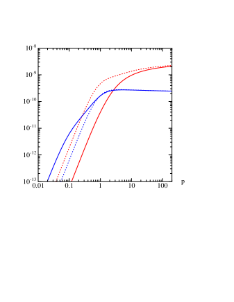
In Fig. 6, this comparison is made for Model 1. In the figure, the upper dotted line shows the formula (23) and the solid line that approaches it for $p\gg 1$ is the computed one. We choose $t_{p}$ to be the time when $a^{2}(2H^{2}-\partial^{2}V)=2(1+p^{2})$ and $\delta_{p}=\pi$. As one can see, the computed spectrum at small $p$ is significantly more suppressed than the most suppressed case of the analytic formula. As we shall see below, this large suppression relative to the analytic formula causes a large suppression of the CMB anisotropy at small $\ell$. The suppression of scalar perturbations with small $p$ and $\ell$ and the absence of supercurvature perturbations seem to be a generic property of the models of one-field open inflation based on the CDL tunneling. On the other hand, the spectrum become almost indistinguishable from the one given by Eq. (23) for $p\gg 1$. Thus the tilt of the spectrum (with a positive power-law index) is due to the slowing down of the evolution of $\phi$.

Now let us consider the tensor spectra. The spectra for Models 1 and 3 are indistinguishable at $p\gtrsim 1$, while the spectrum for Model 2 is about a factor of 2 smaller. This difference is due to the difference in the choice of the mass parameter: The mass square for Models 1 and 3 is $1.5^{2}=2.25$ greater than that for Model 2. This results in the difference in $H^{2}$. In fact, if we multiply the spectrum of Model 2 by 2.25, it becomes almost indistinguishable from the spectrum of Model 3 for the whole range of $p$. Turning to the low frequency behavior, the spectrum of Model 1 at $p\lesssim 1$ differs considerably from that of Model 3: The former is larger by an order of magnitude relative to the latter at small $p$. This enhancement is due to the wall fluctuation modes. Recall that the parameter $\beta$ for Model 1 is larger than that for Model 3. Since a larger $\beta$ means a lower potential barrier, the wall tension is smaller for Model 1 than for Model 3. This makes the wall of Model 1 easier to vibrate.

A non-dimensional quantity that represents the strength of the wall tension is given by the following integral over the instanton background [13]:

$$\Delta s=4\pi G\int\phi^{\prime}{}^{2}d\eta_{C}\,.$$ (24)

For Models 1, 2 and 3, the values of $\Delta s$ are found as

Model 1: $$\Delta s=0.1681\,,$$ (25)

Model 2: $$\Delta s=0.6614\,,$$ (26)

Model 3: $$\Delta s=0.6640\,.$$ (27)

In the thin-wall limit, $\Delta s=4\pi GR_{W}S_{1}$, where $R_{W}$ is the wall radius and $S_{1}$ is the surface tension. Further, in this limit, $\Delta s$ is always smaller than unity and the low frequency spectrum is enhanced by a factor $\sim 1/\Delta s^{2}$ for the width $\Delta p\sim\Delta s$ [13]. In the present case, as we have seen in section II, the bubble walls are not at all thin. Nevertheless, this qualitative feature expected from the thin-wall limit is in good agreement with the computed tensor spectra.

To see the effect of wall fluctuations more clearly, in Fig. 6, the tensor spectrum for Model 1 is compared with that given by the following approximate analytic formula derived in [19, 20, 15, 16]:

$$|U_{p}|^{2}{p^{3}\over 2\pi^{2}}=32\pi G\left({H\over 2\pi}\right)^{2}_{t=t_{p}}{\cosh\pi p-1\over\sinh\pi p}{p^{2}\over 1+p^{2}}\,,$$ (28)

where we took the large tension limit, which makes the wall fluctuations least effective. As seen from Fig. 6, the analytic formula agrees very well with the computed spectrum for $p\gtrsim 1$. Hence the difference at $p\lesssim 1$ is totally due to the wall fluctuation modes. If one compares the analytic tensor spectrum in Fig. 6 with the tensor spectrum of Model 3 in Fig. 5, one sees they almost coincide with each other. This is in accordance with the fact that $\Delta s$ of Model 3 is large, as shown in Eq. (25). Thus the bubble wall fluctuations are highly suppressed in Model 3 (and in Model 2) due to the large wall tension.

B Large angle CMB spectra

We now discuss the CMB anisotropies for Models 1, 2 and 3. We focus on the CMB anisotropy spectrum for $\ell\leq 20$. Since the contribution of scalar perturbations is dominated by the effect of gravitational potential perturbations, we take account of only the so-called Sach-Wolfe and integrated Sach-Wolfe effects. Although there is a possibility that $\Omega_{0}$ is dominated by $\Omega_{\Lambda}$, here we assume the present universe is matter-dominated; $\Omega_{0}=\Omega_{\rm matter}$.

Before going into discussion, we note one subtlety. In the one-bubble open universe scenario, the duration of inflation inside the bubble is directly related to the value of $\Omega_{0}$ today. In other words, once the model parameters are fixed, the duration of inflation is fixed and consequently so the value of $\Omega_{0}$. However, $\Omega_{0}$ depends rather sensitively on the values of the model parameters. In particular, it takes a very small change in $v$ to give a different $\Omega_{0}$. But such a change will not cause a change in the shape of perturbation spectra. Furthermore, the efficiency of reheating (or preheating) at the end of inflation will also affect the value of $\Omega_{0}$. So, depending on a grand scenario one has in mind, the resulting $\Omega_{0}$ will be different. Because of these reasons, below we present the CMB anisotropies of Models 1, 2 and 3 for several different values of $\Omega_{0}$ by artificially varying it.

The computed CMB spectra $\ell(\ell+1)C_{\ell}$ for Models 1, 2 and 3 are shown in Figs. 7, 8 and 9, respectively. The amplitudes shown there are the absolute amplitudes of the spectra for the given parameter values. It should be noted, however, that the amplitude can be tuned to fit the observed value (at certain $\ell$) by changing the value of $m$ if necessary. So, the important point is the relative amplitudes of the scalar and tensor contributions and their spectral shapes.

The scalar CMB anisotropies show similar spectral behavior for all the models. Namely, their amplitudes are suppressed at small $\ell$. This behavior is due to the large suppression of the scalar spectra at $p\lesssim 10$ mentioned in the previous subsection. If one compares the present results with the ones shown in Figs. 4, 5 and 6 of [4], one sees that the tendency is opposite: The scalar spectra obtained in [4] have a feature that they gradually decrease as $\ell$ increases. This is due to the integrated Sach-Wolfe effect and it is usually what one expects for open universe models. On the contrary, in the present case, because of the large suppression of the scalar spectra at $p\lesssim 10$, the corresponding CMB spectra increase for increasing $\ell$ and level off around $\ell\sim 10$.

FIG. 7.: The CMB spectra of Model 1 for several values of $\Omega_{0}$. The solid lines show the total CMB spectra. The dotted lines show the scalar contributions and the dot-dashed lines the tensor contributions. The values of $\Omega_{0}$ are 0.2, 0.4, 0.6 and 0.8 from top to bottom (at $\ell=3$) for each kind of curves.

FIG. 8.: The same as Fig. 7, but for Model 2.

FIG. 9.: The same as Fig. 7, but for Model 3.

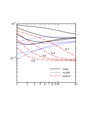
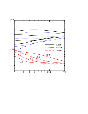
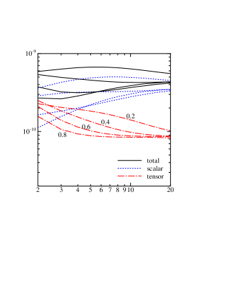
As expected from the tensor perturbation spectra shown in Fig. 5, the tensor CMB anisotropies at $\ell\lesssim 5-10$ are large in Model 1 due to large wall fluctuations, while they are small in Models 2 and 3. For Model 1, this enhancement causes a rise in the total spectra for $\ell\lesssim 5$, which does not seem to fit with the observed spectrum by COBE-DMR [21]. On the other hand, the tensor contribution to the CMB anisotropies of Models 2 and 3 is small. As a result, the total spectra of Models 2 and 3 turn out to be rather flat, which is consistent with the COBE spectrum.

IV Conclusions

Despite a lot of progress in our understanding of various versions of open inflation, until now we did not know how the spectrum of CMB may look in the simplest one-field open inflation models. Previous calculations have been based on the assumption that the usual inflationary perturbations are produced inside the bubble immediately after it is formed.

However, as we have argued (see also [7]), bubbles appear only if $\partial^{2}V>H^{2}$ at the moment of their formation in the one-field models. This means that the usual inflationary perturbations are not produced at that time.

In this paper we have studied the spectrum of CMB in several different models of one-field open inflation. At $\ell\gg 10$ the spectrum coincides with the spectrum obtained in the earlier papers on open inflation, since the mechanism of the bubble production is not very important for the behavior of the perturbations on scale much smaller than the size of the bubble. The main difference in the spectrum of CMB occurs at $\ell\lesssim O(10)$.

We have found that the spectrum of scalar CMB anisotropies has a minimum at small $\ell$, and reaches a plateau at $\ell=O(10)$. The existence of this minimum is a model-independent feature of the spectrum related to the fact that $\partial^{2}V>H^{2}$ at the moment of the bubble formation in the one-field models. In all models which we have studied there are no supercurvature perturbations. Tensor CMB anisotropies are peaked at $\ell=2$. Relative magnitude of the scalar CMB spectra versus tensor CMB spectra at small $\ell$ depends on the parameters of the models, and in particular on the value of $\Omega_{0}$. In some of the models, tensor perturbations are too large, which rules these models out. This effect is especially pronounced in the models with $\Omega_{0}\ll 1$. In some other models the tensor perturbations are very small even for $\Omega_{0}\ll 1$, and the combined spectrum of perturbations has a minimum at small $\ell$. In future satellite missions one could measure the tensor spectrum via polarization. This would make it possible to identify the scalar and tensor contributions to the CMB anisotropy [14] and to compare them with the predictions of the one-field models of open inflation. We conclude that the the spectrum of CMB in one-field models of open inflation has certain features which will help us to verify these models and to distinguish them from other versions of inflationary theory.

Acknowledgments

It is a pleasure to thank J. García–Bellido and R. Bousso for useful and stimulating discussions. The work of A.L. was supported in part by NSF grant PHY-9870115, and the work of M.S. and T.T. was supported in part by Monbusho Grant-in-Aid for Scientific Research No. 09640355.

REFERENCES

- [1] S. Coleman and F. De Luccia, Phys. Rev. D21, 3305 (1980).
- [2] J.R. Gott, Nature 295, 304 (1982); J.R. Gott, and T.S. Statler, Phys. Lett. 136B, 157 (1984).
- [3] M. Bucher, A.S. Goldhaber, and N. Turok, Phys. Rev. D52, 3314 (1995).
- [4] K. Yamamoto, M. Sasaki and T. Tanaka, Astrophys. J. 455, 412 (1995).
- [5] A.D. Linde, Phys. Lett. B351, 99 (1995); A.D. Linde and A. Mezhlumian, Phys. Rev. D 52, 6789 (1995).
- [6] S.W. Hawking and I.G. Moss, Phys. Lett. 110B, 35 (1982).
- [7] A.D. Linde, Phys. Rev. D59, 023503 (1999), hep-ph/9807493.
- [8] S. Coleman, Phys. Rev. D 15, 2929 (1977).
- [9] A.D. Linde, Nucl. Phys. B216, 421 (1983); Nucl. Phys. B372, 421 (1992).
- [10] S.W. Hawking and N. Turok, Phys. Lett. B425, 25 (1998), hep-th/9802030; S.W. Hawking and N. Turok, hep-th/9803156.
- [11] A.D. Linde, Phys. Rev. D 58, 083514 (1998), gr-qc/9802038,
- [12] R. Bousso and A. Chamblin, gr-qc/9803047.
- [13] M. Sasaki, T. Tanaka, and Y. Yakushige, Phys. Rev. D 56, 616 (1997).
- [14] J. García–Bellido, Phys. Rev. D 56, 3225 (1997), astro-ph/9702211.
- [15] J. Garriga, X. Montes, M. Sasaki and T. Tanaka, Nucl. Phys. B 513, 343 (1998).
- [16] J. Garriga, X. Montes, M. Sasaki and T. Tanaka, astro-ph/9811257.
- [17] K. Yamamoto, M. Sasaki and T. Tanaka, Phys. Rev. D 54, 5031 (1996).
- [18] K. Tomita, Prog. Theor. Phys. 68, 310 (1982).
- [19] T. Tanaka and M. Sasaki, Prog. Theor. Phys. 97, 243 (1997).
- [20] M. Bucher and J.D. Cohn, Phys. Rev. D 55, 7461 (1997).
- [21] G.F. Smoot et al., Astrophys. J. 396, L1 (1992); C.L. Bennett et al., Astrophys. J. 464, L1 (1996).