AN INTRODUCTION TO COSMOLOGICAL INFLATION

Abstract

An introductory account is given of the inflationary cosmology, which postulates a period of accelerated expansion during the Universe’s earliest stages. The historical motivation is briefly outlined, and the modelling of the inflationary epoch explained. The most important aspect of inflation is that it provides a possible model for the origin of structure in the Universe, and key results are reviewed, along with a discussion of the current observational situation and outlook.

1 Overview

One of the central planks of modern cosmology is the idea of inflation. Originally introduced by Guth [1] in order to explain the initial conditions for the hot big bang model, it has subsequently been given a much more important role as the currently-favoured candidate for the origin of structure in the Universe, such as galaxies, galaxy clusters and cosmic microwave background anisotropies. This article seeks to give an introductory account of the inflationary cosmology, with the focus aimed towards inflation as a model for the origin of structure.

It begins with a quick review of the big bang cosmology, and the problems with it which led to the introduction of inflation. The modelling of the inflationary epoch using scalar fields is described, and then results giving the form of perturbations produced by inflation are quoted. Finally, the current observational situation is briefly sketched.

2 Big bang problems and the idea of inflation

The standard hot big bang theory is an extremely successful one, passing some crucial observational tests of which I’d highlight five.

• The expansion of the Universe.

• The existence and spectrum of the cosmic microwave background radiation.

• The abundances of light elements in the Universe (nucleosynthesis).

• That the predicted age of the Universe is comparable to direct age measurements of objects within the Universe.

• That given the irregularities seen in the microwave background by COBE, there exists a reasonable explanation for the development of structure in the Universe, through gravitational collapse.

In combination, these are extremely compelling. However, the standard hot big bang theory is limited to those epochs where the Universe is cool enough that the underlying physical processes are well established and understood through terrestrial experiment. It does not attempt to address the state of the Universe at earlier, hotter, times. Furthermore, the hot big bang theory leaves a range of crucial questions unanswered, for it turns out that it can successfully proceed only if the initial conditions are very carefully chosen. The assumption of early Universe studies is that the mysteries of the conditions under which the big bang theory operates may be explained through the physics occurring in its distant, unexplored past. If so, accurate observations of the present state of the Universe may highlight the types of process occurring during these early stages, and perhaps even shed light on the nature of physical laws at energies which it would be inconceivable to explore by other means.

2.1 A hot big bang reminder

To get us started, I’ll give a quick review of the big bang cosmology. More detailed accounts can be found in any of a number of cosmological textbooks. One of my aims in this section is to set down the notation for the rest of the article.

2.2 Equations of motion

The hot big bang theory is based on the cosmological principle, which states that the Universe should look the same to all observers. That tells us that the Universe must be homogeneous and isotropic, which in turn tells us which metric must be used to describe it. It is the Robertson–Walker metric

$$ds^{2}=-dt^{2}+a^{2}(t)\left[\frac{dr^{2}}{1-kr^{2}}+r^{2}\left(d\theta^{2}+\sin^{2}\theta\,d\phi^{2}\right)\right]\,.$$ (1)

Here $t$ is the time variable, and $r$–$\theta$–$\phi$ are (polar) coordinates. The constant $k$ measures the spatial curvature, with $k$ negative, zero and positive corresponding to open, flat and closed Universes respectively. If $k$ is zero or negative, then the range of $r$ is from zero to infinity and the Universe is infinite, while if $k$ is positive then $r$ goes from zero to $1/\sqrt{k}$. Usually the coordinates are rescaled to make $k$ equal to $-1$, $0$ or $+1$. The quantity $a(t)$ is the scale-factor of the Universe, which measures its physical size. The form of $a(t)$ depends on the properties of the material within the Universe, as we’ll see.

If no external forces are acting, then a particle at rest at a given set of coordinates $(r,\theta,\phi)$ will remain there. Such coordinates are said to be comoving with the expansion. One swaps between physical (ie actual) and comoving distances via

$$\mbox{physical distance}=a(t)\times\mbox{comoving distance}\,.$$ (2)

The expansion of the Universe is governed by the properties of material within it. This can be specified  by the energy density $\rho(t)$ and the pressure $p(t)$. These are often related by an equation of state, which gives $p$ as a function of $\rho$; the classic examples are

$$p = \frac{\rho}{3}\quad\quad\mbox{Radiation}\,,$$ (3)

$$p = 0\quad\quad\;\;\mbox{Non-relativistic matter}\,.$$ (4)

In general though there need not be a simple equation of state; for example there may be more than one type of material, such as a combination of radiation and non-relativistic matter, and certain types of material, such as a scalar field (a type of material we’ll encounter later which is crucial for modelling inflation), cannot be described by an equation of state at all.

The crucial equations describing the expansion of the Universe are

$$H^{2}=\frac{8\pi}{3m_{{\rm Pl}}^{2}}\,\rho-\frac{k}{a^{2}}\quad\quad$$ Friedmann equation (5)

$$\dot{\rho}+3H(\rho+p)=0\quad\quad$$ Fluid equation (6)

where overdots are time derivatives and $H=\dot{a}/a$ is the Hubble parameter. The terms in the fluid equation contributing to $\dot{\rho}$ have a simple interpretation; the term $3H\rho$ is the reduction in density due to the increase in volume, and the term $3Hp$ is the reduction in energy caused by the thermodynamic work done by the pressure when this expansion occurs.

These can also be combined to form a new equation

$$\frac{\ddot{a}}{a}=-\frac{4\pi}{3m_{{\rm Pl}}^{2}}\left(\rho+3p\right)\quad\quad\mbox{Acceleration equation}$$ (7)

in which $k$ does not appear explicitly.

2.3 Standard cosmological solutions

When $k=0$ the Friedmann and fluid equations can readily be solved for the equations of state given earlier, leading to the classic cosmological solutions

$$\mbox{Matter Domination~{}~{}~{}~{}~{}~{}}p=0: \rho\propto a^{-3}\quad\quad a(t)\propto t^{2/3}$$ (8)

$$\mbox{Radiation Domination~{}~{}~{}~{}~{}~{}}p=\rho/3: \rho\propto a^{-4}\quad\quad a(t)\propto t^{1/2}$$ (9)

In both cases the density falls as $t^{-2}$. When $k=0$ we have the freedom to rescale $a$ and it is normally chosen to be unity at the present, making physical and comoving scales coincide. The proportionality constants are then fixed by setting the density to be $\rho_{0}$ at time $t_{0}$, where here and throughout the subscript zero indicates present value.

A more intriguing solution appears for the case of a so-called cosmological constant, which corresponds to an equation of state $p=-\rho$. The fluid equation then gives $\dot{\rho}=0$ and hence $\rho=\rho_{0}$, leading to

$$a(t)\propto\exp\left(Ht\right)\,.$$ (10)

More complicated solutions can also be found for mixtures of components. For example, if there is both matter and radiation the Friedmann equation can be solved be using conformal time $\tau=\int dt/a$, while if there is matter and a non-zero curvature term the solution can be given either in parametric form using normal time $t$, or in closed form with conformal time.

2.4 Critical density and the density parameter

The spatial geometry is flat if $k=0$. For a given $H$, this requires that the density equals the critical density

$$\rho_{{\rm c}}(t)=\frac{3m_{{\rm Pl}}^{2}H^{2}}{8\pi}\,.$$ (11)

Densities are often measured as fractions of $\rho_{{\rm c}}$:

$$\Omega(t)\equiv\frac{\rho}{\rho_{{\rm c}}}\,.$$ (12)

The quantity $\Omega$ is known as the density parameter, and can be applied to individual types of material as well as the total density.

The present value of the Hubble parameter is still not that well known, and is normally parametrized as

$$H_{0}=100h\;{\rm km\,s}^{-1}\,{\rm Mpc}^{-1}=\frac{h}{3000}\,{\rm Mpc}^{-1}\,,$$ (13)

where $h$ is normally assumed to lie in the range $0.5\leq h\leq 0.8$. The present critical density is

$$\rho_{{\rm c}}(t_{0})=1.88\,h^{2}\times 10^{-29}\,{\rm g\,cm}^{-3}=2.77\,h^{-1}\times 10^{11}\,M_{\odot}/(h^{-1}{\rm Mpc})^{3}\,.$$ (14)

2.5 Characteristic scales and horizons

The big bang Universe has two characteristic scales

• The Hubble time (or length) $H^{-1}$.

• The curvature scale $a|k|^{-1/2}$.

The first of these gives the characteristic timescale of evolution of $a(t)$, and the second gives the distance up to which space can be taken as having a flat (Euclidean) geometry. As written above they are both physical scales; to obtain the corresponding comoving scale one should divide by $a(t)$. The ratio of these scales actually gives a measure of $\Omega$; from the Friedmann equation we find

$$\sqrt{|\Omega-1|}=\frac{H^{-1}}{a|k|^{-1/2}}\,.$$ (15)

A crucial property of the big bang Universe is that it possesses horizons; even light can only have travelled a finite distance since the start of the Universe $t_{*}$, given by

$$d_{{\rm H}}(t)=a(t)\int_{t_{*}}^{t}\frac{dt}{a(t)}\,.$$ (16)

For example, matter domination gives $d_{{\rm H}}(t)=3t=2H^{-1}$. In a big bang Universe, $d_{{\rm H}}(t_{0})$ is a good approximation to the distance to the surface of last scattering (the origin of the observed microwave background, at a time known as ‘decoupling’), since $t_{0}\gg t_{{\rm dec}}$.

2.6 Redshift and temperature

The redshift measures the expansion of the Universe via the stretching of light

$$1+z=\frac{a(t_{0})}{a(t_{{\rm emission}})}\,.$$ (17)

Redshift can be used to describe both time and distance. As a time, it simply refers to the time at which light would have to be emitted to have a present redshift $z$. As a distance, it refers to the present distance to an object from which light is received with a redshift $z$. Note that this distance is not necessarily the time multiplied by the speed of light, since the Universe is expanding as the light travels across it.

As the Universe expands, it cools according to the law

$$T\propto\frac{1}{a}\,.$$ (18)

In its earliest stages the Universe may have been arbitrarily hot and dense.

2.7 The history of the Universe

Presently the Universe is dominated by non-relativistic matter, but because radiation reduces more quickly with the expansion, this implies that at earlier times the Universe was radiation dominated. During the radiation era temperature and time are related by

$$\frac{t}{1\,{\rm sec}}\simeq\left(\frac{10^{10}\,{\rm K}}{T}\right)^{2}\,.$$ (19)

The highest energies accessible to terrestrial experiment, generated in particle accelerators, correspond to a temperature of about $10^{15}\,{\rm K}$, which was attained when the Universe was about $10^{-10}\,{\rm sec}$ old. Before that, we have no direct evidence of the applicable physical laws and must use extrapolation based on current particle physics model building. After that time there is a fairly clear picture of how the Universe evolved to reach the present, with the key events being as follows:

• $10^{-4}$ seconds: Quarks condense to form protons and neutrons.

• 1 second: The Universe has cooled sufficiently that light nuclei are able to form, via a process known as nucleosynthesis.

• $10^{4}$ years: The radiation density drops to the level of the matter density, the epoch being known as matter–radiation equality. Subsequently the Universe is matter dominated.

• $10^{5}$ years: Decoupling of radiation from matter leads to the formation of the microwave background. This is more or less coincident with recombination, when the up-to-now free electrons combine with the nuclei to form atoms.

• $10^{10}$ years: The present.

3 Problems with the Big Bang

In this section I shall quickly review the original motivation for the inflationary cosmology. These problems were largely ones of initial conditions. While historically these problems were very important, they are now somewhat marginalized as focus is instead concentrated on inflation as a theory for the origin of cosmic structure.

3.1 The flatness problem

Taking advantage of the definition of the density parameter, and ignoring a possible cosmological constant contribution, the Friedmann equation can be written in the form

$$|\Omega-1|=\frac{|k|}{a^{2}H^{2}}\,.$$ (20)

During standard big bang evolution, $a^{2}H^{2}$ is decreasing, and so $\Omega$ moves away from one, for example

Matter domination: $$|\Omega-1|\propto t^{2/3}$$ (21)

Radiation domination: $$|\Omega-1|\propto t$$ (22)

where the solutions apply provided $\Omega$ is close to one. So $\Omega=1$ is an unstable critical point. Since we know that today $\Omega$ is certainly within an order of magnitude of one, it must have been much closer in the past. Inserting the appropriate behaviours for the matter and radiation eras (or if you like just assuming radiation domination all the way to the present) gives

$$\mbox{nucleosynthesis ($t\sim 1\,{\rm sec}$)}: |\Omega-1|<{\cal O}(10^{-16})$$ (23)

$$\mbox{electro-weak scale ($t\sim 10^{-11}\,{\rm sec}$)}: |\Omega-1|<{\cal O}(10^{-27})$$ (24)

That is, hardly any choices of the initial density lead to a Universe like our own. Typically, the Universe will either swiftly recollapse, or will rapidly expand and cool below 3K within its first second of existence.

3.2 The horizon problem

Microwave photons emitted from opposite sides of the sky appear to be in thermal equilibrium at almost the same temperature. The most natural explanation for this is that the Universe has indeed reached a state of thermal equilibrium, through interactions between the different regions. But unfortunately in the big bang theory this is not possible. There was no time for those regions to interact before the photons were emitted, because of the finite horizon size,

$$\int_{t_{*}}^{t_{{\rm dec}}}\frac{dt}{a(t)}\ll\int^{t_{0}}_{t_{{\rm dec}}}\frac{dt}{a(t)}\,.$$ (25)

This says that the distance light could travel before the microwave background was released is much smaller than the present horizon distance. In fact, any regions separated by more than about 2 degrees would be causally separated at decoupling in the hot big bang theory. In the big bang theory there is therefore no explanation of why the Universe appears so homogeneous.

In more recent years this problem has been brought into sharper focus through the improving understanding of irregularities in the Universe, as will be discussed later in this article. The same argument that prevents the smoothing of the Universe also prevents the creation of irregularities. For example, as we will see the COBE satellite observes irregularities on all accessible angular scales, from a few degrees upwards. In the simplest cosmological models, where these irregularities are intrinsic to the last scattering surface, the perturbations are on too large a scale to have been created between the big bang and the time of decoupling, because the horizon size at decoupling subtends only a degree or so. Hence these perturbations must have been part of the initial conditions.

If this is the case, then the hot big bang theory does not allow a predictive theory for the origin of structure. While there is no reason why it is required to give a predictive theory, this would be a major setback and disappointment for the study of structure formation in the Universe.

3.3 The monopole problem (and other relics)

Modern particle theories predict a variety of ‘unwanted relics’, which would violate observations. These include

• Magnetic monopoles.

• Domain walls.

• Supersymmetric particles such as the gravitino.

• ‘Moduli’ fields associated with superstrings.

Typically, the problem is that these are expected to be created very early in the Universe’s history, during the radiation era. But because they are diluted by the expansion more slowly than radiation (eg as $a^{-3}$ instead of $a^{-4}$) it is very easy for them to become the dominant material in the Universe, in contradiction to observations. One has to dispose of them without harming the conventional matter in the Universe.

4 The Idea of Inflation

Seen with many years of hindsight, the idea of inflation is actually rather obvious. Take for example the Friedmann equation as used to analyze the flatness problem

$$|\Omega-1|=\frac{|k|}{a^{2}H^{2}}\,.$$ (26)

The problem with the hot big bang model is that $aH$ always decreases, and so $\Omega$ is repelled away from one.

In order to solve the problem, we will clearly need to reverse this state of affairs. Accordingly, define inflation to be any epoch where $\ddot{a}>0$, an accelerated expansion. We can rewrite this in several different ways

INFLATION $$\Longleftrightarrow\quad \ddot{a}>0$$ (27)

$$\Longleftrightarrow\quad \frac{d(H^{-1}/a)}{dt}<0$$ (28)

$$\Longleftrightarrow\quad p<-\frac{\rho}{3}$$ (29)

The middle definition is the one which I prefer to use, because it has the most direct geometrical interpretation. It says that the Hubble length, as measured in comoving coordinates, decreases during inflation. At any other time, the comoving Hubble length increases. This is the key property of inflation; although typically the expansion of the Universe is very rapid, the crucial characteristic scale of the Universe is actually becoming smaller, when measured relative to that expansion.

As we will see, quite a wide range of behaviours satisfy the inflationary condition. The most classic one is one we have already seen; when the equation of state is $p=-\rho$, the solution is

$$a(t)\propto\exp\left(Ht\right)\,.$$ (30)

Since the successes of the hot big bang theory rely on the Universe having a conventional (non-inflationary) evolution, we cannot permit this inflationary period to go on forever — it must come to an end early enough that the big bang successes are not threatened. Normally, then, inflation is viewed as a phenomenon of the very early Universe, which comes to an end and is followed by the conventional behaviour. Inflation does not replace the hot big bang theory; it is a bolt-on accessory attached at early times to improve the performance of the theory.

4.1 The flatness problem

Inflation solves the flatness problem more or less by definition (so that at least any classical, as opposed to quantum, solution of the problem will fall under the umbrella of the inflationary definition). From the middle condition, inflation is precisely the condition that $\Omega$ is forced towards one rather than away from it. As we shall see, this typically happens very rapidly. A short period of such behaviour won’t do us any good, as the subsequent non-inflationary behaviour (in particular the standard big bang evolution from nucleosynthesis onwards) will take us away from flatness again, but all will be well provided we have enough inflation that $\Omega$ is moved extremely close to one during the inflationary epoch. If it is close enough, then it will stay very close to one right to the present, despite being repelled from one for all the post-inflationary period. Obtaining sufficient inflation to perform this task is actually fairly easy. A schematic illustration of this behaviour is shown in Figure 1.

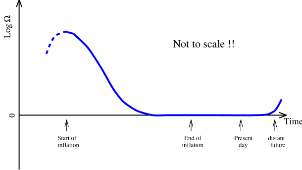
Figure 1: A possible evolution of $\Omega$. There may or may not be evolution before inflation, shown by the dotted line. During inflation $\Omega$ is forced dramatically towards one, and remains there right up to the present. Only in the extremely distant future will it begin to evolve away from one again.

In the above discussion, I have ignored a possible cosmological constant contribution, but if present it modifies the Friedmann equation to

$$\left|\Omega+\Omega_{\Lambda}-1\right|=\frac{|k|}{a^{2}H^{2}}\,,$$ (31)

and so it is $\Omega+\Omega_{\Lambda}$ which is forced to one. In general, it is spatial flatness ($k\simeq 0$) that we are driven towards, not a critical matter density.

4.2 Relic abundances

The rapid expansion of the inflationary stage rapidly dilutes the unwanted relic particles, because the energy density during inflation falls off more slowly (as $a^{-2}$ or slower) than the relic particle density. Very quickly their density becomes negligible.

This resolution can only work if, after inflation, the energy density of the Universe can be turned into conventional matter without recreating the unwanted relics. This can be achieved by ensuring that during the conversion, known as reheating, the temperature never gets hot enough again to allow their thermal recreation. Then reheating can generate solely the things which we want. Such successful reheating allows us to get back into the hot big bang Universe, recovering all its later successes such as nucleosynthesis and the microwave background.

4.3 The horizon problem and homogeneity

The inflationary expansion also solves the horizon problem. The basic strategy is to ensure that

$$\int_{t_{*}}^{t_{{\rm dec}}}\frac{dt}{a(t)}\gg\int_{t_{{\rm dec}}}^{t_{0}}\frac{dt}{a(t)}\,,$$ (32)

so that light can travel much further before decoupling than it can afterwards. This cannot be done with standard evolution, but can be achieved by inflation.

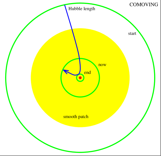
Figure 2: Solving the horizon problem. Initially the Hubble length is large, and a smooth patch forms by causal interactions. Inflation then shrinks the Hubble length, and even the subsequent expansion again after inflation leaves the observable Universe within the smoothed patch.

An alternative way to view this is to remember that inflation corresponds to a decreasing comoving Hubble length. The Hubble length is ordinarily a good measure of how far things can travel in the Universe; what this is telling us is that the region of the Universe we can see after (even long after) inflation is much smaller than the region which would have been visible before inflation started. Hence causal physics was perfectly capable of producing a large smooth thermalized region, encompassing a volume greatly in excess of our presently observable Universe. In Figure 2, the outer circle indicates the initial Hubble length, encompassing the shaded smooth patch. Inflation shrinks this dramatically inwards towards the dot indicating our position, and then after inflation it increases while staying within the initial smooth patch.

Equally, causal processes would be capable of generating irregularities in the Universe on scales greatly exceeding our presently observable Universe, provided they happened at an early enough time that those scales were within causal contact. This will be explored in detail later.

5 Modelling the Inflationary Expansion

We have seen that a period of accelerated expansion — inflation — is sufficient to resolve a range of cosmological problems. But we need a plausible scenario for driving such an expansion if we are to be able to make proper calculations. This is provided by cosmological scalar fields.

5.1 Scalar fields and their potentials

In particle physics, a scalar field is used to represent spin zero particles. It transforms as a scalar (that is, it is unchanged) under coordinate transformations. In a homogeneous Universe, the scalar field is a function of time alone.

In particle theories, scalar fields are a crucial ingredient for spontaneous symmetry breaking. The most famous example is the Higgs field which breaks the electro-weak symmetry, whose existence is hoped to be verified at the Large Hadron Collider at CERN when it commences experiments next millennium. Scalar fields are also expected to be associated with the breaking of other symmetries, such as those of Grand Unified Theories, supersymmetry etc.

• Any specific particle theory (eg GUTS, superstrings) contains scalar fields.

• No fundamental scalar field has yet been observed.

• In condensed matter systems (such as superconductors, superfluid helium etc) scalar fields are widely observed, associated with any phase transition. People working in that subject normally refer to the scalar fields as ‘order parameters’.

The traditional starting point for particle physics models is the action, which is an integral of the Lagrange density over space and time and from which the equations of motion can be obtained. As an intermediate step, one might write down the energy–momentum tensor, which sits on the right-hand side of Einstein’s equations. Rather than begin there, I will take as my starting point expressions for the effective energy density and pressure of a homogeneous scalar field, which I’ll call $\phi$. These are obtained by comparison of the energy–momentum tensor of the scalar field with that of a perfect fluid, and are

$$\rho_{\phi} = \frac{1}{2}\dot{\phi}^{2}+V(\phi)\,$$ (33)

$$p_{\phi} = \frac{1}{2}\dot{\phi}^{2}-V(\phi)\,.$$ (34)

One can think of the first term in each as a kinetic energy, and the second as a potential energy. The potential energy $V(\phi)$ can be thought of as a form of ‘configurational’ or ‘binding’ energy; it measures how much internal energy is associated with a particular field value. Normally, like all systems, scalar fields try to minimize this energy; however, a crucial ingredient which allows inflation is that scalar fields are not always very efficient at reaching this minimum energy state.

Note in passing that a scalar field cannot in general be described by an equation of state; there is no unique value of $p$ that can be associated with a given $\rho$ as the energy density can be divided between potential and kinetic energy in different ways.

In a given theory, there would be a specific form for the potential $V(\phi)$, at least up to some parameters which one could hope to measure (such as the effective mass and interaction strength of the scalar field). However, we are not presently in a position where there is a well established fundamental theory that one can use, so, in the absence of such a theory, inflation workers tend to regard $V(\phi)$ as a function to be chosen arbitrarily, with different choices corresponding to different models of inflation (of which there are many). Some example potentials are

$$V(\phi)=\lambda\left(\phi^{2}-M^{2}\right)^{2}\quad\quad$$ Higgs potential (35)

$$V(\phi)=\frac{1}{2}m^{2}\phi^{2}$$ Massive scalar field (36)

$$V(\phi)=\lambda\phi^{4}$$ Self-interacting scalar field (37)

The strength of this approach is that it seems possible to capture many of the crucial properties of inflation by looking at some simple potentials; one is looking for results which will still hold when more ‘realistic’ potentials are chosen. Figure 3 shows such a generic potential, with the scalar field displaced from the minimum and trying to reach it.

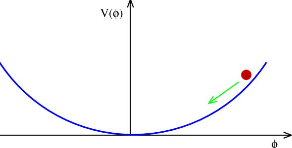
Figure 3: A generic inflationary potential.

5.2 Equations of motion and solutions

The equations for an expanding Universe containing a homogeneous scalar field are easily obtained by substituting Eqs. (33) and (34) into the Friedmann and fluid equations, giving

$$H^{2} = \frac{8\pi}{3m_{{\rm Pl}}^{2}}\left[V(\phi)+\frac{1}{2}\dot{\phi}^{2}\right]\,,$$ (38)

$$\ddot{\phi}+3H\dot{\phi} = -V^{\prime}(\phi)\,,$$ (39)

where prime indicates $d/d\phi$. Here I have ignored the curvature term $k$, since we know that by definition it will quickly become negligible once inflation starts. This is done for simplicity only; there is no obstacle to including that term.

Since

$$\ddot{a}>0\Longleftrightarrow p<-\frac{\rho}{3}\Longleftrightarrow\dot{\phi}^{2}<V(\phi)$$ (40)

we will have inflation whenever the potential energy dominates. This should be possible provided the potential is flat enough, as the scalar field would then be expected to roll slowly. The potential should also have a minimum in which inflation can end.

The standard strategy for solving these equations is the slow-roll approximation (SRA); this assumes that a term can be neglected in each of the equations of motion to leave the simpler set

$$H^{2} \simeq \frac{8\pi}{3m_{{\rm Pl}}^{2}}\,V$$ (41)

$$3H\dot{\phi} \simeq -V^{\prime}$$ (42)

If we define slow-roll parameters [3]

$$\epsilon(\phi)=\frac{m_{{\rm Pl}}^{2}}{16\pi}\,\left(\frac{V^{\prime}}{V}\right)^{2}\quad;\quad\eta(\phi)=\frac{m_{{\rm Pl}}^{2}}{8\pi}\,\frac{V^{\prime\prime}}{V}\,,$$ (43)

where the first measures the slope of the potential and the second the curvature, then necessary conditions for the slow-roll approximation to hold are 

$$\epsilon\ll 1\quad;\quad|\eta|\ll 1\,.$$ (44)

Unfortunately, although these are necessary conditions for the slow-roll approximation to hold, they are not sufficient, since even if the potential is very flat it may be that the scalar field has a large velocity. A more elaborate version of the SRA exists, based on the Hamilton–Jacobi formulation of inflation,[4] which is sufficient as well as necessary.[5]

Note also that the SRA reduces the order of the system of equations by one, and so its general solution contains one less initial condition. It works only because one can prove [4, 5] that the solution to the full equations possesses an attractor property, eliminating the dependence on the extra parameter.

5.3 The relation between inflation and slow-roll

As it happens, the applicability of the slow-roll condition is closely connected to the condition for inflation to take place, and in many contexts the conditions can be regarded as equivalent. Let’s quickly see why.

The inflationary condition $\ddot{a}>0$ is satisfied for a much wider range of behaviours than just (quasi-)exponential expansion. A classic example is power-law inflation $a\propto t^{p}$ for $p>1$, which is an exact solution for an exponential potential

$$V(\phi)=V_{0}\exp\left[-\sqrt{\frac{16\pi}{p}}\,\frac{\phi}{m_{{\rm Pl}}}\right]\,.$$ (45)

We can manipulate the condition for inflation as

$$\frac{\ddot{a}}{a}=\dot{H}+H^{2}>0$$

$$\Longleftrightarrow -\frac{\dot{H}}{H^{2}}<1$$

$$\stackrel{{\scriptstyle\sim}}{{\Longleftrightarrow}} \frac{m_{{\rm Pl}}^{2}}{16\pi}\,\left(\frac{V^{\prime}}{V}\right)^{2}<1$$

where the last manipulation uses the slow-roll approximation. The final condition is just the slow-roll condition $\epsilon<1$, and hence

$$\mbox{Slow-roll}\Longrightarrow\mbox{Inflation}$$

Inflation will occur when the slow-roll conditions are satisfied (subject to some caveats on whether the ‘attractor’ behaviour has been attained.[5])

However, the converse is not strictly true, since we had to use the SRA in the derivation. However, in practice

Inflation $$\stackrel{{\scriptstyle\sim}}{{\Longrightarrow}} \epsilon<1$$

Prolonged inflation $$\stackrel{{\scriptstyle\sim}}{{\Longrightarrow}} \eta<1$$

The last condition arises because unless the curvature of the potential is small, the potential will not be flat for a wide enough range of $\phi$.

5.4 The amount of inflation

The amount of inflation is normally specified by the logarithm of the amount of expansion, the number of e-foldings $N$, given by

$$N\equiv\ln\frac{a(t_{{\rm end}})}{a(t_{{\rm initial}})} = \int_{t_{{\rm i}}}^{t_{{\rm e}}}\,H\,dt\,,$$ (46)

$$\simeq -\frac{8\pi}{m_{{\rm Pl}}^{2}}\int_{\phi_{{\rm i}}}^{\phi_{{\rm e}}}\,\frac{V}{V^{\prime}}\,d\phi\,,$$ (47)

where the final step uses the SRA. Notice that the amount of inflation between two scalar field values can be calculated without needing to solve the equations of motion, and also that it is unchanged if one multiplies $V(\phi)$ by a constant.

The minimum amount of inflation required to solve the various cosmological problems is about 70 $e$-foldings, i.e. an expansion by a factor of $10^{30}$. Although this looks large, inflation is typically so rapid that most inflation models give much more.

5.5 A worked example: polynomial chaotic inflation

The simplest inflation model [6] arises when one chooses a polynomial potential, such as that for a massive but otherwise non-interacting field, $V(\phi)=m^{2}\phi^{2}/2$ where $m$ is the mass of the scalar field. With this potential, the slow-roll equations are

$$3H\dot{\phi}+m^{2}\phi=0\quad;\quad H^{2}=\frac{4\pi m^{2}\phi^{2}}{3m_{{\rm Pl}}^{2}}\,,$$ (48)

and the slow-roll parameters are

$$\epsilon=\eta=\frac{m_{{\rm Pl}}^{2}}{4\pi\phi^{2}}\,.$$ (49)

So inflation can proceed provided $|\phi|>m_{{\rm Pl}}/\sqrt{4\pi}$, i.e. as long as we are not to close to the minimum.

The slow-roll equations are readily solved to give

$$\phi(t) = \phi_{{\rm i}}-\frac{m\,m_{{\rm Pl}}}{\sqrt{12\pi}}\,t\,,$$ (50)

$$a(t) = a_{{\rm i}}\exp\left[\sqrt{\frac{4\pi}{3}}\,\frac{m}{m_{{\rm Pl}}}\,\left(\phi_{{\rm i}}t-\frac{m\,m_{{\rm Pl}}}{\sqrt{48\pi}}t^{2}\right)\right]\,,$$ (51)

(where $\phi=\phi_{{\rm i}}$ and $a=a_{{\rm i}}$ at $t=0$) and the total amount of inflation is

$$N_{{\rm tot}}=2\pi\,\frac{\phi_{{\rm i}}^{2}}{m_{{\rm Pl}}^{2}}-\frac{1}{2}\,.$$ (52)

This last equation can be obtained from the solution for $a$, but in fact is more easily obtained directly by integrating Eq. (47), for which one needn’t bother to solve the equations of motion.

In order for classical physics to be valid we require $V\ll m_{{\rm Pl}}^{4}$, but it is still easy to get enough inflation provided $m$ is small enough. As we shall later see, $m$ is in fact required to be small from observational limits on the size of density perturbations produced, and we can easily get far more than the minimum amount of inflation required to solve the various cosmological problems we originally set out to solve.

5.6 Reheating after inflation

During inflation, all matter except the scalar field (usually called the inflaton) is redshifted to extremely low densities. Reheating is the process whereby the inflaton’s energy density is converted back into conventional matter after inflation, re-entering the standard big bang theory.

Once the slow-roll conditions break down, the scalar field switches from being overdamped to being underdamped and begins to move rapidly on the Hubble timescale, oscillating at the bottom of the potential. As it does so, it decays into conventional matter. The details of reheating are an important area of research in inflationary cosmology at the moment for several reasons, but are not important for the generation and evolution of density perturbations which is the main focus of the remainder of this article. Consequently, I’ll just note that recently there has been quite a dramatic change of view as to how reheating takes place. Traditional treatments (e.g. as given in Kolb & Turner [7]) added a phenomenological decay term; this was constrained to be very small and hence reheating was viewed as being very inefficient. This allowed substantial redshifting to take place after the end of inflation and before the Universe returned to thermal equilibrium; hence the reheat temperature would be lower, by several orders of magnitude, than suggested by the energy density at the end of inflation.

This picture is radically revised in work by Kofman, Linde & Starobinsky [8] (see also Ref. [9]), who suggest that the decay can undergo broad parametric resonance, with extremely efficient transfer of energy from the coherent oscillations of the inflaton field. This initial transfer has been dubbed preheating. With such an efficient start to the reheating process, it now appears possible that the reheating epoch may be very short indeed and hence that most of the energy density in the inflaton field at the end of inflation may be available for conversion into thermalized form.

5.7 The range of inflation models

Over the last fifteen years or so a great number of inflationary models have been devised, both with and without reference to specific underlying particle theories. Here I will discuss a very small subset of the models which have been introduced, just to give you a flavour of the variety. At the moment particle physics model building of inflation is undergoing a renaissance, and a detailed snapshot of the current situation can be found in the review of Lyth & Riotto.[10]

However, as we shall be discussing in the next section, observations have great prospects for distinguishing between the different inflationary models. By far the best type of observation for this purpose appears to be high resolution satellite microwave background anisotropy observations, and we are fortunate that two proposals have been approved — NASA has funded the MAP satellite [11] for launch around 2000, and ESA has approved the Planck satellite [12] for launch some later. These satellites should offer very strong discrimination between the inflation models I shall now discuss. Indeed, it may even be possible to attempt a more challenging type of observation — one which is independent of the particular inflationary model and hence begins to test the idea of inflation itself.

5.7.1 Chaotic inflation models

This is the standard type of inflation model.[6] The ingredients are

• A single scalar field, rolling in …

• A potential $V(\phi)$, which in some regions satisfies the slow-roll conditions, while also possessing a minimum with zero potential in which inflation is to end.

• Initial conditions well up the potential, due to large fluctuations at the Planck era.

There are a large number of models of this type. Some are

Polynomial chaotic inflation	$V(\phi)=\frac{1}{2}m^{2}\phi^{2}$
	$V(\phi)=\lambda\phi^{4}$
Power-law inflation	$V(\phi)=V_{0}\exp(\sqrt{\frac{16\pi}{p}}\,\frac{\phi}{m_{{\rm Pl}}})$
‘Natural’ inflation	$V(\phi)=V_{0}[1+\cos\frac{\phi}{f}]$
Intermediate inflation	$V(\phi)\propto\phi^{-\beta}$

Some of these actually do not satisfy the condition of a minimum in which inflation ends; they permit inflation to continue forever. However, we shall see power-law inflation arising in a more satisfactory context shortly.

5.7.2 Multi-field theories

A recent trend in inflationary model building has been the exploration of models with more than one scalar field. The classic example is the hybrid inflation model,[13] which seems particularly promising for particle physics model building. The simplest version has a potential with two fields $\phi$ and $\psi$ of the form

$$V(\phi,\psi)=\frac{\lambda}{4}\left(\psi^{2}-M^{2}\right)^{2}+\frac{1}{2}m^{2}\phi^{2}+\frac{1}{2}\lambda^{\prime}\phi^{2}\psi^{2}\,.$$ (53)

which is illustrated in Figure 4. When $\phi^{2}$ is large, the minimum of the potential in the $\psi$-direction is at $\psi=0$. The field rolls down this ‘channel’ until it reaches $\phi_{{\rm inst}}^{2}=\lambda M^{2}/\lambda^{\prime}$, at which point $\psi=0$ becomes unstable and the field rolls into one of the true minima at $\phi=0$ and $\psi=\pm M$.

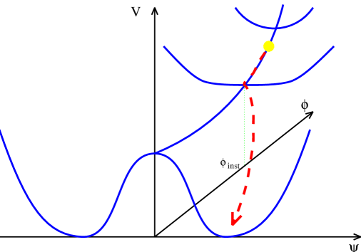
Figure 4: The potential for the hybrid inflation model. The field rolls down the channel at $\psi=0$ until it reaches the critical $\phi$ value, then falls off the side to the true minimum at $\phi=0$ and $\psi=\pm M$.

While in the ‘channel’, which is where all the interesting behaviour takes place, this is just like a single field model with an effective potential for $\phi$ of the form

$$V_{{\rm eff}}(\phi)=\frac{\lambda}{4}M^{4}+\frac{1}{2}m^{2}\phi^{2}\,.$$ (54)

This is a fairly standard form, the unusual thing being the constant term, which would not normally be allowed as it would give a present-day cosmological constant. The most interesting regime is where that constant dominates, and it gives quite an unusual phenomenology. In particular, the energy density during inflation can be much lower than normal while still giving suitably large density perturbations, and secondly the field $\phi$ can be rolling extremely slowly which is of benefit to particle physics model building.

Within the more general class of two and multi-field inflation models, it is quite common for only one field to be dynamically important, as in the hybrid inflation model — this effectively reduces the situation back to the single field case of the previous subsection. However, it may also be possible to have more than one important dynamical degree of freedom. In that case there is no attractor behaviour giving a unique route into the potential minimum, as in the single field case; for example, if the potential is of the form of an asymmetric bowl one could roll into the base down any direction. In that situation, the model loses some of its predictive power, because the late-time behaviour is not independent of the initial conditions.

5.7.3 Beyond general relativity

Rather than introduce an explicit scalar field to drive inflation, some theories modify the gravitational sector of the theory into something more complicated than general relativity.[14] Examples are

• Higher derivative gravity ($R+R^{2}+\cdots$).

• Jordan–Brans–Dicke theory.

• Scalar–tensor gravity.

The last two are theories where the gravitational constant may vary (indeed Jordan–Brans–Dicke theory is a special case of scalar–tensor gravity).

However, a clever trick, known as the conformal transformation,[15] allows such theories to be rewritten as general relativity plus one or more scalar fields with some potential. Often, only one of those fields is dynamical which returns us once more to the original chaotic inflation scenario!

The most famous example is extended inflation.[16] In its original form, it transforms precisely into the power-law inflation model that we’ve already discussed, with the added bonus that it includes a proper method of ending inflation. Unfortunately though, this model is now ruled out by observations.[3] Indeed, models of inflation based on altering gravity are much more constrained than other types, since we know a lot about gravity and how well general relativity works,[14] and many models of this kind are very vulnerable to observations.

5.7.4 Open inflation

In the early 1990s, in the face of ever increasing evidence of a sub-critical matter density in the Universe, interest was refocussed on an idea which defies the original inflationary motivation and gives rise to a homogeneous but open Universe from inflation. Often in the past it has been declared that this is either impossible or contrived; however, it can be readily achieved in models with quantum tunnelling from a false vacuum (a metastable state) followed by a second inflationary stage.[17] The tunnelling creates a bubble, and, incredibly, the region inside the expanding bubble looks just like an open Universe, with the bubble wall corresponding to the initial (coordinate) singularity. These models are normally referred to as ‘open inflation’ or ‘single-bubble’ models. So far it has turned out that such models are not all that easy to construct.

These models are already very different from traditional inflation models, and subsequently an even bolder idea has been proposed,[18] that an open Universe can be created via ‘tunnelling from nothing’ rather than from a pre-existing inflationary phase. As I write this remains controversial.

While both these types of open inflation models remain viable, they are considerably more complex than the standard inflation models, and at the moment not that well motivated as although observations continue to favour a low matter density, they also favour spatial flatness reintroduced by a cosmological constant. Therefore from now on I will restrict discussion to the single-field chaotic inflation models.

5.8 Recap

The main points of this long section were the following.

• Cosmological scalar fields, which were introduced long before inflation was thought of, provide a natural framework for inflation.

• Despite a wide range of motivations, most inflationary models are dynamically equivalent to general relativity plus a single scalar field with some potential $V(\phi)$.

• Within this framework, solutions describing inflation are easily found. Indeed, for many of the properties (amount of expansion, for example), we do not even need to solve the equations of motion.

With this information under our belts, we are now able to discuss the strongest motivation for the inflationary cosmology — that it is able to provide an explanation for the origin of structure in the Universe.

6 Density Perturbations and Gravitational Waves

In modern terms, by far the most important property of inflationary cosmology is that it produces spectra of both density perturbations and gravitational waves. The density perturbations may be responsible for the formation and clustering of galaxies, as well as creating anisotropies in the microwave background radiation. The gravitational waves do not affect the formation of galaxies, but as we shall see may contribute extra microwave anisotropies on the large angular scales sampled by the COBE satellite.[19, 20] An alternative terminology for the density perturbations is scalar perturbations and for the gravitational waves is tensor perturbations, the terminology referring to their transformation properties.

Studies of large-scale structure typically make some assumption about the initial form of these spectra. Usually gravitational waves are assumed not to be present, and the density perturbations to take on a simple form such as the scale-invariant Harrison–Zel’dovich spectrum, or a scale-free power-law spectrum. It is clearly highly desirable to have a theory which predicts the forms of the spectra. There are presently two rival models which do this, cosmological inflation and topological defects. At present inflation is favoured both on observational grounds and because it provides a simpler framework for understanding the evolution of structure

6.1 Production during inflation

The ability of inflation to generate perturbations on large scales comes from the unusual behaviour of the Hubble length during inflation, namely that (by definition) the comoving Hubble length decreases. When we talk about large-scale structure, we are primarily interested in comoving scales, as to a first approximation everything is dragged along with the expansion. The qualitative behaviour of irregularities is governed by their scale in comparison to the characteristic scale of the Universe, the Hubble length.

In the big bang Universe the comoving Hubble length is always increasing, and so all scales are initially much larger than it, and hence unable to be affected by causal physics. Once they become smaller than the Hubble length, they remain so for all time. In the standard scenarios, COBE sees perturbations on large scales at a time when they were much bigger than the Hubble length, and hence no mechanism could have created them.

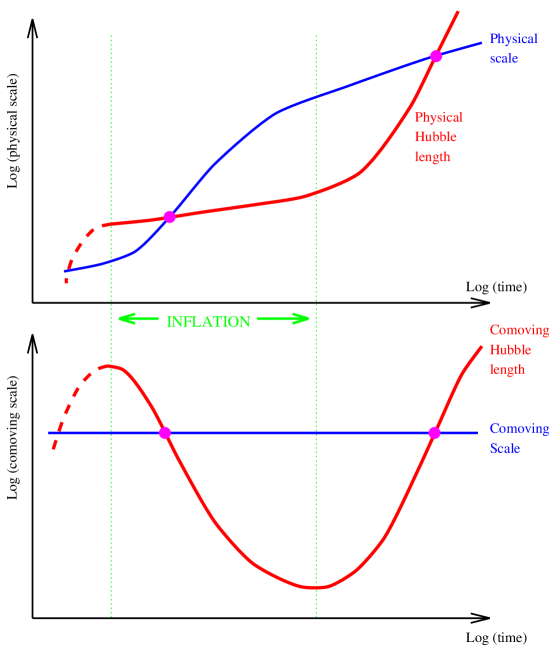
Figure 5: The behaviour of a given comoving scale relative to the Hubble length, both during and after inflation, shown using physical coordinates (upper panel) and comoving ones (lower panel).

Inflation reverses this behaviour, as seen in Figure 5. Now a given comoving scale has a more complicated history. Early on in inflation, the scale could be well inside the Hubble length, and hence causal physics can act, both to generate homogeneity to solve the horizon problem and to superimpose small perturbations. Some time before inflation ends, the scale crosses outside the Hubble radius (indicated by a circle in the lower panel of Figure 5) and causal physics becomes ineffective. Any perturbations generated become imprinted, or, in the usual terminology, ‘frozen in’. Long after inflation is over, the scales cross inside the Hubble radius again. Perturbations are created on a very wide range of scales, but the most readily observed ones range from about the size of the present Hubble radius (i.e. the size of the presently observable Universe) down to a few orders of magnitude less. On the scale of Figure 5, all interesting comoving scales lie extremely close together, and cross the Hubble radius during inflation very close together.

It’s all very well to realize that the dynamics of inflation permits perturbations to be generated without violating causality, but we need a specific mechanism. That mechanism is quantum fluctuations. Inflation is trying as hard as it can to make the Universe perfectly homogeneous, but it cannot defeat the Uncertainty Principle which ensures that there are always some irregularities left over. Through this limitation, it is possible for inflation to adequately solve the homogeneity problem and in addition leave enough irregularities behind to attempt to explain why the present Universe is not completely homogeneous.

The size of the irregularities depends on the energy scale at which inflation takes place. It is outside the scope of these lectures to describe in detail how this calculation is performed (see e.g. Ref. [21] for a reasonably accessible description); I’ll just briefly outline the necessary steps and then quote the result, which we can go on to apply.

(a) Perturb the scalar field	$\phi=\phi(t)+\delta\!\phi({\bf x},t)$
(b) Expand in comoving wavenumbers	$\delta\phi=\sum(\delta\!\phi)_{{\bf k}}e^{i{\bf k}.{\bf x}}$
(c) Linearized equation for classical evolution
(d) Quantize theory
(e) Find solution with initial condition giving
flat space quantum theory ($k\gg aH$)
(f) Find asymptotic value for $k\ll aH$	$\langle|\delta\!\phi_{{\bf k}}|^{2}\rangle=H^{2}/2k^{3}$
(g) Relate field perturbation to metric	${\cal R}=H\,\delta\!\phi/\dot{\phi}$
or curvature perturbation

Some important points are

• The details of this calculation are extremely similar to those used to calculate the Casimir effect (a quantum force between parallel plates), which has been tested in the laboratory.

• The calculation itself is not controversial, though some aspects of its interpretation (in particular concerning the quantum to classical transition) are.

• Exact analytic results are not known for general inflation models (though linear theory results for arbitrary models are readily calculated numerically [22]). The results I’ll be quoting will be lowest-order in the SRA, which is good enough for present observations.

• Results are known to second-order in slow-roll for arbitrary inflaton potentials.[23] Power-law inflation is the only standard model for which exact results are known. In some other cases, high accuracy approximations give better results (e.g. small-angle approximation in natural or hybrid inflation [23, 24]).

The formulae for the amplitude of density perturbations, which I’ll call $\delta_{{\rm H}}(k)$, and the gravitational waves, $A_{{\rm G}}(k)$, are 

$$\delta_{{\rm H}}(k) = \left.\sqrt{\frac{512\pi}{75}}\,\frac{V^{3/2}}{m_{{\rm Pl}}^{3}|V^{\prime}|}\right|_{k=aH}\,,$$ (55)

$$A_{{\rm G}}(k) = \left.\sqrt{\frac{32}{75}}\,\frac{V^{1/2}}{m_{{\rm Pl}}^{2}}\right|_{k=aH}\,.$$ (56)

Here $k$ is the comoving wavenumber; the perturbations are normally analyzed via a Fourier expansion into comoving modes. The right-hand sides of the above equations are to be evaluated at the time when $k=aH$ during inflation, which for a given $k$ corresponds to some particular value of $\phi$. We see that the amplitude of perturbations depends on the properties of the inflaton potential at the time the scale crossed the Hubble radius during inflation. The relevant number of $e$-foldings from the end of inflation is given by [2]

$$N\simeq 62-\ln\frac{k}{a_{0}H_{0}}+\mbox{numerical correction}\,,$$ (57)

where ‘numerical correction’ is a typically smallish (order a few) number which depends on the energy scale of inflation, the duration of reheating and so on. Normally it is a perfectly fine approximation to say that the scales of interest to us crossed outside the Hubble radius 60 $e$-foldings before the end of inflation. Then the $e$-foldings formula

$$N\simeq-\frac{8\pi}{m_{{\rm Pl}}^{2}}\int_{\phi}^{\phi_{{\rm end}}}\,\frac{V}{V^{\prime}}\,d\phi\,,$$ (58)

tells us the value of $\phi$ to be substituted into Eqs. (55) and (56).

6.2 A worked example

The easiest way to see what is going on is to work through a specific example, the $m^{2}\phi^{2}/2$ potential which we already saw in Section 5.5. We’ll see that we don’t even have to solve the evolution equations to get our predictions.

1. Inflation ends when $\epsilon=1$, so $\phi_{{\rm end}}\simeq m_{{\rm Pl}}/\sqrt{4\pi}$.

2. We’re interested in 60 $e$-foldings before this, which from Eq. (52) gives $\phi_{60}\simeq 3m_{{\rm Pl}}$.

3. Substitute this in:

   $$\delta_{{\rm H}}\simeq 12\,\frac{m}{m_{{\rm Pl}}}\quad;\quad A_{{\rm G}}\simeq 1.4\,\frac{m}{m_{{\rm Pl}}}$$

4. Reproducing the COBE result requires [25] $\delta_{{\rm H}}\simeq 2\times 10^{-5}$ (provided $A_{{\rm G}}\ll\delta_{{\rm H}}$), so we need $m\simeq 10^{-6}m_{{\rm Pl}}$.

Because the required value of $m$ is so small, that means it is easy to get sufficient inflation to solve the cosmological problems, without violating the classicality condition $V<m_{{\rm Pl}}^{4}$. That implies only that $\phi<m_{{\rm Pl}}^{2}/m\simeq 10^{6}m_{{\rm Pl}}$, and as $N_{{\rm tot}}\simeq 2\pi\phi^{2}/m_{{\rm Pl}}^{2}$, we can get up to about $10^{13}$ $e$-foldings in principle. This compares extremely favourably with the 70 or so actually required.

6.3 Observational consequences

Observations have moved on beyond us wanting to know the overall normalization of the potential. The interesting things are

1. The scale-dependence of the spectra.

2. The relative influence of the two spectra.

These can be neatly summarized using the slow-roll parameters $\epsilon$ and $\eta$ we defined earlier.[3]

The standard approximation used to describe the spectra is the power-law approximation, where we take

$$\delta_{{\rm H}}^{2}(k)\propto k^{n-1}\quad;\quad A_{{\rm G}}^{2}(k)\propto k^{n_{{\rm G}}}\,,$$ (59)

where the spectral indices $n$ and $n_{{\rm G}}$ are given by

$$n-1=\frac{d\ln\delta_{{\rm H}}^{2}}{d\ln k}\quad;\quad n_{{\rm G}}=\frac{d\ln A_{{\rm G}}^{2}}{d\ln k}\,.$$ (60)

The power-law approximation is usually valid because only a limited range of scales are observable, with the range $1$ Mpc to $10^{4}$ Mpc corresponding to $\Delta\ln k\simeq 9$.

The crucial equation we need is that relating $\phi$ values to when a scale $k$ crosses the Hubble radius, which from Eq. (58) is

$$\frac{d\ln k}{d\phi}=\frac{8\pi}{m_{{\rm Pl}}^{2}}\,\frac{V}{V^{\prime}}\,.$$ (61)

(since within the slow-roll approximation $k\simeq\exp N$). Direct differentiation then yields [3]

$$n = 1-6\epsilon+2\eta\,,$$ (62)

$$n_{{\rm G}} = -2\epsilon\,,$$ (63)

where now $\epsilon$ and $\eta$ are to be evaluated on the appropriate part of the potential.

Finally, we need a measure of the relevant importance of density perturbations and gravitational waves. The natural place to look is the microwave background; a detailed calculation which I cannot reproduce here (see e.g. Ref. [2]) gives

$$R\equiv\frac{C_{\ell}^{{\rm GW}}}{C_{\ell}^{{\rm DP}}}\simeq\,4\pi\epsilon\,.$$ (64)

Here the $C_{\ell}$ are the contributions to the microwave multipoles, in the usual notation.

From these expressions we immediately see

• If and only if $\epsilon\ll 1$ and $|\eta|\ll 1$ do we get $n\simeq 1$ and $R\simeq 0$.

• Because the coefficient in Eq. (64) is so large, gravitational waves can have a significant effect even if $\epsilon$ is quite a bit smaller than one.

Table 1 shows the predictions for a range of inflation models. The information I’ve given you so far should be sufficient to allow you to reproduce them. Even the simplest inflation models can affect the large-scale structure modelling at a level comparable to the present observational accuracy. The predictions of the different models will be wildly different as far as future high-accuracy observations are concerned.

MODEL	POTENTIAL	$n$	$R$
Polynomial	$\phi^{2}$	0.97	0.1
chaotic inflation	$\phi^{4}$	0.95	0.2
Power-law inflation	$\exp(-\lambda\phi)$	any $n<1$	$2\pi(1-n)$
‘Natural’ inflation	$1+\cos(\phi/f)$	any $n<1$	0
Hybrid inflation (standard)	$1+B\phi^{2}$	1	0
Hybrid inflation (extreme)	$1+B\phi^{2}$	$1<n<1.15$	$\sim 0$

Table 1: The spectral index and gravitational wave contribution for a range of inflation models.

Observations have some way to go before the power-law approximation becomes inadequate. Consequently …

• Slow-roll inflation adds two, and only two, new parameters to large-scale structure.

• Although $\epsilon$ and $\eta$ are the fundamental parameters, it is best to take them as $n$ and $R$.

• Inflation models predict a wide range of values for these. Hence inflation makes no definite prediction for large-scale structure.

• However, this means that large-scale structure observations, and especially microwave background observations, can strongly discriminate between inflationary models. When they are made, most existing inflation models will be ruled out.

6.4 Testing the idea of inflation

The moral of the previous section was that different inflation models lead to very different models of structure formation, spanning a wide range of possibilities. That means, for example, that a definite measure of say the spectral index $n$ would rule out most inflation models. But it would always be possible to find models which did give that value of $n$. Is there any way to try and test the idea of inflation, independently of the model chosen?

The answer, in principle, is yes. In the previous section we introduced three observables (in addition to the overall normalization), namely $n$, $R$ and $n_{{\rm G}}$. However, they depend only on two fundamental parameters, namely $\epsilon$ and $\eta$.[3] We can therefore eliminate $\epsilon$ and $\eta$ to obtain a relation between observables, the consistency equation

$$R=-2\pi n_{{\rm G}}\,.$$ (65)

This relation has been much discussed in the literature.[26, 21] It is independent of the choice of inflationary model (though it does rely on the slow-roll and power-law approximations).

The idea of a consistency equation is in fact very general. The point is that we have obtained two continuous functions, $\delta_{{\rm H}}(k)$ and $A_{{\rm G}}(k)$, from a single continuous function $V(\phi)$. This can only be possible if the functions $\delta_{{\rm H}}(k)$ and $A_{{\rm G}}(k)$ are related, and the equation quoted above is the simplest manifestation of such a relation.

Vindication of the consistency equation would be a remarkably convincing test of the inflationary paradigm, as it would be highly unlikely that any other production mechanism could entangle the two spectra in the way inflation does. Unfortunately though, measuring $n_{{\rm G}}$ is a much more challenging observational task than measuring $n$ or $R$ and is likely to be beyond even next generation observations. Indeed, this is a good point to remind the reader that even if inflation is right, only one model can be right and it is perfectly possible (and maybe even probable, see Ref. [27]) that that model has a very low amplitude of gravitational waves and that they will never be detected.

7 The inflationary origin of structure

At the summer school where these lectures were given, models of structure formation were described in detail by Joe Silk and for a detailed treatment I refer you to his corresponding article. Here I will address those issues of direct relevance to the inflationary cosmology.

7.1 The parameters

The initial goal of structure formation studies is to accurately determine the fundamental parameters describing our Universe. So far I’ve stressed the three inflationary parameters, $\delta_{{\rm H}}$, $n$ and $r$, which describe the initial perturbations which inflation generates. However, except on very large scales where they remain untouched by causal processes, we do not see the original perturbations but rather than perturbations after they have been processed by a variety of physical mechanisms. This processing depends on many quantities, all of which must be either fixed by assumption or determined from observations. A basic list features four categories; the global dynamics, the way in which the matter content is divided amongst the different particle species, astrophysics effects such as reionization which would affect the microwave background photons, and the initial perturbation spectrum that we are here assuming comes from inflation. A possible list might look like this

1. Global dynamics

   Hubble constant $h$           $*$

   Spatial curvature $k$

2. Matter content

   Baryons $\Omega_{{\rm B}}$           $*$

   Hot dark matter? $\Omega_{{\rm HDM}}$

   Cosmological constant? $\Lambda$           $(*)$

   Massless species? $g_{*}$

3. Astrophysics

   Reionization optical depth $\tau$           $*$

4. Initial perturbations

   Amplitude $\delta_{{\rm H}}(k=a_{0}H_{0})$           $*$

   Spectral index $n$           $*$

   Gravitational waves $r$

A cold dark matter contribution is not mentioned under matter content as it is assumed to take the value required to make the sums add up (i.e. to give the right spatial curvature $k$ given the other matter densities).

In this list, I’ve starred those parameters which need to be included in even the most minimal model, while the rest can be set to some particular value by assumption. I’ve partially starred the cosmological constant because although most people would like to set it to zero, the observational case for a non-zero value is near to overwhelming.

7.2 The inflationary energy scale

The most solid observational result is the interpretation of the cosmic microwave anisotropies seen by COBE as giving the amplitude of the initial power spectrum. COBE is a particularly powerful probe because its large beam size makes it sensitive only to scales much larger than the horizon size when the microwave background formed. The perturbations are therefore seen in their primordial form, and depend only on the initial perturbations and not all the other parameters. 

The COBE normalization requires the perturbation at the present Hubble scale, $\delta_{{\rm H}}\equiv\delta_{{\rm H}}(k=a_{0}H_{0})$, to be given by [25]

$$\delta_{{\rm H}}\simeq 2\times 10^{-5}\,.$$ (66)

Since

$$\delta_{{\rm H}}^{2}=\frac{32}{75}\,\frac{V}{m_{{\rm Pl}}^{4}}\,\frac{1}{\epsilon}\,,$$ (67)

then unless $\epsilon$ proves to be tiny (say much less than a hundredth) this will give

$$V^{1/4}\simeq 10^{-3}m_{{\rm Pl}}\simeq 10^{16}\,{\rm GeV}\,,$$ (68)

at the time when observable scales crossed outside the horizon, pretty much the scale that particle physicists associate with Grand Unified Theories.

7.3 Beyond the energy scale

To go beyond the energy scale entails bringing together as wide a range of observations as possible to try and constrain the wide parameter family. When restricted parameter sets are considered quite interesting constraints can be quoted, but these weaken once the parameter space is widened. Until recently no-one attempted a plausibly large parameter space, but recently Tegmark [28] considered a nine-parameter family of models, including the three inflationary parameters, which is the first attempt to get to grips with the large families of models that need to be considered for us to become convinced we are on the right track.

At present, observations are only quite weakly constraining concerning quantities beyond the inflationary energy scale. The spectral index is known to lie near one, with the plausible range, depending on what parameters one allows to vary, stretching from perhaps 0.8 to 1.2. As it happens, that is more or less the range which current inflation models tend to cover, and so most models survive. The holy grail for inflation model building is an accurate measurement of $n$, say with an error bar of around 0.01 or better. Such a measurement would exclude the vast majority of the models currently under discussion. MAP, and certainly Planck, ought to be able to deliver a measurement at around this accuracy level, and perhaps may even be able to see deviations from perfect power-law behaviour.[29, 30]

At the moment there is no evidence favouring a gravitational wave contribution to COBE, but equally the upper limit on such a contribution, perhaps around $r<1$ depending on other parameters (see Ref. [31] for a recent analysis), is unable to rule out much in the way of interesting models (though it is a combination of the constraints on $n$ and $r$ that kills extended inflation). If such a contribution can be identified, it will be very strong support for inflation, but since many models, especially of the currently-popular hybrid type, predict insignificant gravitational wave production, even the strongest achievable upper limits may tell us nothing.

A particularly powerful test of inflation will be whether or not the microwave anisotropy spectrum (the $C_{\ell}$) proves to contain an oscillatory peak structure.[32] Such a structure is evidence of phase coherence in the evolution of perturbations (meaning that the perturbations of a given wavenumber are at a calculable phase of oscillation). Such phase coherence would indicate that perturbations are entirely in the growing mode, which in turn implies that they have been evolving sufficiently long for the decaying mode to become negligible. For modes around the horizon scale at decoupling, this implies that they were already in place while well outside the horizon, which is a characteristic of inflationary perturbations (a characteristic not shared by topological defect models, for instance). This fairly qualitative test, if satisfied, will provide strong support for the inflationary paradigm, while if a multiple peak structure is not observed that will imply that the inflationary mechanism is not the sole source of perturbations in the Universe.

8 Summary

In this article I have introduced some of the facets of inflation in a fairly simple manner. If you are interested in going beyond this, then the inflationary production of perturbations is reviewed in Ref. [21], inflation and structure formation in Ref. [2] and particle physics aspects of inflation in Ref. [10].

At present, inflation is the most promising candidate theory for the origin of perturbations in the Universe. Different inflation models lead to discernibly different predictions for these perturbations, and hence high-accuracy measurements are able to distinguish between models, excluding either all or the vast majority of them.

Since its inception, the inflationary cosmology has been a gallery of different models, and the gallery has continually needed extension after extension to house new acquisitions. In all the time up to the present, very few models have been discarded. However, the near future holds great promise to finally begin to throw out inferior models, and, if the inflationary cosmology survives as our model for the origin of structure, we can hope to be left with only a narrow range of models to choose between.

References

- [1] A. H. Guth, Phys. Rev. 23, 347 (1981).
- [2] A. R. Liddle and D. H. Lyth, Phys. Rep 231, 1 (1993).
- [3] A. R. Liddle and D. H. Lyth, Phys. Lett. B 291, 391 (1992).
- [4] D. S. Salopek and J. R. Bond, Phys. Rev. D 42, 3936 (1990).
- [5] A. R. Liddle, P. Parsons and J. D. Barrow, Phys. Rev. D 50, 7222 (1994).
- [6] A. D. Linde, Particle Physics and Inflationary Cosmology, Harwood Academic, Chur, Switzerland (1990).
- [7] E. W. Kolb and M. S. Turner, The Early Universe, Addison-Wesley, Redwood City, California (1990) [updated paperback edition 1994].
- [8] L. Kofman, A. D. Linde and A. A. Starobinsky, Phys. Rev. Lett. 73, 3195 (1994); A. D. Linde, astro-ph/9601004; L. Kofman, astro-ph/9605155.
- [9] Y. Shtanov, J. Traschen and R. Brandenberger, Phys. Rev. D 51, 5438 (1995); D. Boyanovsky, M. D’Attanasio, H. de Vega, R. Holman, D.-S. Lee and A. Singh, Phys. Rev. D 52, 6805 (1995).
- [10] D. H. Lyth and A. Riotto, to appear, Phys. Rep., hep-ph/9807278.
- [11] map home page at http://map.gsfc.nasa.gov/.
- [12] Planck home page at http://astro.estec.esa.nl/Planck/.
- [13] A. D. Linde, Phys. Lett. B 259, 38 (1991), Phys. Rev. D 49, 748 (1994); E. J. Copeland, A. R. Liddle, D. H. Lyth, E. D. Stewart and D. Wands, Phys. Rev. D 49, 6410 (1994).
- [14] C. M. Will, Theory and Experiment in Gravitational Physics, Cambridge University Press (1993).
- [15] B. Whitt, Phys. Lett. 145B, 176 (1984); K. Maeda, Phys. Rev. D 39, 3159 (1989); D. Wands, Class. Quant. Grav. 11, 269 (1994).
- [16] D. La and P. J. Steinhardt, Phys. Rev. Lett. 62, 376 (1989); E. W. Kolb, Physica Scripta T36, 199 (1991).
- [17] J. R. Gott, Nature 295, 304 (1982); M. Sasaki, T. Tanaka, K. Yamamoto and J. Yokoyama, Phys. Lett. B 317, 510 (1993); M. Bucher, A. S. Goldhaber and N. Turok, Phys. Rev. D 52, 3314; A. D. Linde and A. Mezhlumian, Phys. Rev. D 52, 6789 (1995).
- [18] S. W. Hawking and N. Turok, Phys. Lett. B 425, 25 (1998); A. D. Linde, Phys. Rev. D 58, 083514 (1998).
- [19] G. F. Smoot et al., Astrophys. J. 396, L1 (1992).
- [20] C. L. Bennett et al., Astrophys. J. 464, L1 (1996).
- [21] J. E. Lidsey, A. R. Liddle, E. W. Kolb, E. J. Copeland, T. Barriero and M. Abney, Rev. Mod. Phys 69, 373 (1997).
- [22] I. J. Grivell and A. R. Liddle, Phys. Rev. D 54, 7191 (1996).
- [23] E. D. Stewart and D. H. Lyth, Phys. Lett. B 302, 171 (1993).
- [24] J. García-Bellido and D. Wands, Phys. Rev. D 54, 7181 (1996).
- [25] E. F. Bunn and M. White, Astrophys. J. 480, 6 (1987); E. F. Bunn, A. R. Liddle and M. White, Phys. Rev. D 54, 5917R (1996).
- [26] E. J. Copeland, E. W. Kolb, A. R. Liddle and J. E. Lidsey, Phys. Rev. D 48, 2529 (1993), 49, 1840 (1994).
- [27] D. H. Lyth, Phys. Rev. Lett. 78, 1861 (1997).
- [28] M. Tegmark, preprint astro-ph/9809201.
- [29] A. Kosowsky and M. Turner, Phys. Rev. D 52, 1739 (1995).
- [30] E. J. Copeland, I. J. Grivell and A. R. Liddle, Mon. Not. R. Astron. Soc. 298, 1233 (1998).
- [31] J. Zibin, D. Scott and M. White, preprint astro-ph/9901028.
- [32] W. Hu and M. White, Phys. Rev. Lett. 77, 1687 (1996).