Large scale bias and the peak background split

Abstract

Dark matter haloes are biased tracers of the underlying dark matter distribution. We use a simple model to provide a relation between the abundance of dark matter haloes and their spatial distribution on large scales. Our model shows that knowledge of the unconditional mass function alone is sufficient to provide an accurate estimate of the large scale bias factor. Then we use the mass function measured in numerical simulations of SCDM, OCDM and $\Lambda$CDM to compute this bias. Comparison with these simulations shows that this simple way of estimating the bias relation and its evolution is accurate for less massive haloes as well as massive ones. In particular, we show that haloes which are less/more massive than typical $M_{*}$ haloes at the time they form are more/less strongly clustered than formulae based on the standard Press–Schechter mass function predict.

1 Introduction

There has been considerable interest recently in developing models for the shape and evolution of the mass function of collapsed dark matter haloes (Press & Schechter 1974; Bond et al. 1991; Lacey & Cole 1993) as well as for the evolution of the spatial distribution of these haloes (Mo & White 1996; Catelan et al. 1997; Sheth & Lemson 1999). In these models, the haloes are biased tracers of the underlying dark matter distribution. In general, this bias depends on the halo mass, and, for a given mass range, it is a nonlinear and stochastic function of the underlying dark matter density field.

The shape of the mass function (and its evolution) predicted by these models is in reasonable agreement with what is measured in numerical simulations of hierarchical clustering from Gaussian initial conditions (e.g. Lacey & Cole 1994). Although this agreement is by no means perfect (see Fig. 2 below), to date, the emphasis has been on how well the models fit the simulations (but see Tormen 1998). On the other hand, recent work has shown that, while the model predictions for the bias relation are in reasonable agreement with what is measured in numerical simulations for massive haloes, less massive haloes are more strongly clustered, or less anti-biased, than the models predict (Jing 1998; Sheth & Lemson 1999; Porciani, Catelan & Lacey 1998).

In this paper, following a suggestion by Sheth & Lemson (1999), we argue that this discrepancy between the bias model and simulation results arises primarily because the model mass functions are different from those in the simulations. In Section 2 we provide a simple relation between the mass function and the large scale bias factor. We then use the mass function measured in the simulations to show that this relation is accurate. Section 3 shows that our model provides a reaonably good fit to the bias relation of less massive haloes as well as massive ones.

2 Mass functions and large scale biasing

Let $f(m,\delta)\,{\rm d}m$, where $\delta=\delta(z)$ is a function of redshift $z$, denote the fraction of mass that is contained in collapsed haloes that at $z$ have mass in the range ${\rm d}m$ about $m$. The associated unconditional mass function is

$$n(m,\delta)\,{\rm d}m={\bar{\rho}\over m}\,f(m,\delta)\,{\rm d}m$$ (1)

where $\bar{\rho}$ is the background density. Let $f(m_{1},\delta_{1}|M_{0},\delta_{0})$ denote the fraction of the mass of a halo $M_{0}$ at $z_{0}$ that was in subhaloes of mass $m_{1}$ at $z_{1}$, where $z_{1}>z_{0}$. The associated conditional mass function is

$${\cal N}(1|0)={M_{0}\over m_{1}}\,f(m_{1},\delta_{1}|M_{0},\delta_{0}).$$ (2)

Finally, let $\bar{N}(m_{1},\delta_{1}|M,V,z_{0})$ denote the average number of $(m_{1},\delta_{1})$ haloes that are within cells of size $V$ that contain mass $M$ at $z_{0}$. The halo bias relation is defined by

$$\delta_{\rm h}(1|0)\equiv{\bar{N}(m_{1},\delta_{1}|M,V,z_{0})\over n(m_{1},\delta_{1})\,V}-1.$$ (3)

Since $M/V\equiv\bar{\rho}(1+\delta)$, this expression provides a relation between the overdensity of the halo distribution and that of the matter distribution. To compute this quantity, we need models for the numerator and the denominator. This can be done as follows.

An $M_{0}$ halo which collapsed at $z_{0}$ initially occupied a certain volume $V_{0}$ in the initial Lagrangian space. Let $\delta_{0}$ denote the initial overdensity within this $V_{0}$. If $|\delta_{0}|\ll 1$, then $M_{0}=\bar{\rho}\,(1+\delta_{0})\,V_{0}\approx\bar{\rho}\,V_{0}$. So the mean Lagrangian space bias between haloes and mass is given by setting $\bar{N}(m_{1},\delta_{1}|M_{0},V,z_{0})={\cal N}(1|0)$ and $V=V_{0}$ in equation (3) above. Thus,

$$\delta_{\rm h}^{\rm L}(1|0)={{\cal N}(m_{1},\delta_{1}|M_{0},z_{0})\over n(m_{1},\delta_{1})\,V_{0}}-1.$$ (4)

This expression was first derived by Mo & White (1996). It can be expanded formally as a series in $\delta_{0}$:

$$\delta_{\rm h}^{\rm L}(1|0)=\sum_{k}b_{k}^{\rm L}(m_{1},\delta_{1})\,\delta_{0}^{k},$$ (5)

in which form it will appear later.

To compute the bias relation in the evolved Eulerian space they suggested the following procedure. Continue to assume that $\bar{N}(m_{1},\delta_{1}|M_{0},V,z_{0})$ can be written as some ${\cal N}(1|0)$, but now provide a new relation between the Eulerian variables $M_{0}$, $V$, and $z_{0}$, and the Lagrangian variables $M_{0}$, $V_{0}$ and $\delta_{0}$. For any given $z_{0}$, Mo & White used the spherical collapse model to write $\delta_{0}(M_{0}/\bar{\rho}V)$. Recall that $M_{0}/\bar{\rho}V\equiv(1+\delta)$. Thus, $\delta_{0}$ is a function of $\delta$, and, in general $\delta_{0}(\delta)$ is nonlinear. However, when $|\delta|\ll 1$, then $\delta_{0}\approx\delta$. On large scales in Eulerian space, the rms fluctuation about the mean density is small. Therefore, on sufficiently large scales, $|\delta|\ll 1$ almost surely. So, on large scales in Eulerian space,

$$\delta_{\rm h}^{\rm E}(1|0) \equiv {\bar{N}(m_{1},\delta_{1}|M,V,z_{0})\over n(m_{1},\delta_{1})\,V}-1$$ (6)

$$\approx (1+\delta)\left[1+\delta_{\rm h}^{\rm L}(1|0)\right]-1$$

$$\approx \bigl{[}1+b_{\rm Lag}(m_{1},\delta_{1})\bigr{]}\,\delta,$$

where the final line follows from using equation (5), setting $\delta_{0}\approx\delta$, and so expanding to lowest order in $\delta$ (since $|\delta|\ll 1$), and writing $b_{\rm Lag}$ instead of $b_{1}^{\rm L}$. This provides a simple linear relation between $\delta_{\rm h}^{\rm E}$ and $\delta$, where the constant of proportionality is

$$b_{\rm Eul}(m_{1},\delta_{1})\equiv 1+b_{\rm Lag}(m_{1},\delta_{1}).$$ (7)

Furthermore, Mo & White (1996) argued that one can write

$$\Bigl{\langle}\bigl{(}\delta_{\rm h}^{\rm E}\bigr{)}^{2}\Bigr{\rangle}_{\rm V}\approx b^{2}_{\rm Eul}(m_{1},\delta_{1})\,\Bigl{\langle}\delta^{2}\Bigr{\rangle}_{\rm V},$$ (8)

where the average is over cells of size $V$ placed randomly in Eulerian space. This expression neglects the effects of stochasticity on the bias relation (see Sheth & Lemson 1999 for details). The left hand side is the volume average (over cells of size $V$) of the halo-halo correlation function, whereas $\langle\delta^{2}\rangle$ is the volume averaged correlation function of the dark matter. Thus, in this limit, the ratio of the volume averaged correlation functions gives the square of the Eulerian bias factor.

Now, $b_{\rm Eul}(m_{1},\delta_{1})$ is a function of halo mass only; it does not depend on scale. So, in this large scale limit, the ratio of the volume averaged correlation functions is scale independent. Therefore, the ratios of the correlation functions themselves should also be $b^{2}_{\rm Eul}$, independent of scale. However, correlation functions and their volume integrals are just differently weighted integrals over the associated power spectrum. If $b_{\rm Eul}$ is independent of scale on large scales, then the ratio of the halo and dark matter power spectra should also be $b^{2}_{\rm Eul}$, independent of wavenumber $k$ for small wavenumbers. Thus, in the large scale limit, we expect the bias factor to be the same, regardless of whether it was computed using the counts-in-cells method, the correlation functions themselves, or power spectra. Moreover, in this limit, the Eulerian bias is trivial to compute if the Lagrangian space bias is known.

The Lagrangian bias factor is different for haloes of different masses. The work of Mo & White (1996) shows that the exact form of this dependence can be computed provided that both the conditional and the unconditional mass functions are known (equation 4). Our contribution is to add one more simple step to the argument. Namely, on the large scales discussed above, the peak background split should be a good approximation (e.g. Bardeen et al. 1986; Cole & Kaiser 1989). In this limit, when expressed in appropriate variables, the conditional mass function is easily related to the unconditional mass function. Therefore, on the large scales where the peak background split should apply, the bias relation can be computed even if only the unconditional mass function is known.

To summarize: we have used the peak background split to argue that the dependence of $b_{\rm Lag}$ (and so $b_{\rm Eul}$ also) on halo mass should be sensitive to the shape of the unconditional mass function; different models for the unconditional mass function will produce different bias relations. In particular, if the unconditional mass function is different from the one in simulations, the predicted bias will also be different. In the next section we will use the unconditional mass function measured in simulations as input to the formulae above to compute the associated halo to mass bias relation.

3 The simulations

In what follows, we will study the halo distributions which formed in what are known as the GIF simulations, which have been kindly made available by the GIF/Virgo collaboration (e.g. Kauffmann et al. 1998a). We will show results for three choices of the initial fluctuation distribution belonging to the cold dark matter family: a standard model (SCDM: $\Omega_{0}=1$, $\Omega_{\Lambda}=0$, $h=0.5$), an open model (OCDM: $\Omega_{0}=0.3$, $\Omega_{\Lambda}=0$, $h=0.7$) and a flat model with non-zero cosmological constant ($\Lambda$CDM: $\Omega_{0}=0.3$, $\Omega_{\Lambda}=0.7$, $h=0.7$). These simulations were performed with $256^{3}$ particles each, in a box of size $L=85\ {\mathrm{M}pc}/h$ for the SCDM run, and $L=141\ {\mathrm{M}pc}/h$ for the OCDM and $\Lambda$CDM runs. The models and resolution are similar to those presented by Jing (1998).

We measure mass functions in the simulations in the usual way, using a spherical overdensity group finder (see Tormen 1998 for details). Previous authors have computed the large scale bias factor by using the ratio of the volume averaged halo and mass correlation functions, obtained using a counts-in-cells procedure (Mo & White 1996; Sheth & Lemson 1999). Others have used the ratio of the correlation functions directly (Jing 1998; Porciani, Catelan & Lacey 1998). Here, we will compute the bias factor by measuring the ratio of the power spectra of the haloes and the dark matter. On the large scales on which the peak background split should apply, all these measures should be equivalent. Indeed, the extent to which these procedures all agree is a measure of the linearity of the large scale bias relation (equation 6), and the accuracy of the assumption that the effects of stochasticity on the bias relation are trivial to estimate.

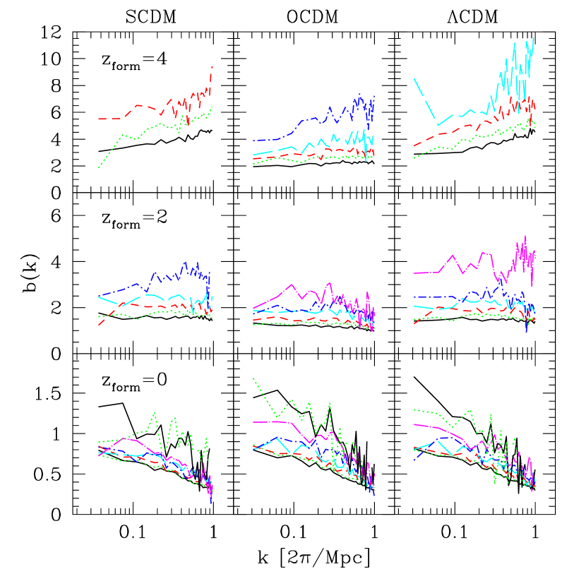
Figure 1: The square root $b(k)$ of the ratio of the power spectra of dark matter haloes to that of the dark matter, computed at the time the haloes were identified: $z=0$, $z=2$ and $z=4$ for the top, middle and bottom rows, respectively. The different line types in each panel correspond to haloes of different mass ranges (mass bins increase in size by factors of two). The more massive haloes at a given redshift typically have larger values of $b(k)$.

We will begin our comparison with simulations by showing the ratios of the halo and dark matter power spectra. The various panels in Fig. 1 show the square root of $b^{2}(k)\equiv P_{\rm halo}(k)/P_{\rm matter}(k)$ for haloes identified at $z_{\rm form}=0$, $2$, and $4$, at which time both $P_{\rm halo}(k)$ and $P_{\rm matter}(k)$ were computed. The various line types in each panel correspond to haloes with mass in different mass ranges. The lowest mass halo we consider has twenty particles, and the mass bins increase in size by factors of two. Thus, the lower limit of the $m$th bin is at $10\times 2^{m}$ particles per halo ($m>0$). One consequence of this is that the highest redshift outputs of the GIF simulations are only able to probe high values of $b(k)$, whereas lower redshift outputs primarily probe lower values of $b(k)$.

An optimist would argue that the figure shows that $b(k)$ is approximately independent of $k$ for small $k$, though this approximation is more accurate when $b(k)\sim 1$ than otherwise. At a given redshift, the small $k$ value of $b(k)$ increases with halo mass. If the model presented in the previous section is correct, then we should be able to use the shape of the halo mass function to model this dependence accurately. We turn, therefore, to the shape of the halo mass function in the GIF simulations.

The shape of the unconditional mass function is expected to depend on the initial fluctuation distribution (e.g. Press & Schechter 1974). If the initial distribution is Gaussian with a scale free spectrum, then the unconditional mass function can be expressed in units in which it has a universal form that is independent of redshift and power spectrum. Namely, let $\nu\equiv[\delta_{\rm c}(z)/\sigma(m)]^{2}$, where $\delta_{\rm c}(z)$ is that critical value of the initial overdensity which is required for collapse at $z$, computed using the spherical collapse model, and $\sigma(m)$ is the value of the rms fluctuation in spheres which on average contain mass $m$ at the initial time, extrapolated using linear theory to $z$. For example, in models with $\Omega_{0}=1$ and $\Lambda_{0}=0$, $\delta_{\rm c}(z)=1.68647$, and $\sigma(m)\propto(1+z)^{-1}$. Then, for initially scale free spectra in models with $\Omega_{0}=1$ and $\Lambda_{0}=0$,

$$\nu\,f(\nu)\equiv m^{2}\,{n(m,z)\over\bar{\rho}}\,{{\rm d}\log m\over{\rm d}\log\nu}$$ (9)

has a universal shape (Press–Schechter 1974; Peebles 1980; Bond et al. 1991). It is not obvious that this scaling holds for more general initial power spectra, such as those of the GIF simulations.

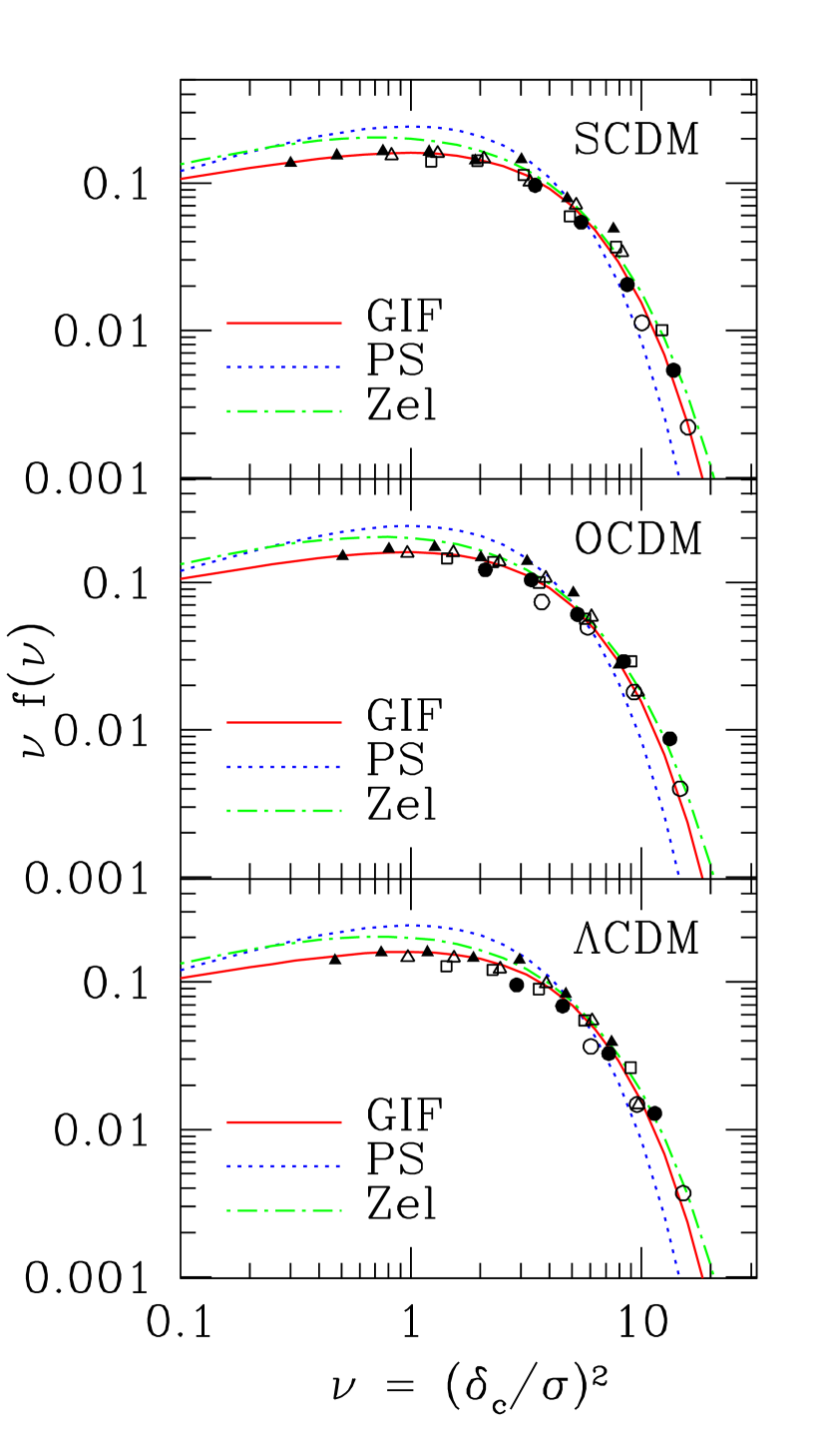
Figure 2: The unconditional mass functions from five different output times (filled triangles, open triangles, open squares, filled circles, open circles show results for $z=0$, $z=0.5$, $z=1$, $z=2$ and $z=4$) in the GIF simulations plotted as a function of the scaled variable $\nu$. Dotted curve shows the Press–Schechter prediction, dot-dashed curve shows the mass function associated with the Zeldovich approximation, and solid curve shows our modified fitting function.

The different symbols in Fig. 2 show the unconditional mass function at different output times in the GIF simulations plotted as a function of the scaled variable $\nu$. The dotted line shows the Press–Schechter formula for $\nu\,f(\nu)$; note the discrepancy at both high and low $\nu$. The dot-dashed line, which fits the data slightly better than the dashed line, is the mass function computed using the Zeldovich approximation by Lee & Shandarin (1998) (see Appendix A). The solid line through the data points shows a modification to the Press–Schechter function. It has the form:

$$\nu\,f(\nu)=A\,\left(1+{1\over\nu^{\prime p}}\right)\ \left({\nu^{\prime}\over 2}\right)^{1/2}\,{{\rm e}^{-\nu^{\prime}/2}\over\sqrt{\pi}},$$ (10)

where $\nu^{\prime}=a\,\nu$, with $a=0.707$ and $\nu=(\delta_{\rm c}/\sigma)^{2}$ as described in the previous paragraph, $p=0.3$, and $A$ is determined by requiring that the integral of $f(\nu)$ over all $\nu$ give unity. The original Press–Schechter formula has $a=1$, $p=0$, and $A=1/2$.

Recall that, in principle, the shape of $\nu\,f(\nu)$ can depend on the shape of the initial power spectrum, and on redshift. Since the different symbols in each panel overlap each other reasonably well, Fig. 2 shows that, in the GIF simulations at least, it is a good approximation to say that the mass functions scale similarly to the scale free case. So, although in principle we could have allowed $a(z,\Omega_{0},\Lambda_{0})$ and $p(z,\Omega_{0},\Lambda_{0})$ in equation (10) (in fact, we could even have allowed a different functional form for each output time of each model), Fig. 2 shows that, in practice, equation (10) with the same value of $p$ provides a reasonably good description of the mass function at all output times. This suggests that the dynamics of collapse is sensitive to $\nu$, and not to the mass scale itself. That the same value of $p$ is a good approximation to $\nu\,f(\nu)$ in all three panels is presumably a consequence of the fact that the shapes of the initial power spectra in these models are not very different. Therefore, in what follows, rather than finding best fit shapes to $\nu\,f(\nu)$ at each output time of each model, we will simply use this one function with the given constants $a$ and $p$.

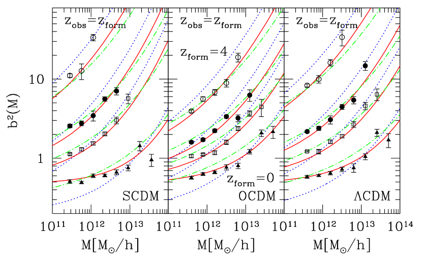
Figure 3: The large scale Eulerian bias relation at $z_{\rm obs}=z_{\rm form}$ between haloes which are identified at $z_{\rm form}$, and the mass. Solid curves show the relation we predict using the GIF mass function, dotted curves show the relations which follow from the Press–Schechter mass function, and dot-dashed curves show the relations associated with the Zeldovich mass function.

This fortuitous rescaling of the mass function is useful because it means that we need compute the peak-background split limit associated with the unconditional mass function only once, rather than having to compute it for each output time of each model. Simply set $\nu\to\nu_{10}$ in the expression above, where

$$\nu_{10}\equiv{[\delta_{\rm c}(z_{1})-\delta_{\rm c}(z_{0})]^{2}\over\sigma^{2}(m_{1})-\sigma^{2}(M_{0})}\approx{(\delta_{1}-\delta_{0})^{2}\over\sigma_{1}^{2}}\approx\nu_{1}\left(1-{2\delta_{0}\over\delta_{1}}\right),$$

with $\delta_{1}\equiv\delta_{\rm c}(\Omega_{1})$, where $\Omega_{1}\equiv\Omega(z_{1})$, $\sigma_{1}\equiv\sigma(m_{1})$ scaled using linear theory to $z_{1}$ and $\nu_{1}\equiv(\delta_{1}/\sigma_{1})^{2}$, and require that $f(m_{1}|M_{0})\,{\rm d}m_{1}=f(\nu_{10})\,{\rm d}\nu_{10}$.

Once the unconditional and conditional mass functions are known, the peak background split bias in Lagrangian space is easy to compute. It is

$$\delta^{\rm L}_{\rm h}(1|0)\approx\left[a\nu_{1}-1+{2p\over 1+(a\nu_{1})^{p}}\right]\,{\delta_{0}\over\delta_{1}}=b^{\rm GIF}_{\rm Lag}(m_{1},\delta_{1})\,\delta_{0},$$ (11)

where the final expression defines $b_{\rm Lag}^{\rm GIF}$. When $a=1$ and $p=0$ the mass function has the Press–Schechter form, and this formula reduces to the one given by Cole & Kaiser (1989) and Mo & White (1996). However, the GIF mass function has $a=0.707$ and $p=0.3$. Since $\nu_{1}$ increases with increasing halo mass, the final term in the expression above is negligible for massive haloes. In this limit, the expression above resembles the original Press–Schechter based formula, except for the factor of $a$. Since $a<1$, our formula predicts that massive haloes are slightly less biased than the original Press–Schechter based formula predicts. For less massive haloes the extra term cannot be ignored. It is positive for all $\nu_{1}$, so our formula predicts that less massive haloes are more positively biased (or less anti-biased) than the Mo & White formula suggests. The bias in Eulerian space is got by substituting this expression into equation (7):

$$b^{\rm GIF}_{\rm Eul}(m_{1},\delta_{1})=1+{a\nu_{1}-1\over\delta_{1}}+{2p/\delta_{1}\over 1+(a\nu_{1})^{p}}.$$ (12)

Both the trends discussed above remain true in Eulerian space.

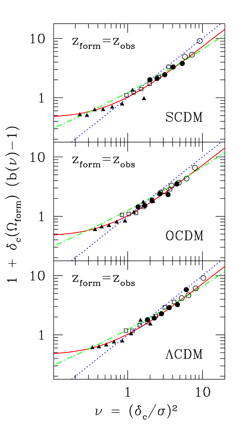
Figure 4: The large scale Eulerian bias relation of the previous figure, rescaled as indicated by the axis labels. Solid curves show the relation we predict using the GIF mass function, dot-dashed curves show the corresponding relation predicted using the Zeldovich mass function, and dotted curves show the relation which follows from the Press–Schechter mass function.

The different symbols in Fig. 3 show the large scale bias relation for haloes that are identified at $z_{\rm form}$ and are observed at $z_{\rm obs}=z_{\rm form}$. That is, they show the small $k$ values of $b^{2}(k)$ obtained as the value predicted at $k=2\pi/L$ by a linear least-square fit to the 12 left-most data points. Error bars show the formal least-square error. In this way we tried to estimate the actual large-scale bias even when $b(k)$ on the largest scales probed by the simulations shows a dependence on $k$. One might argue that the weak scale dependence of $b(k)$ in Fig. 1 means that the symbols in Fig. 3 probably slightly under/overestimate the true large scale (small $k$) value for small/large values of $b(k)$.

Each panel shows four sets of curves, corresponding to haloes which formed at $z_{\rm for}=4$, $2$, $1$, and $0$. The three curves for each redshift show how the bias relation computed using our peak background split model depends on the unconditional mass function. Solid and dotted curves show equation (12) for the GIF ($a=0.707$ and $p=0.3$) and the Press–Schechter ($a=1$, $p=0$) mass functions, respectively. The dot-dashed curves show the bias associated with the Zeldovich mass function (equation 15). As with the mass function, the dot-dashed curves fit the data better than the dotted curves, and slightly worse than the solid ones. The solid curves fit the data reasonably well for all masses and redshifts.

There are small discrepancies between our GIF based predictions and the symbols at large and small $b(M)$. Since they are in the sense discussed earlier, we suspect some of the discrepancy arises from the weak scale dependence of $b(k)$. Since these discrepancies are small, and since our measured values of $b(M)$ at small $M$ when $z=0$ are very similar to those in Fig. 3 of Jing (1998), it appears that using the ratio of the power spectra to define $b_{\rm Eul}$ gives nearly the same result as using the ratio of the correlation functions. As discussed at the end of the previous section, this is expected if the bias is independent of scale.

Suppose that the unconditional mass function $\nu\,f(\nu)$ really was independent of $z_{\rm form}$ (recall that our Fig. 2 shows this is a good approximation). Then our peak background split argument says that, after appropriate transformations, it should be possible to present the large scale bias relation as function of $\nu$ only. Namely, equation (12) suggests that we should be able to scale all the results for the different $z_{\rm form}$ above to one plot of the product ($\delta_{1}\,b_{\rm Lag}$) versus $\nu$. Fig. 4 shows the result. The symbols show the simulation data from the same output times as before. They were obtained by transforming the large scale Eulerian bias relation as indicated by the labels on the axes. The curves show the theoretical predictions for the three different mass functions we have been considering.

There are two points to be made about this plot. The first is that our peak background split model (solid curves) provides a reasonable description of the results. The main reason for including this plot is to show that the scatter about the solid curves in our plots is approximately the same as the scatter about the mass function fits in Fig. 2. As we argued above, we have no a priori reason to expect such a scaling if our relation between the unconditional mass function and the Eulerian bias were not accurate.

Finally, we can also study the case in which haloes form at high redshift, but are observed at lower redshift: $z_{\rm form}>z_{\rm obs}$. In this case, the large scale Eulerian bias should be described by our equations (7) and (12), but with

$$\nu_{1}\equiv{\delta^{2}_{\rm c}(\Omega_{\rm form})\over\sigma^{2}(m)}\qquad{\rm and}\qquad\delta_{1}\equiv{D(z_{\rm obs})\over D(z_{\rm form})}\,\delta_{\rm c}(\Omega_{\rm form})$$

where $D(z)$ is the linear theory growth factor, and $\sigma(m)$ is scaled using linear theory to its value at $z_{\rm form}$.

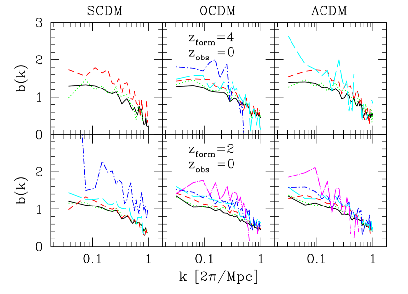
Figure 5: The square root of the ratio of the halo and matter power spectra for haloes that formed at $z_{\rm form}=4$ (top panels) and $z_{\rm form}=2$ (bottom panels) but were observed at $z_{\rm obs}=0$.

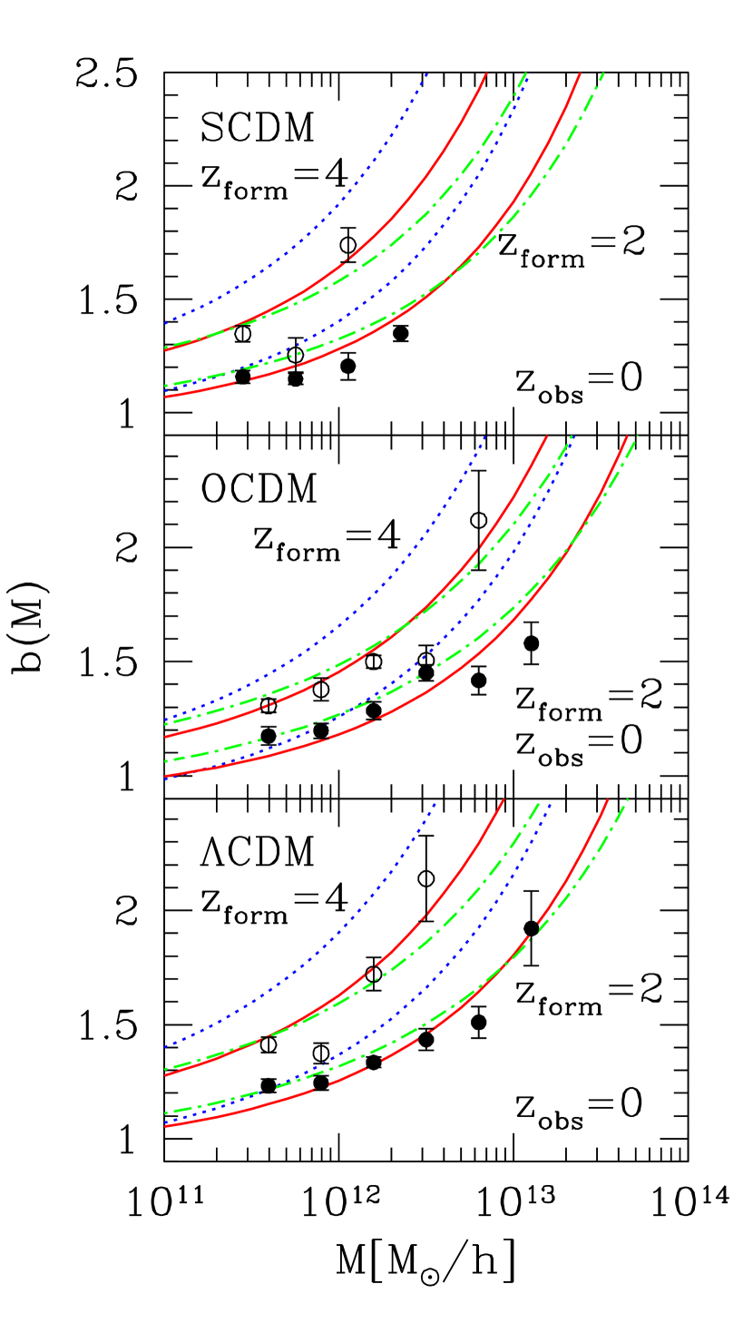
Figure 6: The large scale Eulerian bias relation at $z_{\rm obs}=0$ for haloes that formed at $z_{\rm form}$. Solid curves show the relation we predict using the GIF mass function, dotted and dot-dashed curves show the relations which follow from the Press–Schechter and Zeldovich mass functions, respectively.

Fig. 5 shows the ratio of the halo and matter power spectra for haloes which formed at $z_{\rm form}>0$ but were studied at $z_{\rm obs}=0$. Thus, it is similar to Fig. 1, except that there $z_{\rm obs}=z_{\rm form}$. There are a few obvious differences: some of the $b(k)$ curves are not particularly flat, even on the largest scales. Those curves that do asymptote nicely (at small $k$) do so at a value of $b(k)$ that is closer to unity than when $z_{\rm obs}=z_{\rm form}$. Moreover, the scale dependence of $b(k)$ is different from before: whereas previously $b(k)$ for these haloes increased with increasing $k$, now it decreases.

Estimating the large-scale value of $b(k)$ by a least-square fit as done for Fig. 3 yields the symbols shown in Fig. 6. Most of the symbols are well fit by our simple formula for the large scale bias relation. The symbols that are not well fit by our formula (typically those in the highest mass bins) almost always correspond to haloes in a mass range in which the power spectra were not particularly flat. We conclude, therefore, that our formula for the bias relation is reasonably accurate in this two epoch context as well.

4 Discussion

Collapsed haloes are biased tracers of the dark matter distribution. This bias depends on halo mass. In general, to quantify this bias requires a detailed knowledge of the merger histories of dark matter haloes. We used the peak background split to argue that, on large scales, this detailed information is unnecessary: knowledge of only the shape of the unconditional mass function is sufficient to compute a good approximation to the large scale bias relation. This fact was anticipated by Sheth & Lemson (1999), but seems to have been unnoticed before.

For example, our approach is different from, but consistent with, the recent work of Jing (1998) and Porciani, Catelan & Lacey (1998). Following Sheth & Lemson’s demonstration that the bias in Lagrangian space was not well described by standard models, Porciani et al. quantified the discrepancy. They showed that using equation (7) to transform Jing’s (1998) fitting formula for the Eulerian bias provides a reasonably good fit to the Lagrangian bias factor. In other words, their results show that equation (7) is relatively accurate. They then provided fitting functions for the Lagrangian bias relation. However, since we have argued that the Lagrangian bias is related to the halo mass function, we have chosen to provide a fit to the mass function instead.

In so doing, we showed that a simple modification (equation 10) of the Press–Schechter formula provides a good fit to the unconditional halo mass function in the SCDM, OCDM and $\Lambda$CDM models we studied (Fig. 2). This allowed us to derive a single, simple, physically motivated formula for the large scale bias relation (equation 12) that can be used for haloes of all masses at all times in all three cosmologies. Comparison of the predictions of our model with numerical simulations showed good agreement. We showed that this was true for the case in which haloes are observed at the same time as when they are first identified ($z_{\rm obs}=z_{\rm form}$), and also for the case in which haloes form at $z_{\rm form}$, evolve, and are observed at some later time $z_{\rm obs}<z_{\rm form}$.

If haloes are significantly more/less massive than the typical $M_{*}$ halo at the time of formation, then our formulae predict that they should be less/more biased than results based on the Press–Schechter formula would predict. Since galaxies are thought to form in small, i.e., $M/M_{*}(z_{\rm form})<1$, haloes (Kauffmann et al. 1998b; Baugh et al. 1998), our results are useful for galaxy formation models. The first generation of stars and high redshift quasars are thought to be associated with haloes having $M/M_{*}(z_{\rm form})\gg 1$ (Haehnelt, Natarajan & Rees 1998; Haiman & Loeb 1998), so our results (for the number density as well as the bias factor) may also be useful for studies of the reionization history of our Universe.

Although we showed how the bias relation depends on the unconditional mass function (for example, the bias relation associated with the simple Press–Schechter spherical collapse mass function is different from that associated with the Zeldovich mass function), we did not provide a derivation of the shape of the mass function itself. Since the mass function in the GIF simulations is different from those predicted by simple applications of the spherical collapse model or by the Zeldovich approximation, our model is still far from complete. We hope that our results will stimulate work aimed at rectifying this.

In this regard, we think it important to stress the following fact. Bond et al. (1991) used a random walk barrier crossing model to derive the Press–Schechter unconditional mass function from the statistics of the initial fluctuation field. In their model, the Press–Schechter mass function is associated with the first crossing distribution of a barrier of constant height. The barrier height is constant because, in the spherical collapse model, there is a critical overdensity $\delta_{\rm c}$ required for collapse, and this value is independent of the mass of the collapsed object. If this same barrier crossing model is to yield the GIF mass function, then the barrier shape must depend on mass. We have solved for this barrier shape, and are in the process of developing and testing the detailed predictions of such a moving barrier model further.

Appendix A Large scale bias and the Zeldovich approximation

The universal unconditional mass function associated with the Zeldovich approximation is given by equation (9) with

$$\nu f(\nu)=Z_{\rm a}(\nu^{\prime})+Z_{\rm b}(\nu^{\prime})+Z_{\rm c}(\nu^{\prime}),$$

where

$$Z_{\rm a}(\nu^{\prime})\!\!\! = \!\!\!{25\over 4}\sqrt{10\nu^{\prime}\over\pi}\left({5\nu^{\prime}\over 3}-{1\over 12}\right)\exp\left(-5\nu^{\prime}\over 2\right){\rm erfc}\left(\sqrt{2\nu^{\prime}}\right)$$

$$Z_{\rm b}(\nu^{\prime})\!\!\! = \!\!\!{25\over 16}\sqrt{15\nu^{\prime}\over\pi}\ \exp\left(-15\nu^{\prime}\over 4\right)\,{\rm erfc}\left(\sqrt{3\nu^{\prime}\over 4}\right)$$

$$Z_{\rm c}(\nu^{\prime})\!\!\! = \!\!\!-{125\over 12}{\sqrt{5}\over\pi}\ \nu^{\prime}\,\exp\left({-9\nu^{\prime}\over 2}\right),$$

and

$$\nu^{\prime}=\left(\lambda_{\rm c}/\delta_{\rm c}\right)^{2}\,\nu=\left(\lambda_{\rm c}/\delta_{\rm c}\right)^{2}\,(\delta_{\rm c}/\sigma)^{2}$$ (13)

(Lee & Shandarin 1998). In these variables, the mass function has two free parameters: the usual spherical collapse $\delta_{\rm c}$, and the ratio $(\lambda_{\rm c}/\delta_{\rm c})$. The dot–dashed curve in Fig. 2 shows this function with the value used by Lee & Shandarin: $\lambda_{\rm c}=0.38$.

One way to approximate the associated conditional mass function is to use the peak background split discussed in the main text. In this approximation, one simply sets

$$\nu^{\prime}={(\lambda_{\rm c1}-\lambda_{\rm c0})^{2}\over\sigma_{1}^{2}-\sigma_{0}^{2}}\approx\nu^{\prime}_{1}\,(1-\delta_{\rm c0}/\delta_{\rm c1})^{2},$$

into the expression for $f(\nu)\,{\rm d}\nu$ above. Although we have not done so here, in principle, one could also allow $\lambda_{\rm c}(z,\Omega_{0},\Lambda_{0})$. In our case, the associated Lagrangian large scale bias is given by equation (4), so

$$\delta_{\rm h}^{\rm L}(1|0) \approx {\delta_{0}\over\delta_{1}}\ \Biggl{[}5\,\nu^{\prime}_{1}-1-2\,Z_{\rm a}(\nu^{\prime}_{1})\,{20\nu^{\prime}_{1}\over 20\nu^{\prime}_{1}-1}$$ (14)

$$\qquad\qquad\qquad+{5\over 4}\,\Bigl{(}2\nu^{\prime}_{1}\,Z_{\rm b}(\nu^{\prime}_{1})-Z_{\rm c}(\nu^{\prime}_{1})\Bigr{)}\Biggr{]}$$

$$\equiv b^{\rm Zel}_{\rm Lag}(m_{1},\delta_{1})\,\delta_{0}.$$

The Eulerian space peak background split bias factor for the Zeldovich approximation is given by inserting this expression for $b_{\rm Lag}$ in equation (7):

$$b^{\rm Zel}_{\rm Eul}(m_{1},\delta_{1})=1+b^{\rm Zel}_{\rm Lag}(m_{1},\delta_{1}).$$ (15)

References

- [1] Bardeen J.M., Bond J.R., Kaiser N., Szalay A., 1986, ApJ, 304, 15
- [2] Baugh C.M., Benson A.J., Cole S., Frenk C.S., Lacey C.G., 1998, MNRAS, submitted, astro-ph/9811222
- [3] Bond J. R., Cole S., Efstathiou G., Kaiser N., 1991, ApJ, 379, 440
- [4] Catelan P., Lucchin F., Matarrese S., Porciani C., 1998, MNRAS, 297, 692
- [5] Efstathiou G., Frenk C., White S. D. M., Davis M., 1988, MNRAS, 235, 715
- [6] Haehnelt M. G., Natarajan P., Rees M. J., MNRAS, 300, 817
- [7] Haiman Z., Loeb A., 1998, astro-ph/9811395
- [8] Jing Y., 1998, ApJL, 503, L9
- [9] Kauffmann G., Colberg J.M., Diaferio A., White S.D.M., 1998a, MNRAS, submitted, astro-ph/9805283
- [10] Kauffmann G., Colberg J.M., Diaferio A., White S.D.M., 1998b, MNRAS, submitted, astro-ph/9809168
- [11] Lacey C., Cole S., 1993, MNRAS, 262, 627
- [12] Lacey C., Cole S., 1994, MNRAS, 271, 676
- [13] Lee J., Shandarin S., 1998, ApJ, 500, 14
- [14] Mo H. J., White S. D. M., 1996, MNRAS, 282, 347
- [15] Mo H. J., Jing Y., White S. D. M., 1997, MNRAS, 284, 189
- [16] Porciani C., Catelan P., Lacey C., 1998, ApJL, submitted, astro-ph/9811477
- [17] Press W., Schechter P., 1974, ApJ, 187, 425
- [18] Sheth R. K., Lemson G., 1999, MNRAS, accepted, astro-ph/9808138
- [19] Tormen G., 1998, MNRAS, 297, 648