1 Introduction

Gravitational lenses are becoming a precious mean of probing the matter distribution in the Universe. From the search of matter in the Galactic halo to the study of the large-scale structures of the Universe, the gravitational lens effects offer a unique alternative to light surveys and are now widely used. This evolution is due in particular to the use of new observation devices, such as the wide field CCD cameras.

The aim of this course is to study the effects of gravitational lenses in those different astrophysical contexts. These notes are voluntarily focused on the fundamental mechanisms and the basic concepts that are useful to describe these effects. The observational consequences will be presented in more details in these proceedings by Y. Mellier (see also his review paper 1998). Related textbooks are,

• “Gravitation” by Misner, Thorne and Wheeler (1973) for General Relativity and in particular for the presentation of the geometric optics.

• “Large-scale Structures of the Universe” by Peebles (1993) for the description of the large-scale structures of the Universe.

• “Gravitational lenses” by Schneider, Ehlers & Falco (1992) for a general (but rather mathematical) exhaustive presentation of the lens physics.

The content of these notes is the following. In the first section I describe of the basic mechanisms of gravitational lenses, techniques and approximations that are usually employed. The second section is devoted to the case of a very simple deflector, a point-like mass distribution. This corresponds to microlensing events in which the deflectors are compact objects of a fraction of a solar mass that may populate the halo of our Galaxy. The last two sections are devoted to cosmological applications. After a presentation of the geometrical quantities that are specific to cosmology, I will present the various phenomena that can be observed in this context. Finally I describe the weak lensing regime. This is a rapidly developing area that should eventually allow us to map the mass distribution in the Universe. I explore how this can be used to constrain the cosmological parameters.

2 Physical mechanisms

Figure 1.  : The geometrical relationship between the deflection angle $\theta$ and the displacement angle $\beta$.

The physical mechanisms of gravitational lenses are well known since the foundation of General Relativity. Any mass concentration is going to deflect photons that are passing by with a fraction angle per unit length, $\delta\theta/\delta s$, given by

$${\delta\vec{\theta}\over\delta s}=-2\,\vec{\nabla}_{x}{\phi\over c^{2}}$$ (1)

where the spatial derivative is taken in a plane that is orthogonal to the photon trajectory and $\phi$ is the Newtonian potential.

2.1 Born approximation and thin lens approximation

In practice, the total deflection angle is at most about an arcmin. This is the case for the most massive galaxy clusters. It implies that in the subsequent calculations it is possible to ignore the bending of the trajectories and calculate the lens effects as if the trajectories were straight lines. This is the Born approximation.

Eventually, one can do another approximation by noting that in general the deflection takes place along a very small fraction of the trajectory between the sources and the observer. One can then assume that the lens effect is instantaneous and is produced through the crossing of a plane, the lens plane. This is the thin lens approximation.

2.2 The induced displacement

The direct consequence of this bending is a displacement of the apparent position of the background objects. This apparent displacement depends on the distance of the source plane, $D_{OS}$, and on the distance between the lens plane and the source plane $D_{LS}$. More precisely we have (see Fig. 1),

$$\vec{\beta}=\vec{\alpha}-{2\over c^{2}}\,{D_{LS}\over D_{OS}\,D_{OL}}\,\vec{\nabla}_{\alpha}\left(\int{\rm d}s\ \phi(s,\alpha)\right)$$ (2)

where $\vec{\alpha}$ is the position in the image plane, $\vec{\beta}^{S}$ is the position in the source plane. The gradient is taken here with respect to the angular position (this is why a $D_{OL}$ factor appears). The total deflection is obtained by an integration along the line of sight, assuming the lens is thin. In a cosmological context the exact expressions of the angular distances are not trivial, they depend on the local curvature of the background.

3 The case of a point-like mass distribution

3.1 Multiple images and displacement field

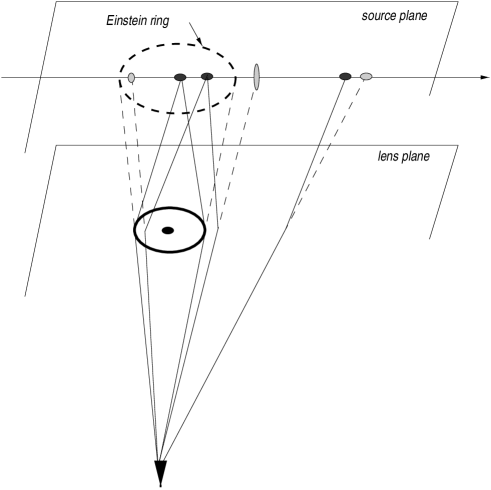
Figure 2.  : Position of the Einstein ring for a point-like mass distribution.

The potential of a point-like mass distribution is given by,

$$\phi(r)={-G\,M\over r},$$ (3)

for an object of mass $M$. Let me calculate the instantaneous deflection angle at an apparent distance $r$. We suppose that the impact parameter of the trajectory is $r$ and ${\bf x}$ is the abscissa to the point of the trajectory that is the closest to the lens (see Fig. 1). Along the trajectory the potential is given by,

$$\phi(x)={-G\,M\over\sqrt{r^{2}+x^{2}}}.$$ (4)

Then the deflecting angle is given by,

$${\delta\theta\over\delta x}=-2\,{G\,M\,r\over c^{2}\,(r^{2}+x^{2})^{3/2}}.$$ (5)

The total deflection angle $\theta$ is given by the result of the integration of this quantity with respect to $x$. It gives,

$$\theta={4\,G\,M\over r\,c^{2}}.$$ (6)

This is a well known expression which served as the first test of General Relativity with the observed displacement of stars around the solar disc (Dyson et al. 1919).

It implies that the true position of an object on the sky, $\beta$, is related to its apparent position, $\alpha$, with

$$\vec{\beta}=\vec{\alpha}-{R_{E}^{2}\over\alpha^{2}}\,\vec{\alpha}$$ (7)

where $\vec{\beta}$ and $\vec{\alpha}$ are 2D angular position vectors and $R_{E}$ is the Einstein radius,

$$R_{E}=\sqrt{{4\,G\,M\over c^{2}}\,{D_{LS}\over D_{OS}\,D_{OL}}}.$$ (8)

One can see that when $\alpha^{2}=R_{E}^{2}$ the lens and the background objects are necessarily aligned. It implies that, since the optical bench is symmetric around its axis, the observed object appears as a perfect ring (see Fig. 2). It is worth noting that for this potential, except for this particular position, all background objects have two images. This is however quite specific to a point like mass distribution which has a singular gravitational potential.

The problem is that none of these features are observable when the lens is a star. Let for example assume that we have a one solar mass star in the halo of our galaxy (therefore at a distance of about 30 $kpc$). The apparent size of such a star is about $10^{-8}$ arcsec. Its Einstein ring is about $10^{-4}$ arcsec. None of these dimensions are accessible to the observations (the angular resolution of telescope is at best a few tens of arcsec). The Einstein radius is therefore much too small to be actually seen!

Note however that these numbers show that the point-like approximation is entirely justified for a star (the Einstein ring is much more bigger that the apparent size of a star). Simple examination of the scaling in those relations shows that this would not be true for massive astrophysical objects such as galaxies or galaxy clusters.

The detection of gravitational effects due to stars should then be done by another mean: the amplification effect.

3.2 The amplification matrix

The case of circular lenses has already given us a clue: when the source is precisely aligned with the lens, the image is no more a point but a circle. One consequence is that the observed total luminosity is much larger than what would have been observed without lenses. The effect is basically due to the variations of the displacement field with respect to the apparent position. These variations induce a change of both the size and shape of the background objects. To quantify this effect one can compute the amplification matrix ${\cal A}$ which describes the linear change between the source plane and the image plane,

$${\cal A}=\left({\partial\alpha_{i}\over\partial\beta_{j}}\right).$$ (9)

Its inverse, ${\cal A}^{-1}$, is actually directly calculable in terms of the gravitational potential. It is given by the derivatives of the displacement with respect to the apparent position,

$${\cal A}^{-1}\equiv{\partial\beta_{i}\over\partial\alpha_{j}}=\delta_{ij}-2{D_{LS}\over D_{OS}\,D_{OL}}\phi_{,ij}.$$ (10)

In case of a point-like mass distribution it is easy to see that,

$${\cal A}^{-1}=\left(\delta_{ij}\left[1-{R_{E}^{2}\over\alpha^{2}}\right]+{\alpha_{i}\alpha_{j}\over\alpha^{2}}R_{E}^{2}\right).$$ (11)

The amplification effect for each image is given by the inverse of the determinant of the amplification matrix computed at the apparent position of the image. The amplification factor is usually noted $\mu$,

$$\mu=1/\det({\cal A}^{-1}).$$ (12)

In case of the point-like distribution we have (the calculation is simple at the position $\alpha_{1}=\alpha,\ \alpha_{2}=0$),

$$\mu=\left|{\alpha^{4}\over\alpha^{4}-R_{E}^{4}}\right|,$$ (13)

for each image. The total amplification effect is given by the summation of the two effects for the 2 images,

$$\mu_{\rm tot}={u^{2}+2\over u(u^{2}+4)^{1/2}}\ \ {\rm with}\ \ u={b\over R_{E}},$$ (14)

where $b$ is the impact parameter of the background object in the source plane. The amplification effect is obviously dependent on the impact parameter. If it is changing with time, this effect is detectable.

3.3 The microlensing experiments

The microlensing experiments are based on this effect. When a compact object of the halo of our galaxy reaches, because of its proper motion, the vicinity of the light path of a background star (from the SMC or the LMC) the impact parameter is changing with time and can be small enough to induce a detectable amplification (when $u$ is about unity, the amplification is about 30%). In practice one observes changes in the magnitude of the remote stars that obey specific properties,

• the time dependence of the amplification is symmetric and has a specific shape;

• the amplification effect is unique;

• the magnitude of the amplification effect is the same in all wavelengths.

The time scale of such an event is about a few days to a few month depending on the mass of the deflectors. Currently a fair number of such events have been recorded (see contribution of J. Rich, these proceedings) and constraints on the content of our halo with low massive compact objects have been put.

4 Gravitational lenses in Cosmology

The extension of the lens equations to a cosmological context raises some technical difficulties because the background in which the objects are embedded is not flat. The aim of this section is to clarify these points. However, readers that are not familiar with cosmology can jump to section 5.

The basic equations, that describe jointly the evolution of the expansion parameter and the mean density, are the following,

$$3\,\ddot{a} = -4\pi G\,\rho\,a+\Lambda\,a;$$ (15)

$$\dot{a}^{2} = {1\over a}\left[{8\pi\,G\over 3}\,\rho\,a^{3}-k\,a+{\Lambda\,a^{3}\over 3}\right].$$ (16)

where $\Lambda$ is a possible cosmological constant and $k$ a possible curvature term. The Hubble constant reads,

$$H={\dot{a}\over a}=\sqrt{{8\pi\,G\over 3}\,\rho-{k\over a^{2}}+{\Lambda\,a^{3}\over 3}}.$$ (17)

To simplify the discussions the reduced quantities are introduced,

$$\Omega={8\pi\,G\over 3\,H^{2}}\,\rho\ \ {\rm and}\ \ \lambda={\Lambda\over 3\,H^{2}}.$$ (18)

They have an index $0$ when they are taken at present time.

4.1 The angular distances

We consider an object of size $l$ (either because of its proper size or because of a peculiar physical process) at redshift $z$. When this size $l$ is seen under an angle $\alpha$, then by definition,

$$\alpha={l\over{\cal D}_{0}},$$ (19)

where ${\cal D}_{0}$ is the angular distance. This is the distance at which this object would be in an Euclidean metric. What is then the relationship between ${\cal D}_{0}$ and $z$? The Friedmann-Robertson-Walker metric is given by,

$${\rm d}s^{2}=-c^{2}\,{\rm d}t^{2}+a^{2}(t)\left({{\rm d}x^{2}\over 1-k\,x^{2}}+x^{2}{\rm d}\theta^{2}+x^{2}\,\sin^{2}\theta\,{\rm d}\varphi^{2}\right).$$ (20)

The fact that the size of this object is $l$ means that it takes a time interval ${\rm d}t=l/c$ for light to travel to one end to the other. The corresponding angle $\alpha={\rm d}\theta$ can be obtained by writing ${\rm d}s=0$ with ${\rm d}x=0,{\rm d}\varphi=0$, which gives

$$l=a(t)\,x\,\alpha.$$ (21)

The angular comoving distance is thus given by ${\cal D}_{0}(z)=x(z)$. The expression of $x(z)$ can then be computed by the relation ${\rm d}s=0$ along the line of sight with ${\rm d}\theta=0$ and ${\rm d}\varphi=0$,

$$\int_{t_{0}}^{t_{1}}{c\,{\rm d}t\over a}=\int_{0}^{x(z)}{{\rm d}x\over\sqrt{1-kx^{2}}}\equiv\chi(z).$$ (22)

For an open Universe, $k<0$, and we have,

$$x(z)={\cal D}_{0}(z)={1\over\sqrt{-k}}\sinh[\sqrt{-k}\ \chi(z)].$$ (23)

Obviously when $k=0$, $x=\chi$.

The relation $\chi(z)$ depends on the function $a(t)$ for a given cosmology, and therefore on the matter content of the Universe, on $\Lambda$ and $k$ . For instance, for an Einstein-de Sitter Universe, in the matter dominated era, we have

$$a(t)=\left({t\over t_{0}}\right)^{2/3},$$ (24)

so that,

$$x(z)=\int_{t_{0}}^{t_{1}}t^{-2/3}{\rm d}t=3(t_{0}^{1/3}-t_{1}^{1/3})t_{0}^{2/3},\ \ H_{0}={2\over 3\,t_{0}},$$ (25)

and eventually,

$${\cal D}_{0}(z)=\chi(z)={c\over H_{0}}\left(2-{2\over\sqrt{1+z}}\right).$$ (26)

This is the comoving angular distance for an Einstein-de Sitter Universe. More generally we have an explicit solution if $\Lambda=0$ only. Finally the lens equation also requires the angular distance between two different redshifts $z_{1}$ and $z_{2}$. The calculation is actually quite simple. This distance is given formally by ${\cal D}_{0}(z_{2})$ when it is calculated at a time when the observer is at redshift $z_{1}$. $k$ being time independent we should formally have,

$${\cal D}_{0}(z_{1},z_{2})={1\over\sqrt{-k}}\sinh[\sqrt{-k}\ (\chi(z_{2},z_{1}))],$$ (27)

and to compute $\chi(z_{2},z_{1})$ one only needs to remark,

$$\chi(z_{2},z_{1})\equiv\int_{t_{1}}^{t_{2}}{c\,{\rm d}t\over a}=\chi(z_{2})-\chi(z_{1}),$$ (28)

which gives the expression of the angular distance we need. Eventually, it is fruitful to notice that,

$${c\,{\rm d}t\over a}=-{c\,{\rm d}z\over H},$$ (29)

which gives,

$${\cal D}_{0}(z_{1},z_{2})={c\over H_{0}\sqrt{1-\Omega_{0}-\lambda_{0}}}\sinh\left[H_{0}\sqrt{1-\Omega_{0}-\lambda_{0}}\ \int_{z_{1}}^{z_{2}}{{\rm d}z\over H(z)}\right],$$ (30)

and

$${\cal D}_{0}(z)={c\over H_{0}\sqrt{1-\Omega_{0}-\lambda_{0}}}\sinh\left[H_{0}\sqrt{1-\Omega_{0}-\lambda_{0}}\ \int_{0}^{z}{{\rm d}z^{\prime}\over H(z^{\prime})}\right].$$ (31)

The whole geometrical part of the lens equation is thus established.

4.2 Geometric optics in a weakly inhomogeneous Universe

What is now the source term for the deflection angle? We should first notice that in absence of lenses the light rays follow the geodesics of the Friedmann-Robertson-Walker metric. And in the applications we are interested in, the metric fluctuations are always weak. These fluctuations are given by, ${G\,M/(R\,c^{2})}$. For instance, for

• 1 star: $M=1\,M_{\odot},\ R=7\,10^{5}{\rm km},\ \delta\phi\approx 10^{-6}$;

• 1 galaxy cluster: $M=10^{15}\,M_{\odot},\ R=1{\rm Mpc}=3\,10^{19}{\rm km},\ \delta\phi\approx 10^{-5}$.

The metric inhomogeneities are thus always extremely weak, even in the most extreme cosmological situations.

Figure 3.  : Sketch showing the geometrical quantities that appear in Eq. 32

Following Sachs (1961), we consider two nearby geodesics, ${\cal L}$ and ${\cal L^{\prime}}$, in a light bundle in an FRW Universe with small metric fluctuations. We denote $\alpha_{i}$ the bi-dimensional angular distance between ${\cal L}$ and ${\cal L^{\prime}}$ as it is seen by the observer. This is the distance in the image plane, that is the difference between the angular coordinates with which the photons arrive. We denote $\xi_{i}(z)$ the real distance between ${\cal L}$ and ${\cal L^{\prime}}$ at redshift $z$ (see Fig. 3). It implies that the geodesics are straight enough so that light always travels towards the observer. We also assume that the deflections are small enough so that it is possible to make the small angle approximation,

$$\xi_{i}(z)=a\ {\cal D}_{ij}(z)\ \alpha_{j},$$ (32)

that is that we assume the the position vector $\xi_{i}$ can be obtained by a simple linear transform of the angular coordinates. For an homogeneous space ${\cal D}_{ij}(z)$ is simply given by ${\cal D}_{0}(z)\ \delta^{K}_{ij}$ where $\delta^{K}_{ij}$ is the Kronecker symbol. Obviously ${\cal D}_{ij}$ changes as a function of redshift along the trajectories. The “virtual” angular position in the source plane is then given by the ratio of the real distance (at time of light emission for instance) by the angular distance of the emitter in an homogeneous space,

$$\vec{\beta}={\vec{\xi}(z)\over a{\cal D}_{0}(z)}.$$ (33)

The amplification matrix, or rather its inverse, ${\cal A}^{-1}$, is then given by,

$${\cal A}^{-1}(z)={{\cal D}_{ij}(z)\over a{\cal D}_{0}(z)}.$$ (34)

for a source plane at redshift $z$.

Sachs (1961) gave the master equation which governs the evolution of the distance between the geodesics. The derivation of this equation goes beyond these lecture notes and I give only the final answer (as it has been given by Seitz, Schneider and Ehlers 1994),

$${{\rm d}^{2}[a\ {\cal D}_{ij}(\vec{\beta},z)]\over{\rm d}\eta^{2}}=a(z){\cal R}_{ik}(\vec{\beta},z)\ {\cal D}_{kj}(\vec{\beta},z)$$ (35)

where the derivatives are taken with respect to $\eta$,

$${\rm d}\eta=-{{\rm d}a\over H(a)}=-a\ {\rm d}t,\ \ \ \eta(z=0)=0.$$ (36)

with the boundary conditions,

$$\left({\cal D}_{ij}\right)_{z=0}=0;\ \ \left({{\rm d}{\cal D}_{ij}\over{\rm d}\eta}\right)_{z=0}={c\over H_{0}}.$$ (37)

The matrix ${\cal R}_{ij}$ represents the tidal effects. It can by written in terms of the gravitational potential $\phi$ given by,

$$\Delta_{x}\phi=4\pi\,G\,\overline{\rho}\,a^{2}\,\delta_{\rm mass}.$$ (38)

The Laplacian is taken with respect of the comoving angular distances. We have

$${\cal R}_{ij}=-{4\pi\,G\,\overline{\rho}\over H_{0}^{2}\,a^{2}}\left(\begin{array}[]{cc}1&0\\ 0&1\end{array}\right)-{2\over H_{0}^{2}\,a^{2}}\left(\begin{array}[]{cc}\phi_{,11}&\phi_{,12}\\ \phi_{,21}&\phi_{,22}\end{array}\right).$$ (39)

Since $8\pi\,G\,\overline{\rho}\,a^{3}=3H_{0}^{2}\,\Omega_{0}$, (e.g. Eq. 18) for an homogeneous Universe we have,

$${\cal R}_{ij}^{(0)}=-{3\over 2}\,(1+z)^{5}\,\Omega_{0}\,\delta^{K}_{ij}$$ (40)

(the superscript (0) means here that it is the value of ${\cal R}$ without perturbations). In this case the matrix ${\cal D}_{ij}$ is proportional to $\delta^{K}_{ij}$ and we have,

$${{\rm d}^{2}[a\ {\cal D}_{0}(z)]\over{\rm d}\eta^{2}}=-{3\over 2}(1+z)^{4}\,\Omega_{0}\,{\cal D}_{0}(z).$$ (41)

We recover in fact the comoving angular distance the expression of which we know,

$${\cal D}_{0}(z)={c\over H_{0}\sqrt{1-\Omega_{0}-\lambda_{0}}}\,\sinh\left[\sqrt{1-\Omega_{0}-\lambda_{0}}\int_{0}^{z}{{\rm d}z^{\prime}\over E(z^{\prime})}\right],$$ (42)

with

$$E(z)={H(z)\over H_{0}}=\sqrt{\lambda_{0}+(1+z)^{2}(1-\Omega_{0}-\lambda_{0})+(1+z)^{3}\Omega_{0}}.$$ (43)

This integral has a closed form only when the cosmological constant, $\Lambda$, is zero.

4.3 The linearized equation of geometric optics

We can remark that the equation (35) is not linear since ${\cal D}$ is not simply proportional to ${\cal R}$. This expresses the fact that the deformation of the angular distance is made all along the light trajectory by multiple deflections. The general resolution of Eq. (35) is in general very complicated. It can however handled when it is linearized. Let’s assume we can expand ${\cal D}_{ij}$ with respect of the local density contrast,

$${\cal D}_{ij}(z)={\cal D}_{0}+{\cal D}_{ij}^{(1)}+\dots$$ (44)

It implies that, at first order,

$${{\rm d}^{2}[a\ {\cal D}^{(1)}_{ij}(\vec{\beta},z)]\over{\rm d}\eta^{2}}-a(z){\cal R}_{ik}^{(0)}(\vec{\beta},z){\cal D}_{kj}^{(1)}(\vec{\beta},z)=-{3}\Omega_{0}(1+z)^{4}{\cal D}_{0}(z)\varphi_{,ij}(\vec{\beta},z)$$ (45)

with,

$$\left({\cal D}_{ij}^{(1)}\right)_{z=0}=0,\ \ \left({{\rm d}{\cal D}_{ij}^{(1)}\over{\rm d}\eta}\right)_{z=0}=0,$$ (46)

and we define the field $\varphi$ so that,

$$\Delta_{x}\varphi=\delta_{\rm mass}(\vec{\beta},z)={\Delta_{x}\phi\over 4\pi\,G\,\overline{\rho}\,a^{2}}.$$ (47)

To solve this differential equation it is easier to write it with the variable $z$. It then reads,

$${{\rm d}^{2}[a\ {\cal D}^{(1)}_{ij}(\vec{\beta},z)]\over{\rm d}z^{2}}+{1\over E(z)}{{\rm d}E(z)\over{\rm d}z}{{\rm d}{\cal D}^{(1)}_{ij}(\vec{\beta},z)\over{\rm d}z}-$$

$$-{1\over 1+z}{1\over E(z)}{{\rm d}E(z)\over{\rm d}z}{\cal D}^{(1)}_{ij}(\vec{\beta},z)+{3\over 2}{\Omega_{0}(1+z)\over E^{2}(z)}{\cal D}^{(1)}_{ij}(\vec{\beta},z)=$$

$$-{3}{\Omega_{0}(1+z)\over E^{2}(z)}{\cal D}_{0}(\vec{\beta},z)\varphi_{,ij}(\vec{\beta},z).$$ (48)

The differential homogeneous equation it is associated with has two known solutions. One describes the angular distance ${\cal D}_{0}$, the other is given by,

$${\cal U}_{0}(z)={1\over\sqrt{1-\Omega_{0}-\lambda_{0}}}\,\cosh\left[\sqrt{1-\Omega_{0}-\lambda_{0}}\int_{0}^{z}{{\rm d}z^{\prime}\over E(z^{\prime})}\right],$$ (49)

The general solution of 48 then reads,

$${\cal D}_{ij}^{(1)}(\vec{\beta},z)=-3\Omega_{0}\int_{0}^{z}{\rm d}z^{\prime}{(1+z^{\prime}){\cal D}_{0}(z^{\prime})\varphi_{,ij}(z^{\prime})\over E^{2}(z)}{{\cal U}_{0}(z){\cal D}_{0}(z^{\prime})-{\cal U}_{0}(z^{\prime}){\cal D}_{0}(z)\over{\cal U}_{0}^{\prime}(z^{\prime}){\cal D}_{0}(z^{\prime})-{\cal U}_{0}(z^{\prime}){\cal D}_{0}^{\prime}(z^{\prime})},$$ (50)

which, after elementary mathematical transforms, gives,

$${\cal D}_{ij}^{(1)}(\vec{\beta},z)=-3\,{\Omega_{0}}\int_{0}^{z}{{\rm d}z^{\prime}\over E(z)}{1\over\sqrt{1-\Omega_{0}-\lambda_{0}}}\times$$

$$\times\sinh\left[\sqrt{1-\Omega_{0}-\lambda_{0}}\int_{z}^{z^{\prime}}{{\rm d}z^{\prime\prime}\over E(z^{\prime\prime})}\right](1+z^{\prime}){\cal D}_{0}(z^{\prime})\varphi_{,ij}(z^{\prime}).$$ (51)

It can be rewritten by introducing the physical distance $\chi$ along the line of sight. We eventually have,

$${\cal A}^{-1}(z)={\rm Id}-{3\,\Omega_{0}\over(c/H_{0})^{2}}\int_{0}^{\chi(z)}{\rm d}\chi^{\prime}{{\cal D}_{0}(z^{\prime},z){\cal D}_{0}(z^{\prime})\over{\cal D}_{0}(z)}(1+z^{\prime})\varphi_{,ij}(z^{\prime}),$$ (52)

where the angular distances ${\cal D}_{0}(z)$ and ${\cal D}_{0}(z,z^{\prime})$ are comoving. This equation actually gives the expression of the amplification matrix for a non-trivial background. We find that the amplification matrix is given by the superposition of lens effects of the different mass layers. We can remark that the lens term is given by the gravitational potential, $\phi$, that is by the potential the source term of which is given by the density contrast.

Note finally that this equation is valid in two limit cases, either for a single lens plane with an arbitrary strength or the superposition of any number of weak lenses. This equation naturally extents the previous result, (10), obtained for a single lens in an Euclidean background. The higher orders of Eq. (35) give the intrinsic lens coupling effects (i.e. their nonlinear parts). We will not consider them here.

5 Galaxy clusters as gravitational lenses

The study of galaxy clusters has become a very active field since the discovery of the first gravitational arc by Soucail et al. (1988) in Abell cluster A370. Galaxy clusters give the most dramatic example of gravitational lens effects in a cosmological context. The difficulty is however to describe the shape of their mass distribution.

5.1 The isothermal profile

For an isothermal profile we assume that the local density $\rho(r)$ behaves like,

$$\rho(r)=\rho_{0}\left({r\over r_{0}}\right)^{-2}.$$ (53)

With such a density profile the total mass is not finite. So this is not a realistic description but it is a good starting point for the central part of clusters. It is actually more convenient to parameterize the depth of a potential well with the velocity dispersion it induces. The velocity dispersion is due to the random velocity that particles acquire when they reach a sort of thermal equilibrium. Such a dispersion is in principle measurable with the observed galaxy velocities along the line of sight. The velocity dispersion is related to the mass $M(<r)$ of the potential well that is included within a radius $r$,

$$\sigma^{2}(r)\sim{G\,M(<r)\over r}.$$ (54)

In case of a isothermal profile, the velocity dispersion is independent of the radius and we have

$$\sigma^{2}=2\pi\,G\,\rho_{0}\,r_{0}^{2}.$$ (55)

The integrated potential along the line of sight is given by,

$$\varphi(r)=2\pi\,\sigma^{2}\,r.$$ (56)

As a consequence the amplitude of the displacement is independent of the distance to the cluster center and

$$\vec{\beta}=\vec{\alpha}-{4\pi\over c^{2}}\,{D_{LS}\over D_{OS}}\sigma^{2}\,{\vec{\alpha}\over\alpha}.$$ (57)

The position of the Einstein ring is obviously given by,

$$\alpha=R_{E}={4\pi\over c^{2}}\,\,{D_{LS}\over D_{OS}}\sigma^{2},$$ (58)

which depends both on the velocity dispersion and on the angular distances. The number of images depends in this case on the value of the impact parameter. If it is too large (i.e. larger than $R_{E}$) then each background object has only one image. For a galaxy cluster of a typical velocity dispersion of $500\ km/s$, and for a source plane situated at twice the distance of the lens, the size of the Einstein ring is about $0.5$ arcmin. It is interesting to note that the size of the Einstein ring is directly proportional to the square of velocity dispersion (in units of $c^{2}$) and to the ratio $D_{LS}/D_{OS}$.

The amplification matrix reads,

$${\cal A}^{-1}=\left(\begin{array}[]{cc}1&0\\ 0&1-{1\over x}\end{array}\right),$$ (59)

where we have,

$$x={r\over R_{E}}.$$ (60)

As a result the amplification is given by,

$$\mu={x\over 1-x}.$$ (61)

Once again the amplification becomes infinite when $x\to 1$ that is, close to the critical line.

5.2 The critical lines for a spherically symmetric mass distribution

Figure 4.  : Graphical determination of the position and number of images from the shape of the potential.

The two previous cases correspond to specific profiles. In this part I only assume a spherical symmetric profile. The displacement is then given by the derivative of the potential,

$$\vec{\beta}=\vec{\alpha}-{{\rm d}\varphi\over{\rm d}r}{\vec{\alpha}\over\alpha}.$$ (62)

It is interesting to visualize this relation with a graphic representation. This is proposed in Fig. 4. The number and position of the images of a given background object are given by the number of intersection points between the curve and a straight line of slope unity. This is a direct consequence of the relation,

$$b-a=-{{\rm d}\varphi(a)\over{\rm d}a}$$ (63)

when the potential is computed along a given axis that crosses the cluster through the center and $a$ and $b$ are the abscissa on this axis of one given object in respectively the source and the image plane.

The interesting quantity is also the amplification matrix that indicates the position of the critical lines. In general this matrix reads,

$${\cal A}^{-1}=\left(\begin{array}[]{cc}1-{\partial^{2}\varphi\over\partial r^{2}}&0\\ 0&1-{1\over r}{\partial\varphi\over\partial r}\end{array}\right),$$ (64)

when it is written in the basis $(\vec{e}_{r},\vec{e}_{\theta})$. Then the amplification is infinite in two cases, when

$${\partial^{2}\varphi\over\partial r^{2}}=1\ \ {\rm or}\ \ {1\over r}{\partial\varphi\over\partial r}=1.$$ (65)

The second eigenvalue corresponds to the same case as for a singular isothermal profile. At this particular position the source forms an Einstein ring. The first eigenvalue, however, is associated with an eigenvector that is along the $x$ direction, that is along the radial direction. It means that the ”arc” which is thus formed is radial. It graphically corresponds to the case of two merging roots. It is therefore directly associated with the behavior of the potential near the origin.

5.3 The isothermal profile with a core radius

Let us consider a simple case where the projected potential is made regular near the origin,

$$\varphi(r)=\varphi_{0}\,\sqrt{1+(r/r_{c})^{2}}$$ (66)

The constant $\varphi_{0}$ is related to the velocity dispersion with

$$\varphi_{0}={4\pi\sigma^{2}\over c^{2}}\,{D_{LS}\,D_{OL}\over D_{OS}\,r_{c}}$$ (67)

where $\sigma$ is here the velocity dispersion at a radius much larger that $r_{c}$ (the velocity dispersion decreases to zero at the origin in this model). This is a more realistic case. It is interesting to note that in this case the potential is not necessarily critical (there may be no region of multiple images, see Fig. 4). When it is critical the discovery of a radial arc is an extremely precious indication for the value of the core radius.

5.4 Critical lines and caustics in realistic mass distributions

In realistic reconstructions of lens potential however, it is very rare that the lens is circular. Most of the time the mass distribution of the lens is much more complicated. It induces complex features and series of multiple images.

Figure 5.  : Shape of the caustic lines (thick lines) and critical lines (thin lines) for an elliptic potential and for different values of the central potential.

The simplest assumption beyond the spherically symmetric models is to introduce an ellipticity $\epsilon$ in the mass distribution (Kassiola & Kovner 1993),

$$\varphi={\varphi_{0}\sqrt{1+r_{\rm em}^{2}/r_{c}^{2}}}\ \ {\rm with}\ \ r_{\rm em}^{2}={x^{2}\over(1-\epsilon)^{2}}+{y^{2}\over(1+\epsilon)^{2}}.$$ (68)

To understand the physics it induces one should introduce the caustics and critical lines. The critical lines are the location on the image plane of the points of infinite magnification. The caustics are the location of these points on the source plane. These points are determined by the lines on which $\det({\cal A}^{-1})=0$. It means that arcs are along the critical lines and that they are produced by background galaxies that happen to be located on the caustics. On Fig. 5 one can see the shapes of the critical lines and caustics for different depth of the potential (68) (or equivalently for different positions of the source plane).

Eventually the reconstruction of galaxy cluster mass maps requires the use of more complicated models and it can be necessary to perform non-parametric mass reconstructions. Recent results have been obtained by AbdelSalam et al. (1997) for few clusters.

6 The weak lensing regime

In this section I consider the possibility of using the lens effects to probe the large-scale structures of the Universe. The difficulty is here that the distortion induced by the lenses can be very small. The projected potential should then be reconstructed with a statistical analysis on the deformation measured on a lot of background objects. Let me define more precisely the different regimes.

6.1 The mathematical description of the weak lensing regime

Depending on the magnitude of the lens effect, different regimes are possible:

• The strong regime is such that several light path are possible between the sources and the observer. It thus induces multiple images, and the images of background galaxies are often extremely distorted: this is the regime of the giant arcs. The one that has been investigated so far.

• The regime of arclets correspond to a case where there are no multiple images although a significant distortion of the background objects can be observed.

• The weak lensing regime corresponds to cases of modest distortion (typically a few %). Such effect cannot be detected with a single object and therefore should be measured in a statistical way, by averages over a large number of background galaxies.

In all cases the displacement field is not directly observable. In the weak lensing regime, the deformation only is measurable. For slightly extended objects such as background galaxies the deformation in shape is induced by the variations of the displacement field. It can actually be described by the amplification matrix, the components of its inverse are in general written,

$${\cal A}^{-1}=\left(\begin{array}[]{cc}1-\kappa-\gamma_{1}&-\gamma_{2}\\ -\gamma_{2}&1-\kappa+\gamma_{1}\end{array}\right),$$ (69)

taking advantage of the fact that it is a symmetric matrix. The components of this matrix are expressed in terms of the convergence, $\kappa$, (a scalar field) and the shear, $\gamma$ (a pseudo vector field) with

$$\kappa={1\over 2}\nabla^{2}\psi;\ \ \ \gamma_{1}={1\over 2}(\psi_{,11}-\psi_{,22})\ ;\ \ \ \gamma_{2}=\psi_{,12},\ \ {\rm with}\ \ \psi=2{D_{LS}\over D_{OS}\,D_{OL}}\phi.$$ (70)

The convergence describes the linear change of size and the shear describes the deformation. The consequences of such a transform can be decomposed in two aspects:

• The magnification effect. Lenses induce a change of size of the objects. As the surface brightness is not changed by this effect, the change of surface induces a direct magnification effect, $\mu$. This magnification is directly related to the determinant of ${\cal A}$ so that,

  $$\mu=\det({\cal A})=1/\left[(1-\kappa)^{2}-\gamma^{2}\right].$$ (71)

• The distortion effect. Lenses also induce a change of shape of the background objects. The eigenvalues of the matrix ${\cal A}^{-1}$ determine the direction and amplitude of such a deformation.

6.2 The magnification effect

In the weak lensing regime, the observational consequences of the magnification effect is a combination of a change the apparent area of the objects, that makes their detection easier, and their dilution (the total area is enlarged as well). The mean local number density of galaxies is then related to the slope of the galaxy counts, $\alpha$, through

$$n(\gamma)=n_{g}\,\mu^{2.5\alpha-1}\ \ {\rm with}\ \ \alpha={{\rm d}\log N\over{\rm d}m},$$ (72)

where $m$ is the apparent magnitude (in a given band) and $n_{g}$ is the mean number density of galaxies in the absence of lenses. Whether the number density of galaxies increases or decreases in magnified area thus depends on $\alpha$ and consequently on the selected population of objects.

Such an effect has been advocated (Broadhurst 1995 and Broadhurst et al. 1995) as a way to detect the lens effect. In general this method suffers from the fact that the background galaxies have intrinsic number density fluctuations. It is therefore more appropriate for mapping the mass fluctuations in galaxy clusters where the magnification effect is large enough to dominate. In galaxy clusters it is a cheap way to map the mass profiles. More sophisticated analysis allow even to have access to the cosmological constant $\Lambda$ by probing the extension of the depletion area (Fort et al. 1997, see contribution of Y. Mellier).

6.3 The galaxy shape matrices to measure the distortion field

The distortion effects change the shape of the background objects. The objects appear elongated along the eigenvalues of the amplification matrix. When background objects are only moderately extended (this excludes the case of arcs), their shapes can be described by the matrix,

$${\cal S}\equiv\displaystyle{\int{\rm d}^{2}\theta\,\theta_{i}\,\theta_{j}\,{\cal I}(\theta)}.$$ (73)

It is easy to relate the shape matrix in the source plane to the one in the image plane. This is obtained by a simple change of variable that uses the fact that the surface brightness of the objects is not changed. It implies

$${\cal S}^{S}={{\cal A}^{-1}\cdot{\cal S}^{I}\cdot{\cal A}^{-1}}.$$ (74)

By averaging over the shape matrices in the source plane, assuming the intrinsic shape fluctuations are not correlated, one can eventually get the value of ${\cal A}^{-1}/\sqrt{\det{\cal A}^{-1}}$. The combination we have access to is totally independent of the amplification factor. As a consequence, the quantity which is measurable is the reduced shear field,

$${\bf g}={\vec{\gamma}/(1-\kappa)}.$$ (75)

This quantity identifies with $\gamma$ only in the limit of very weak lensing (i.e. when $\kappa\ll 1$).

6.4 The construction of the projected mass density

The elaboration of methods for reconstructing mass maps from distortion fields is not a trivial issue. In a pioneering paper, Kaiser & Squires (1993) showed that this is indeed possible, at least in the weak lensing regime. It is indeed not too difficult to show that (in the single lens approximation),

$$\nabla\kappa=-\left(\begin{array}[]{cc}\partial_{1}&\partial_{2}\\ -\partial_{2}&\partial_{1}\end{array}\right)\cdot\left(\begin{array}[]{c}\gamma_{1}\\ \gamma_{2}\end{array}\right)$$ (76)

when $\kappa\ll 1$ and $\gamma_{i}\ll 1$. By simple Fourier transforms it is then possible to recover $\kappa$ from a distortion map.

Such a method was further extended in many ways. Bartelmann, Schneider and his collaborators (Bartelmann et al 1996, Schneider 1995, Seitz & Schneider 1995, Seitz & Schneider 1996, Seitz et al. 1998) have worked in detail on the edge effects, the possibility of having adaptive smoothing procedures, the use of maximum entropy method etc… This is particularly important when structures of different sizes and contrasts are present at the same time. Finally Kaiser (Kaiser 1995) exhibited the relation between the local convergence and the distortion field ${\bf g}$ which is valid in all regimes. This relation reads

$$\nabla\log(1-\kappa)=\left(\begin{array}[]{cc}1-g_{1}&g_{2}\\ g_{2}&1+g_{1}\end{array}\right)^{-1}\cdot\left(\begin{array}[]{cc}\partial_{1}&\partial_{2}\\ -\partial_{2}&\partial_{1}\end{array}\right)\cdot\left(\begin{array}[]{c}g_{1}\\ g_{2}\end{array}\right).$$ (77)

This is a non-linear and non-local relationship.

The first reconstruction of a mass map of a galaxy cluster has been done on MS1224 by Fahlman et al. (1994). Many other reconstructions have now been done or are under preparation (see Mellier 1998 and these proceedings).

7 The weak lensing as a probe of the Large-Scale Structures

7.1 The large-scale structures

The idea of probing the large-scale structures with gravitational effects is very attractive. The gravitational survey offers indeed a unique way of probing the mass concentrations in the Universe since, contrary to galaxy survey, it can provide us with mass maps of the Universe that are free of any bias. Its interpretations in terms of cosmological parameters would then be straightforward and independent on hypothesis on galaxy or cluster formation schemes.

The physical mechanisms are the same in the context of large-scale structures and the source for the gravitational effects is the gravitational potential $\phi$ given by Eq. (38). It is important to remember that the source term of this equation is $\overline{\rho}(t)\,\delta_{\rm mass}(t,{\bf x})$. The density contrast $\delta_{\rm mass}({\bf x})$ is usually written in terms of its Fourier transforms,

$$\delta_{\rm mass}({\bf x})=\int{{\rm d}^{3}{\bf k}\over(2\pi)^{3/2}}\,\delta_{\rm mass}({\bf k})\,D_{+}(t)\,\exp(\rm i{\bf k}.{\bf x}).$$ (78)

The density field is then entirely defined by the statistical properties of the random variables $\delta_{\rm mass}({\bf k})$. At large enough scale the field is (almost) Gaussian (at least for Gaussian initial conditions which is the case in inflationary scenarios). The amplitude of the fluctuations grows with time in linear theory in a known way $D_{+}(t)$. This function is simply proportional to the expansion factor for an Einstein-de Sitter Universe.

The variables are then entirely determined by the power spectrum $P(k)$,

$$\big{<}\delta_{\rm mass}({\bf k})\delta_{\rm mass}({\bf k}^{\prime})\big{>}=\delta_{\rm Dirac}({\bf k}+{\bf k}^{\prime})\,P(k).$$ (79)

The cosmological model is therefore completely determined by the power spectrum, $\Omega$ and $\Lambda$ as long as the the dark matter distribution is concerned.

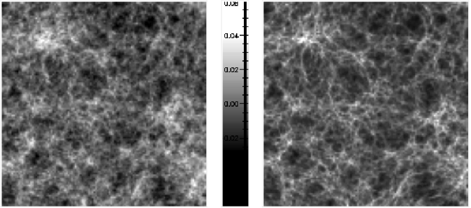
Figure 6.  : Example of reconstructions of projected mass maps. The top panels show the initial noise-free $\kappa$ map for either $\Omega=1$ (left panel) or $\Omega=0.3$ (right panel) with the same underlying linear random field and the same rms distortion. The bottom panels show the reconstructed $\kappa$ maps with noise included in the shear maps. The maps cover a total area of 25 degrees². Each pixel has an angular size of 2.5 arcmin² and averages the shear signal expected from deep CCD exposures (about 30 galaxy/arcmin²). The sources are assumed to be all at redshift unity and to have a realistic intrinsic ellipticity distribution. Such a survey is easily accessible to MEGACAM at CFHT. The precision with which the images can be reconstructed and the striking differences between the two cosmological models demonstrate the great interest such a survey would have.

7.2 The relation between the local convergence and the local density contrast

The relation between the convergence and the local density contrasts in the local universe can be derived easily from Eqs. (38, 52),

$$\kappa(\gamma)={3\over 2}\Omega_{0}\int{\rm d}z_{s}\,n(z_{s})\int{\rm d}\chi\,{{\cal D}(\chi_{s},\chi)\,{\cal D}(\chi)\over{\cal D}(\chi_{s})}\,\delta_{\rm mass}(\chi,\gamma)\,(1+z).$$ (80)

In this relation the redshift distribution of the sources in normalized so that,

$$\int{\rm d}z_{s}\,n(z_{s})=1.$$ (81)

All the distances are expressed in units of $c/H_{0}$. The relation (80) is then totally dimensionless.

7.3 The efficiency function

Figure 7.  : shape of the efficiency function, $w(z)$ (thick lines), for two different hypothesis on the shape of the redshift distribution of the sources (thin lines).

It is convenient to define the efficiency function, $w(z)$, with

$$w(z)={3\over 2}\Omega_{0}\int{\rm d}z_{s}\,n(z_{s})\,{{\cal D}(\chi_{s},\chi)\,{\cal D}(\chi)\over{\cal D}(\chi_{s})}\,(1+z)$$ (82)

On Fig. 7 one can see the shape of the efficiency function for different hypothesis for the source distribution. Obviously the further the sources are the more numerous the lenses that can be detected are, and the larger the effect is.

7.4 The amplitude of the convergence fluctuations

From this equation it is obvious that the amplitude of $\kappa$ is directly proportional of the density fluctuation amplitude and that the two point correlation function of the $\kappa$ field is related to the shape of the density power spectrum. In the following its amplitude is parameterized with $\sigma_{8}$ which is the r.m.s. of the density contrast in a sphere of radius $8\,h^{-1}$Mpc. The relation (80) also shows that $\kappa$ depends on the cosmological parameters. There is a significant dependence in the expression of the distances but the dominant contribution comes from the overall $\Omega_{0}$ factor.

The amplitude of the fluctuations of $\kappa$ depends on the angular scale at which the convergence map is filtered. We can introduce the filtered convergence $\kappa_{\theta}$, with

$$\kappa_{\theta}(\gamma)=\int{\rm d}^{2}\gamma^{\prime}\,\kappa(\gamma+\gamma^{\prime})\,W_{\theta}(\gamma^{\prime}).$$ (83)

It is convenient to introduce the Fourier transform of the window function $W(k)$. This function is,

$$W(k)=2{J_{1}(k)\over k},$$ (84)

where $J_{1}$ is the Bessel function, in case of a angular top-hat filter. Then the filtered convergence reads,

$$\kappa_{\theta}(\gamma)= \displaystyle{\int{\rm d}\chi\,w(z)\int{{\rm d}^{2}{\bf k}_{\perp}\over 2\pi}\,{{\rm d}k_{r}\over(2\pi)^{1/2}}\,\delta({\bf k})\,D_{+}(z)\,}\times$$ (85)

$$\displaystyle{\exp\left[\rm i{\bf k}_{r}\chi(z)+\rm i{\bf k}_{\perp}.\gamma{\cal D}(z0)\right]\,W\left[k_{\perp}\theta{\cal D}(z)\right]},$$

where the wave vector ${\bf k}$ has been decomposed in two parts $k_{r}$ and ${\bf k}_{\perp}$ that are respectively along the line of sight and perpendicular. The computation of the r.m.s. of $\kappa_{\theta}$ is analytic in the small angle approximation only. In such an approximation we have,

$$\theta\ll 1\ \ \Rightarrow\ \ k_{r}\ll k_{\perp}\ \ \Rightarrow\ \ P(k)\,D_{+}^{2}(z)\approx P(k_{\perp}).$$ (86)

Eventually the variance reads,

$$\big{<}\kappa^{2}_{\theta}\big{>}=\int{\rm d}\chi\,w^{2}(\chi)\,\int{{\rm d}^{2}{\bf k}\over 2\pi}\,P(k)\,W^{2}(k_{\perp}\theta{\cal D}).$$ (87)

For realistic models of the power spectrum (e.g. Baugh and Gaztañaga, 1995), the numerical result is (Bernardeau et al. 1997),

$$\big{<}\kappa^{2}_{\theta}\big{>}^{1/2}\approx 0.01\ \sigma_{8}\ \Omega_{0}^{0.8}\ z_{s}^{0.75}\ \left({\theta\over 1\deg}\right)^{-(n+2)/2}.$$ (88)

To be noticed is the dependence on the redshift of the sources. This was noticed by Villumsen (1996) who pointed out that the $\Omega_{0}$ dependence is roughly given by the $\Omega$ value at the redshift of the sources. These results are slightly affected by the introduction of the non-linear effects in the shape of the power spectrum (Miralda-Escudé 1991, Jain & Seljak 1997).

7.5 The expected signal to noise ratio

Are the effects from large-scale structures measurable? It depends on the number density of background objects for which the shape matrices are measurable. In current deep galaxy survey the typical mean number density of objects is about 50 arcmin^-2. The precision of the measured distortion at the degree scale is then about,

$$\Delta_{\rm noise}\kappa={0.3\over\sqrt{50\ 60^{2}}}\approx 10^{-3},$$ (89)

for an intrinsic ellipticity of sources of about $0.3$. This number is to be compared with the expected amplitude of the signal coming from the large-scale structures, about 1% according to Eq. (88) (see also earlier computations by Blandford et al. 1991, Miralda-Escudé 1991, Kaiser 1992). This makes such detection a priori possible with a signal to noise ratio around 10 (provided the instrumental noise can be controlled down to such a low level).

7.6 Separate measurements of $\Omega$ and $\sigma_{8}$

In Eq. (88) one can see that the amplitude of the fluctuations depend both on $\sigma_{8}$ and on $\Omega_{0}$. A question that then arises is whether it is possible to separate the amplitude of the power spectrum from the cosmological parameters. A simple examination of the equation (80) shows that it should be the case, because, for a given value of $\sigma_{\kappa}$, the density field is more strongly evolved into the non-linear regime when $\Omega_{0}$ is low.

Figure 8.  : Perturbation Theory results (Bernardeau et al. 1997) obtained for the width (left panels) and skewness (right panels) of the probability distribution function of the local convergence. The results are plotted as a function of the angular scale in the top panels, of $\Omega_{0}$ in the middle ones. The solid lines correspond to source redshifts of 1, and the dashed lines to redshifts of 2. In the bottom panels the iso-values of the width and the skewness are plotted in the $\Omega_{0}$-$\Lambda$ plane (for source redshifts of 1). It shows that the dependence on $\Omega_{0}$ is slightly degenerate with $\Lambda$.

The consequences of this are two fold. The nonlinearities change the angular scale at which the non-linear dynamics starts to amplify the growth of structures. This effect was more particularly investigated by Jain & Seljak (1997) who showed that the emergence of the nonlinear regime is apparent in the shape of the angular two-point function. This effect is however quite subtle since it might reveal difficult to separate from peculiarities in the shape of the initial power spectrum.

The other aspect is that nonlinear effects induce non-Gaussian features due to mode couplings. These effects have been studied extensively in Perturbation Theory. Technically one can write the local density contrast as an expansion with respect to the initial density fluctuations,

$$\delta_{\rm mass}({\bf x})=\delta_{\rm mass}^{(1)}({\bf x})+\delta_{\rm mass}^{(2)}({\bf x})+\dots$$ (90)

where $\delta_{\rm mass}^{(1)}({\bf x})$ is proportional to the initial density field (this is the term we have considered so far), $\delta_{\rm mass}^{(2)}({\bf x})$ is quadratic, etc. Second order perturbation theory provides us with the expression of $\delta_{\rm mass}^{(2)}({\bf x})$ (there are many references for the perturbation theory calculations, Peebles 1980, Fry 1984, Goroff et al. 1986, Bouchet et al. 1993 for the $\Omega$ dependence of this result),

$$\delta_{\rm mass}^{(2)}(t,{\bf x})= \displaystyle{\int{{\rm d}^{3}{\bf k}_{1}\over(2\pi)^{3/2}}\,{{\rm d}^{3}{\bf k}_{2}\over(2\pi)^{3/2}}\,D_{+}^{2}(t)\,\delta_{\rm lin.}({\bf k}_{1})\delta_{\rm lin.}({\bf k}_{2})\,\exp[\rm i({\bf k}_{1}+{\bf k}_{2})\cdot{\bf x}]}\times$$ (91)

$$\displaystyle{\left[{5\over 7}+{{\bf k}_{1}\cdot{\bf k}_{2}\over k_{1}^{2}}+{2\over 7}{({\bf k}_{1}\cdot{\bf k}_{2})^{2}\over k_{1}^{2}\,k_{2}^{2}}\right]},$$

where $\delta_{\rm lin.}({\bf k})$ are the Fourier components of the linear density field. It behaves essentially as the square of the linear term, with a non-trivial geometric function that contains the non-local effects of gravity.

Equivalently it is possible to expand the local convergence in terms of the initial density field,

$$\kappa(\gamma)=\kappa^{(1)}(\gamma)+\kappa^{(2)}(\gamma)+\dots$$ (92)

The apparition of a non-zero $\kappa^{(2)}$ induces non-Gaussian effects that can be revealed for instance by the computation of the skewness, third moment, of $\kappa_{\theta}$ (Bernardeau et al. 1997),

$$\big{<}\kappa_{\theta}^{3}\big{>}=\big{<}\left(\kappa_{\theta}^{(1)}\right)^{3}\big{>}+3\,\big{<}\left(\kappa_{\theta}^{(1)}\right)^{2}\kappa_{\theta}^{(2)}\big{>}+\dots$$ (93)

The actual dominant term of this expansion is $3\,\big{<}\left(\kappa^{(1)}\right)^{2}\kappa^{(2)}\big{>}$ since the first term vanishes for Gaussian initial conditions. For the computation of such term one should plug in Eq. (80) the expression of $\delta_{\rm mass}^{(2)}$ in Eq. (91) and do the computations in the small angle approximation (and using specific properties of the angular top-hat window function, Bernardeau 1995).

Eventually perturbation theory gives the following result for a realistic power spectrum (Bernardeau et al. 1997),

$$s_{3}(\theta)\equiv{\big{<}\kappa^{3}_{\theta}\big{>}\over\big{<}\kappa^{2}_{\theta}\big{>}^{2}}=40\ \Omega_{0}^{-0.8}\ z_{s}^{-1.35}.$$ (94)

The origin of this skewness is relatively simple to understand: as the density field enters the non-linear regime the large mass concentrations tend to acquire a large density contrast in a small volume. This induces rare occurrences of large negative convergences. The under-dense regions tend on the other hand to occupy a large fraction of the volume, but can induce only moderate positive convergences. This mechanism is clearly visible on the maps of figure (6). When the mean source redshift grows the skewness diminishes since the addition of independent layers of large-scale structures tend to dilute the non-Gaussianity.

Figure 9.  : Histograms of the values of $s_{3}$, top-hat filter, for $\Omega=1$ and $\Omega=0.3$ for a $5\times 5$ degree survey (thick lines) and a $10\times 10$ degree survey (thin lines).

What the Eq. (94) demonstrates is that distortion maps can be used to determine the cosmic density parameter, $\Omega_{0}$, provided the redshift distribution of the sources is well known. The hierarchy exhibited in this relation is also a direct consequence of the hypothesis of Gaussian initial conditions. Such a hierarchy has been observed for instance in galaxy catalogues (see Bouchet et al. 1993 for results in the IRAS galaxy survey). It can be very effective in excluding models with non-Gaussian initial conditions (see the attempt of Gaztañaga & Mähönen 1996). To be more precise I present the actual histograms of the measured skewness in numerical simulations (Fig. 9) which clearly demonstrate that the two cosmologies are easily separated. One can see that the scatter in $s_{3}$ is roughly the same in the two cases and that the difference in the relative precision is due to the differences in the expectation values.

The validity of Eq. (94) has been confirmed numerically by Gaztañaga & Bernardeau (1998), who showed it is valid for scales above a few tens of arcmins. A non-zero skewness has also been observed in the numerical experiment of Jain et al. (private communication, in preparation) and van Waerbeke et al. (1998). Large angular convergence maps can therefore provide new means for constraining fundamental cosmological parameters. Numerical results show that in maps of $5\times 5$ square degrees it is reasonable to expect a precision of a few percent on the normalization and about $5\%$ to $10\%$ on the cosmological density parameter depending on the underlying cosmological scenario (see Fig. 10).

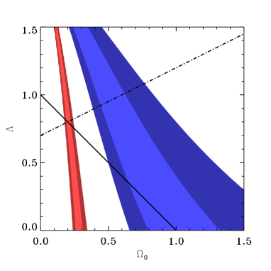
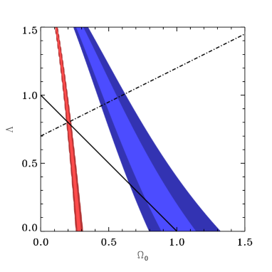
Figure 10.  : Constraints that can be brought by weak lensing survey in an $\Omega_{0}-\Lambda$ plane. The grey bands are the location of the 1 and 2-$\sigma$ locations (respectively darker and lighter bands) allowed by a measured skewness that would be obtained with either $\Omega_{0}=0.3$ (left bands) or $\Omega_{0}=1$ (right bands). The solid straight lines corresponds to a zero curvature universe, and the dot-dashed lines to a fixed acceleration parameter, $q_{0}$. The panels correspond to survey of either $5\times 5$ (top) or $10\times 10$ degrees (bottom).

7.7 Prospects

From an observational point of view, the investigation of the large-scale structures of the Universe with gravitational lenses is in a very preliminary stage. After an early claim by Villumsen (1995), a direct evidence of the detection distortion signal of gravitational origin has been reported recently by Schneider et al (1997).

There are at present many studies, either theoretical or numerical, that aim to examine all possible systematic errors (Bonnet & Mellier 1995, Kaiser et al. 1995), to optimize the data analysis concepts (such as the pixel autocorrelation function by van Waerbeke et al. 1997) and the scientific interpretations of the resulting mass maps (Bernardeau 1998, Bernardeau et al. 1997, Seljak 1997, van Waerbeke et al. 1998). A few observational surveys are now emerging,

• the ESO key program jointly done by MPA and IAP;

• the DESCART project, part of the scientific program of the wide field CCD camera to be installed at the CFHT.