Building up the Stellar Halo of the Galaxy

Abstract

We study numerical simulations of satellite galaxy disruption in a potential resembling that of the Milky Way. Our goal is to assess whether a merger origin for the stellar halo would leave observable fossil structure in the phase-space distribution of nearby stars. We show how mixing of disrupted satellites can be quantified using a coarse-grained entropy. Although after 10 Gyr few obvious asymmetries remain in the distribution of particles in configuration space, strong correlations are still present in velocity space. We give a simple analytic description of these effects, based on a linearized treatment in action-angle variables, which shows how the kinematic and density structure of the debris stream changes with time. By applying this description we find that a single dwarf elliptical-like satellite of current luminosity $10^{8}~{}{\rm L}_{\odot}$ disrupted 10 Gyr ago from an orbit circulating in the inner halo (mean apocentre $\sim 12$ kpc) would contribute about $\sim 30$ kinematically cold streams with internal velocity dispersions below 5 ${\rm km\,s^{-1}}$  to the local stellar halo. If the whole stellar halo were built by such disrupted satellites, it should consist locally of $300-500$ such streams. Clear detection of all these structures would require a sample of a few thousand stars with 3-D velocities accurate to better than 5 ${\rm km\,s^{-1}}$. Even with velocity errors several times worse than this, the expected clumpiness should be quite evident. We apply our formalism to a group of stars detected near the North Galactic Pole, and derive an order of magnitude estimate for the initial properties of the progenitor system.

1 Introduction

There have been two different traditional views on the formation history of the Milky Way. The first model was introduced by Eggen, Lynden-Bell & Sandage (1962) to explain the kinematics of metal poor halo field stars in the solar neighbourhood. According to their view the Galaxy formed in a monolithic way, by the free fall collapse of a relatively uniform, star-forming cloud. After the system became rotationally supported, further star formation took place in a metal-enriched disk, thereby producing a correlation between kinematics and metallicity: the well-known disk-halo transition. In later studies Searle & Zinn (1978) noted the lack of an abundance gradient and a substantial spread in ages in the outer halo globular cluster system. This led them to propose an alternative picture in which our Galaxy’s stellar halo formed in a more chaotic way through merging of several protogalactic clouds. (See Freeman 1987 for a complete review).

This second model resembles more closely the view of the current cosmological theories of structure formation in the Universe. These theories postulate that structure grows through the amplification by the gravitational forces of initially small density fluctuations (Peebles 1970; White 1976; Peebles 1980, 1993). In all currently popular versions small objects are the first to collapse; they then merge forming progressively larger systems giving rise to the complex structure of galaxies and galaxy clusters we observe today. This hierarchical scenario is currently the only well-studied model which places galaxy formation in its proper cosmological context (see White 1996 for a comprehensive review). Numerical simulations of large-scale structure formation show a remarkable similarity to observational surveys (e.g. Jenkins et al. 1997, and references therein; and Efstathiou 1996 for a review). For galaxy formation, the combination of numerical and semi-analytic modelling has proved to be very powerful, despite the necessarily schematic representation of a number of processes affecting the formation of a galaxy (Katz 1992; Kauffmann, White & Guiderdoni 1993; Cole et al. 1994; Navarro & White 1994; Steinmetz & Muller 1995; Kauffmann 1996; Mo, Mao & White 1998; Somerville & Primack 1999; Steinmetz & Navarro 1999). This general framework, where structure forms bottom-up, provides the background for our work.

We are motivated, however, not only by this theoretical modelling, but also by the increasing number of observations which suggest substructure in the halo of the Galaxy (Eggen 1962; Rodgers, Harding & Sadler 1981; Rodgers & Paltoglou 1984; Ratnatunga & Freeman 1985; Sommer-Larsen & Christensen 1987; Doinidis & Beers 1989; Arnold & Gilmore 1992; Preston, Beers & Shectman 1994; Majewski, Munn & Hawley 1994; Majewski, Munn & Hawley 1996). Detections of lumpiness in the velocity distribution of halo stars are becoming increasingly convincing, and the recent discovery of the Sagittarius dwarf satellite galaxy (Ibata, Gilmore & Irwin 1994) is a dramatic confirmation that accretion and merging continue to affect the Galaxy.

There have been a number of recent studies of the accretion and disruption of satellite galaxies (Quinn, Hernquist & Fullagar 1993; Oh, Lin & Aarseth 1995; Johnston, Spergel & Hernquist 1995; Velázquez & White 1995, 1999; Sellwood, Nelson & Tremaine 1998). Much of this work has been limited to objects which remain mostly in the outer parts of the Galaxy, which may be well represented by a spherical potential plus a small perturbation due to the disk (Johnston, Hernquist & Bolte 1996; Kroupa 1997; Klessen & Kroupa 1998). In this situation simple analytic descriptions of the disruption process, of the properties of the debris, etc. are possible (Johnston 1998). However, it is questionable whether such descriptions can be applied to most of the regions probed by past or current surveys of the halo, which are quite local: in this case the influence of the disk cannot be disregarded or treated as a small perturbation.

Since formation models for the Galaxy should address the broader cosmological setting, we are naturally led to ask what should be the signatures of the different accretion events that our Galaxy may have suffered through its lifetime. Should this merging history be observable in star counts, kinematic or abundance surveys of the Galaxy? How prominent should such substructures be? How long do they survive, or equivalently, how well-mixed today are the stars which made up these progenitors? What can we say about the properties of the accreted satellites from observations of the present stellar distribution? Our own Galaxy has a very important role in constraining galaxy formation models, because we have access to 6-D information which is available for no other system. Observable structure which could strongly constrain the history of the formation of galaxies is just at hand.

This paper will try to answer some of the questions just posed. We focus on the growth of the stellar halo of the Galaxy by disruption of satellite galaxies. We have run numerical simulations of this process, and have studied the properties of the debris after many orbits, long after the disruption has taken place. We analyse how the debris phase-mixes by following the growth of its entropy and the variations of the volume it fills in coordinate space. We also study the evolution of its kinematical properties. In order to model the characteristic properties of the disrupted system, such as its size, density and velocity dispersion, we develop a simple analytic prescription based on a linearized Lagrangian treatment of its evolution in action-angle variables. We apply our results to derive the observable properties of an accreted halo in the solar neighbourhood. We also analyse the clump of halo stars detected near the NGP by Majewski et al. (1994), and obtain an order of magnitude estimate for the initial properties of the progenitor system.

Our paper is organized as follows. Section 2 presents our numerical simulations. In Section 3 we analyse the characteristics of the debris in these models, and in Section 4 we develop an analytic formalism to understand their properties. We apply this formalism to describe the characteristics of an accreted halo in this same section. In Section 5 we compare our modelling with the observations of Majewski et al. (1994). We leave for the last section the discussion of the results, their validity, and the potential of our approach for understanding the formation of our Galaxy.

2 The simulations

To study the disruption of a satellite galaxy of the Milky Way, we carry out N-body simulations in which the Galaxy is represented by a fixed, rigid potential and the satellite by a collection of particles. The self-gravity of the satellite is modelled by a monopole term as in White (1983) and Zaritsky & White (1988).

2.1 Model

The Galactic potential is represented by two components: a disk described by a Miyamoto-Nagai (1975) potential,

$$\Phi_{\rm disk}=-\frac{GM_{\rm disk}}{\sqrt{R^{2}+(a+\sqrt{z^{2}+b^{2}})^{2}}},$$ (1)

where $M_{\rm disk}=10^{11}\,{\rm M_{\odot}}$, $a=6.5\,{\rm kpc}$, $b=0.26\,{\rm kpc}$, and a dark halo with a logarithmic potential,

$$\Phi_{\rm halo}=v^{2}_{\rm halo}\ln(r^{2}+d^{2}),$$ (2)

with $d=12\,{\rm kpc}$ and $v_{\rm halo}=131.5\,{\rm km\,s^{-1}}$. This choice of the parameters gives a circular velocity at the solar radius of $210\,{\rm km\,s^{-1}}$, and of $200\,{\rm km\,s^{-1}}$ at $\sim 100$ kpc.

We have taken two different initial phase-space density distributions for our satellites: $i$) two spherically symmetric Gaussian distributions in configuration and velocity space of 1 kpc (5 kpc) width and $5-25$ ${\rm km\,s^{-1}}$(20 ${\rm km\,s^{-1}}$) velocity dispersion, corresponding to masses of $\sim 5.9\times 10^{7}-1.5\times 10^{9}\,{\rm M}_{\odot}$ ($4.7\times 10^{9}\,{\rm M}_{\odot}$); and $ii$) a Plummer profile (1911)

$$\rho(r)=\frac{\rho_{0}}{(r^{2}+r^{2}_{0})^{5/2}},$$ (3)

with $\rho_{0}=3M/4\pi r_{0}^{3}$, $M$ being the initial mass of the satellite and $r_{0}$ its scale length. In this second case, the distribution of initial velocities is generated in a self-consistent way with the density profile. For the characteristic parameters we chose $M=10^{7}-10^{9}\,{\rm M_{\odot}}$ and $r_{0}=0.53-3.0\,{\rm kpc}$, giving a one-dimensional internal velocity dispersion $\sigma_{1D}=2.9-11.3\,{\rm km\,s^{-1}}$.

The force on particle $i$ due to the self-gravity of the satellite is represented by

$${\mathbf{F}}({\mathbf{x}}_{i})=-\frac{GM_{\rm in}}{(r_{i}^{2}+\epsilon^{2})^{3/2}}{\mathbf{r}}_{i},$$ (4)

where $M_{\rm in}$ is the mass of the satellite inside $r_{i}=|{\mathbf{x}}_{i}-{\mathbf{x}}_{c}|$, ${\mathbf{x}}_{c}$ being the position of the expansion centre defined by a test particle with the same orbital properties as those of the satellite. The value for the softening $\epsilon$ is $0.25\,r_{0}$. The approximation for the self-gravity of the satellite may not be very accurate during the disruption process, where tidal forces are strong and elongations in the bound parts of the satellite are expected. However, because we are interested in what happens after many perigalactic passages, well after the satellite has been tidally destroyed, our conclusions on the whole process are unaffected by details of the disruption process.

In total we ran sixteen different simulations, six of which we analyse and describe in full detail in Section 3. Some of the remaining simulations are used in Section 4 for comparison with the analytic predictions and the rest are briefly mentioned in the discussion. The characteristic properties of our six principal simulations are summarized in Table 1. They differ only in their orbital parameters and all initially have a Plummer profile and a mass of $10^{7}\,{\rm M}_{\odot}$. We have imposed the restriction that the orbits pass close to the solar circle in order to be able to compare the results of the experiments with the known properties of the local stellar halo. In all cases the satellite was represented by $10^{5}$ particles of equal mass.

Figure 1: Projections of the orbits of the satellite on different orthogonal planes, where XY coincides with the plane of the Galaxy. All distances are in $\rm kpc$.

Table 1: 0rbital parameters for the different experiments.

Experiment	pericentre	apocentre	$z_{\rm max}$	period
	(kpc)	(kpc)	(kpc)	(Gyr)
1	10.9	51.5	25.0	0.69
2	13.5	93.1	69.1	1.23
3	5.0	51.5	5.1	0.64
4	9.2	96.5	12.0	1.24
5	0.5	45.5	30.1	0.56
6	6.0	37.0	24.8	0.48

In Figure 1 we show projections of orbits 1–6 in three orthogonal planes, where XY always coincides with the plane of the Galaxy. Notice that the plane of motion of a test particle on these orbits changes orientation substantially showing that the non-sphericity induced by the disk significantly affects the motion of the satellite.

While orbiting the Galaxy, the satellite loses all of its mass. As expected, the most dramatic effects take place during pericentric passages. The satellites do not survive very long, being disrupted completely after 3 passages. This means that for our experiments, for any relatively low density satellite on an orbit which plunges deeply into the Galaxy with a period of 1 Gyr or less, the disruption itself occupies only a relatively small part of the available evolution time.

3 Properties of the debris: Simulations

3.1 Entropy as a measure of the phase-mixing

The state of a collisionless system is completely specified by its distribution function $f({\mathbf{x}},{\mathbf{v}},t)$. In making actual measurements, it is often more useful to work with the coarse-grained distribution function $\langle\,\!f\!\,\rangle$, which is the average of $f$ over small cells in phase-space. An interesting property of the coarse-grained distribution function is that it can yield information about the degree of mixing of the system (Tremaine, Hénon & Lynden-Bell 1986; Binney and Tremaine 1987).

In statistical mechanics the entropy is defined as

$$S=-\int d^{3}x~{}d^{3}v~{}f({\mathbf{x}},{\mathbf{v}},t)\ln f({\mathbf{x}},{\mathbf{v}},t).$$ (5)

Since the coarse-grained distribution function decreases as the system evolves towards a well-mixed state, an entropy calculated using $\langle\,\!f\!\,\rangle$ will increase, whereas one calculated using $f$ will remain constant, a consequence of the collisionless Boltzmann equation: $Df/Dt=0$. We therefore quantify the mixing state of the debris by calculating its coarse-grained entropy as a function of time. We represent the coarse-grained distribution function by taking a partition in the 6-dimensional phase-space and counting how many particles fall in each 6-D box. Naturally the size chosen for the partition and the discreteness of the simulations will affect the result. We can quantify the expected discreteness noise in the following way.

The uncertainty in the entropy can be attributed to fluctuations in the number counts, which we can estimate as Poissonian, $\propto\sqrt{N_{i}}$ in each occupied cell. Therefore, the uncertainty in the entropy in each cell is

$$\Delta S_{i}\approx\frac{\Delta N_{i}}{N}\left(1+\ln\frac{N_{i}}{N}\right)\approx\frac{\sqrt{N_{i}}}{N}\ln N$$

for $N\gg 1$. The total uncertainty is thus

$$\Delta S\approx\frac{\ln N}{\sqrt{N}}$$ (6)

which, for experiments with $10^{5}$ particles is $0.04$. In order to have a normalized measure of the mixing properties of the debris, we also computed the entropy of points equidistant in time along the corresponding orbit. After a very long integration, the orbit will fill the available region in phase-space, whose shape and size are determined by its integrals of motion. In this way, by comparing the entropy calculated for the debris with the ‘entropy of the orbit’, we have a measure of how well mixed the debris is. We plot this ‘normalized’ entropy in Figure 2(a) as a function of time. Note that the orbits which have the shortest periods show the most advanced state of mixing, but that this is not complete after a Hubble time.

The degree of mixing basically depends on the range of orbital frequencies in the satellite, essentially as $(\Delta\nu)^{-1}$ (Merritt 1999). This means, for example, that a small satellite will disperse much more slowly than a larger one on the same orbit. On the other hand a satellite set close to a resonance will mix on a much longer time scale. One can also imagine that if there are fewer isolating integrals than degrees of freedom so that chaos might develop, a satellite located initially in a chaotic region will have a large spread $\Delta\nu$ because of the extreme sensitivity to the initial conditions. Therefore the mixing timescale (no longer a phase-mixing timescale) will be very short, since the neighbouring orbits diverge exponentially, instead of like power-laws. If indeed the mixing rate is set by the spread in the orbital frequencies $\nu$ of the satellite, by normalising the time variable with this timescale we should be able to derive a unique curve for the entropy evolution $S=S_{\rm max}f(t/T_{\rm mix})$.

In what follows we shall assume that the behaviour of the system is regular as seems to be the case for our experiments. Let us recall that any regular motion can be expressed as a Fourier series in three basic frequencies (Binney & Spergel 1984, Carpintero & Aguilar 1998). The motion is therefore a linear superposition of waves of the basic frequencies with different amplitudes. Terms in this expansion which have the largest amplitude will be the dominant terms and may be used to define three independent (basic) frequencies. By performing a spectral dynamics analysis as outlined by Carpintero & Aguilar (1998) for ten randomly selected particles in our satellites in each experiment, we compute the frequencies associated with the largest amplitude terms in the $x$- (or $y$, since the problem is axisymmetric) and $z$-motions, and their dispersion around the mean. We then define

$$T_{\rm mix}^{-1}=min\{\sigma(\nu_{x}^{(1)}),\sigma(\nu_{x}^{(2)}),\sigma(\nu_{z}^{(1)}),\sigma(\nu_{z}^{(2)})\},$$ (7)

The curves obtained by scaling time with $T_{\rm mix}$ are shown in Figure 2(b) and they can be well fitted with the function

$$\frac{S}{S_{\rm max}}=0.78-0.69\,\exp(-27.03\,\frac{t}{T_{\rm mix}}).$$ (8)

The good fit and small dispersion confirms that mixing is governed primarily by the spread in frequency.

3.2 Configuration space properties

To analyse the spatial properties of the debris several Gyr after disruption, we have plotted smoothed isodensity surfaces and calculated different characteristic densities. In Figures 3 and 4 we show the density surface at approximately $10^{-6}$ times the initial density of the satellite. This encompasses most of the satellite’s mass.

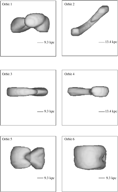
Figure 3: Isodensity surface of $10^{-6}\rho_{0}$ after 14 Gyr, seen from the Galactic plane, for the different experiments.

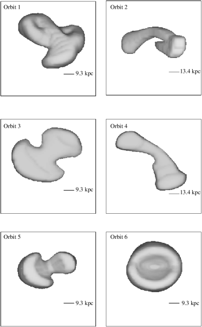
Figure 4: Isodensity surface of $10^{-6}\rho_{0}$ after 14 Gyr, seen from the Galactic pole, for the different experiments.

This density surface practically does not change over the last 2 Gyr for experiments 3, 5, 6, showing that the system has reached a stage where it fills most of its available 3-D coordinate space. The shape of this isodensity surface also gives a measure of how advanced the disruption is. The form of the accessible 3-D configuration volume is basically a torus, defined by the apocentre, pericentre and the inclination of the orbit. In Figures 3 and 4 we clearly see that shape for experiment 6. Experiments 3 and 5 are in an intermediate state and still need to fill part of their tori. In the opposite limit, experiment 2 has filled only a small fraction of its available volume. All this is consistent with what was found using the entropy in the previous subsection. The characteristic extent of the debris is much larger than the initial size of the satellite. Moreover, debris with these properties may well span a very large solid angle on the sky, and so be poorly described as a stream in coordinate space. This is the principal difference between our own experiments and those in which the Galaxy is represented by a spherical potential. In the latter the plane of motion of the satellite has a fixed orientation, and therefore all the particles have to remain fairly close to this plane, naturally giving a stream-like configuration. Late accretion events in the outer halo of the Galaxy will plausibly have this characteristic, as shown in Johnston et al. (1996) and Johnston (1998). However, similar behaviour should not be expected in the solar neighbourhood, or even as far as 10–15 kpc from the galactic centre since at such radii no strong correlations are left in the spatial distribution of satellite particles. Any method which attempts to find moving groups purely by counting stars will probably fail in this regime.

In Table 2, we present a summary of characteristic densities at different times which were calculated by counting particles within spheres of $0.5\,{\rm kpc}$ radii. The maximum density is achieved at the pericentre of the orbit, though most of the mass is distributed closer to the apocentre. In all cases the maximum density is between three and four orders of magnitude lower than the initial density of the satellite, and the mean density of the debris is between four and five orders of magnitude lower. These values give another estimate of the degree of mixing of the debris. Note that, in accordance with the entropy computation, experiment 6 has the smallest characteristic densities, meaning that it has reached a rather evolved state, whereas experiment 2 has high densities in comparison to the rest. The maximum density in all of the experiments is roughly comparable (similar or an order of magnitude lower) to the local density of the Milky Way’s stellar halo, though the sizes of regions where this density is reached get fairly small, a few ${\rm kpc}^{3}$, as the evolution proceeds.

Table 2: Characteristic densities for the different experiments.

Experiment	time	$\rho_{\rm mean}$	$\rho_{\rm max}$
	Gyr	$10^{2}{\rm M_{\odot}~{}kpc^{-3}}$	$10^{2}{\rm M_{\odot}~{}kpc^{-3}}$
1	5.0	67.0	886.2
	10.0	14.6	223.5
	12.5	7.0	152.8
	15.0	6.8	181.4
2	5.0	84.7	857.5
	10.0	26.5	376.2
	12.5	11.5	202.4
	15.0	9.7	288.4
3	5.0	41.5	437.4
	10.0	8.9	72.6
	12.5	8.7	181.4
	15.0	6.9	177.6
4	5.0	40.8	446.9
	10.0	5.9	99.3
	12.5	5.7	171.9
	15.0	5.1	156.6
5	5.0	36.4	996.9
	10.0	10.9	210.1
	12.5	6.1	183.3
	15.0	5.7	213.9
6	5.0	13.8	403.0
	10.0	4.3	82.1
	12.5	4.3	95.5
	15.0	3.4	63.0

3.3 Velocity space properties

Let us now focus on the characteristics of the debris in velocity space. We divided the 3-D coordinate space into boxes and analysed the kinematical properties of the particles inside each box. Figure 5 shows an example. The scatter diagrams indicate that there is a strong correlation between the different components of the velocity vector inside any given box. Notice also the large velocity range in each component when close to the Galactic centre. This shows that the debris can appear kinematically hot. As we shall see this results from a combination of multiple streams within a given box (clearly visible in Figure 5) and of strong gradients along each stream. At a given point on a particular stream the dispersions are usually very small.

Figure 5: Scatter plots of the different velocity components for stars in boxes of $\sim$ 3 kpc on a side at different locations for experiment 6 at 13.5 Gyr. Similar characteristics are observed in all our experiments.

4 Properties of the debris: Analytical approach

In this section we will develop an analytic formalism to understand and describe the spatial and kinematical properties of the stream. Let us recall that because the disruption of the satellite occurs very early in its history, the stars that were once part of it behave as test particles in a rigid potential for most of the evolution. One of the distinguishing properties of this ensemble of particles is that it initially had a very high density in phase-space, and by virtue of Liouville’s theorem, this is true at all times. At late times, however, this is no longer reflected by a strong concentration in configuration space. This evolution can be understood in terms of a mapping from the initial configuration to the final configuration, which we will describe by using the adiabatic invariants, namely the actions.

4.1 Action-Angle variables and Liouville’s theorem

Let $H=H({\mathbf{q}},{\mathbf{p}})$ be the (time-independent) Hamiltonian of the problem and $({\mathbf{q}},{\mathbf{p}})$ a set of canonical coordinates. We wish to transform the initial set $({\mathbf{q}},{\mathbf{p}})$ to one in which the evolution of the system is simpler, for example, where all the momenta $P_{i}$ are constant. To meet this last condition, it is sufficient to require that the new Hamiltonian be independent of the new coordinates $Q_{i}$: $H=H({\bf P})=E$. The equations of motion then become

$$\dot{Q_{i}}=\nu_{i},\qquad\dot{P_{i}}=0,$$

with solutions

$$Q_{i}=Q_{i}^{0}+\nu_{i}t,\qquad P_{i}=P_{i}^{0}.$$

The generating function that produces this transformation is known as Hamilton’s Characteristic function $W({\mathbf{q}},{\mathbf{P}})$, and satisfies the Hamilton-Jacobi partial differential equation:

$$H(q,\frac{\partial W}{\partial q})=E.$$

The solution to this equation involves $N$ constants of integration $\alpha_{i}$ (including $E$) for a system with $2N$ degrees of freedom. Therefore, the new momenta P may be chosen as functions of these $N$ constants of integration. A particularly simple situation occurs if the potential is separable in the original coordinate set $({\mathbf{q}},{\mathbf{p}})$. The characteristic function may then be expressed as $W=\sum_{i}W_{i}(q_{i},\alpha_{1}...\alpha_{N})$, and the Hamilton-Jacobi equation breaks up into a system of $N$ independent equations of the form:

$$H_{i}\left(q_{i},\frac{\partial W_{i}}{\partial q_{i}},\alpha_{1}...\alpha_{N}\right)=\alpha_{i},$$

each of which involves only one coordinate and the partial derivative of $W_{i}$ with respect to that coordinate. The transformation relations between the original and new sets of variables are

$$p_{i}=\frac{\partial W}{\partial q_{i}},\qquad Q_{i}=\frac{\partial W}{\partial P_{i}},$$

and each component of the characteristic function is given by

$$W_{i}(q_{i},\alpha_{1}..\alpha_{N})=\int dq_{i}^{\prime}\,p_{i}(q_{i}^{\prime},\alpha_{1}..\alpha_{N}).$$ (9)

(For more details, e.g. Goldstein 1953).

The actions and angle variables are a set of coordinates that describe simply the evolution of a system of particles. They are particularly useful in problems where the motion is periodic. The actions are functions of the constants $\alpha_{i}$ and are defined for a set of coordinates $({\mathbf{q}},{\mathbf{p}})$ as

$$J_{i}=\frac{1}{2\pi}\oint dq_{i}\,p_{i},$$ (10)

and their conjugate coordinates, the angles, are

$$\phi_{i}=\frac{\partial W}{\partial J_{i}}.$$ (11)

The evolution of the dynamical system thus becomes:

$$\phi_{i}\!\!\! = \!\!\!\phi_{i}^{0}+\Omega_{i}({\mathbf{J}})\,t,$$

$$J_{i}\!\!\! = \!\!\!J_{i}^{0}=constant.$$ (12)

4.1.1 The evolution of the distribution function

Let us assume that the initial distribution function of the ensemble of particles is a multivariate Gaussian in configuration and velocity space

$$f({\bf x},{\bf v},t^{0})=f_{0}\exp{\left[-\sum_{i=1}^{3}\frac{(x_{i}-\bar{x}_{i}^{0})^{2}}{2\sigma_{x}^{2}}\right]}\exp{\left[-\sum_{j=1}^{3}\frac{(v_{j}-\bar{v}_{j}^{0})^{2}}{2\sigma_{v}^{2}}\right]},$$

which we can also express using matrices as

$$f({\bf x},{\bf v},t^{0})=f_{0}\exp{\left[-\frac{1}{2}{{\bf\Delta}_{\varpi}^{0}}^{\dagger}{\bf\sigma}_{\varpi}^{0}{\bf\Delta}_{\varpi}^{0}\right]}.$$ (13)

Here $t^{0}$ denotes the initial time. ${\bf\Delta}_{\varpi}^{0}$ is a 6-dimensional vector, with three spatial and three velocity components, and ${{\bf\Delta}_{\varpi}^{0}}^{\dagger}$ is obtained by transposing ${\bf\Delta}_{\varpi}^{0}$. Explicitly ${\Delta_{\varpi}^{0}}_{i}=x_{i}-\bar{x}_{i}^{0}$ for $i=1..3$ and ${\Delta_{\varpi}^{0}}_{i}=v_{j}-\bar{v}_{j}^{0}$ for $i=j+3=4..6$ in a Cartesian coordinate system. The matrix ${\bf\sigma}_{\varpi}^{0}$ is diagonal with ${\sigma_{\varpi}^{0}}_{ii}=1/\sigma_{x}^{2}$ for i=1..3, and ${\sigma_{\varpi}^{0}}_{ii}=1/\sigma_{v}^{2}$ for i=4..6. As we shall see the matrix formulation is particularly useful to study the evolution of the distribution of particles of the system.

At the initial time, we perform a coordinate change from Cartesian to action-angle variables. Since the particles are initially strongly clustered in phase-space, a linearized transformation can be used to obtain the distribution function of the whole system in the (${\bf\phi},\,{\bf J}$) variables. We express this coordinate transformation as

$${\bf\Delta}_{\varpi}^{0}={\bf T}^{0}{\bf\Delta}_{w}^{0},\qquad\mbox{with}\qquad T_{ij}^{0}=\frac{\partial\varpi_{i}}{\partial w_{j}}\bigg{|}_{\bar{{\bf x}}^{0},{\bar{\bf v}}^{0}},$$ (14)

where ${\bf\varpi}=(\bf{x},\,\bf{v})$, $w=(\bf{\phi},\,\bf{J})$ and the elements of matrix ${\bf T}^{0}$ are evaluated at the central point of the system, around which the expansion is performed. By substituting this in Eq. (13), and by defining ${\bf\sigma}_{w}^{0}={{\bf T}^{0}}^{\dagger}{\bf\sigma}_{\varpi}^{0}{\bf T}^{0}$ the distribution function in action-angle coordinates becomes

$$f({\bf\phi},{\bf J},t^{0})=f_{0}\exp{\left[-\frac{1}{2}{{\bf\Delta}_{w}^{0}}^{\dagger}{\bf\sigma}_{w}^{0}{\bf\Delta}_{w}^{0}\right]},$$ (15)

that is, it is also a multivariate Gaussian, but with dispersions now given by $\sigma_{w}^{0}$.

The deviation of any individual orbit from the mean orbit, defined by the centre of mass or the central particle of the system, $\Delta_{w_{i}}=w_{i}-\bar{w_{i}}(t)$ may in turn be expressed in terms of the initial action-angle variables as

$$J_{i}-\bar{J}_{i}=J_{i}^{0}-\bar{J}_{i}^{0},$$ (16)

and

$$\phi_{i}-\bar{\phi}_{i}(t)=\phi_{i}^{0}-\bar{\phi}_{i}^{0}+\frac{\partial\Omega_{i}}{\partial J_{k}}\bigg{|}_{\bar{\bf J}}(J_{k}-\bar{J}_{k})\,t,$$ (17)

where we expanded the difference in the frequencies to first order in $J_{k}-\bar{J}_{k}$. Eqs. (16) and (17) can also be written as

$${\bf\Delta}_{w}(t)={\bf\Theta}^{-1}(t){\bf\Delta}_{w}^{0},$$ (18)

where ${\bf\Theta}(t)$ is the blockmatrix:

$${\bf\Theta}(t)=\left[\begin{array}[]{cc}{\bf{\cal I}_{3}}&-{\bf\Omega^{\prime}}t\\ {\bf 0}&{\bf{\cal I}_{3}}\end{array}\right].$$ (19)

${\bf{\cal I}_{3}}$ here is the identity matrix in 3-D, and ${\bf\Omega^{\prime}}$ represents a $3\times 3$ matrix whose elements are $\partial\Omega_{i}/\partial J_{j}$. The distribution function in action-angle space in the neighbourhood of the central particle at any point of its orbit $(\bar{{\bf\phi}}(t),\bar{\bf J})$ is then

$$f({\mathbf{\phi}},{\bf J},t)=f_{0}\exp{\left[-\frac{1}{2}{\bf\Delta}_{w}^{\dagger}(t){\bf\sigma}_{w}(t){\bf\Delta}_{w}(t)\right]},$$ (20)

with ${\bf\Delta}_{w}(t)=({\bf\phi}-\bar{\bf\phi}(t),{\bf J}-\bar{\bf J})$ and

$${\bf\sigma}_{w}(t)={{\bf\Theta}(t)}^{\dagger}{\bf\sigma}_{w}^{0}{\bf\Theta}(t),$$ (21)

or in terms of the original coordinates ${\bf\sigma}_{w}(t)=({\bf T}^{0}{\bf\Theta}(t))^{\dagger}{\bf\sigma}_{\varpi}^{0}({\bf T}^{0}{\bf\Theta}(t)).$

Example: 1-D Case. To understand more clearly what the distribution function in Eq. (20) tells us with respect to the evolution of the system, we consider the 1-D case. The initial distribution function becomes:

$$f(\phi,J,t^{0})=f_{0}\exp\left[-\frac{(\phi-\bar{\phi}^{0})^{2}}{2\sigma_{\phi}^{2}}-\frac{(J-\bar{J})^{2}}{2\sigma_{J}^{2}}-(\phi-\bar{\phi}^{0})(J-\bar{J})C_{\phi J}\right],$$

where $C_{\phi J}$ denotes the initial correlation between $\phi$ and $J$. After considering the time evolution of the system (as in Eq. (17)) we find

$$f(\phi,J,t)=f_{0}\exp\left[-\frac{(\phi-\bar{\phi}(t))^{2}}{2\sigma_{\phi}^{2}}-(J-\bar{J})^{2}\left(\frac{1}{2\sigma_{J}^{2}}+\frac{{\Omega^{\prime}}^{2}t^{2}}{2\sigma_{\phi}^{2}}\right)-(\phi-\bar{\phi}(t))(J-\bar{J})\left(C_{\phi,J}+\frac{{\Omega^{\prime}}t}{\sigma_{\phi}^{2}}\right)\right],$$

where $\Omega^{\prime}=d\Omega/dJ$. This means that the dispersion in the $J$-direction effectively decreases in time and the covariance between $\phi$ and $J$ increases with time. The system becomes an elongated ellipsoid in phase-space as time passes by as a consequence of the conservation of the local phase-space density. This evolution is illustrated in Figure 6.

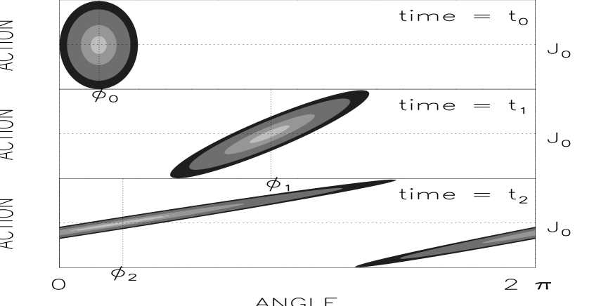
Figure 6: 1-D graphical interpretation of Liouville’s theorem and the evolution of the system in phase space. The system is initially a Gaussian in action-angle space, with no correlations between $\phi$ and $J$. As time passes by, the system evolves into an ellipsoidal configuration, with principal axes that are no longer aligned with the action or the angle directions. After a some time, the system wraps around in the angles, giving rise to phase-mixing: at the same phase we observe more than one stream, each with a small variance in the action due to the conservation of the area in phase-space.

4.1.2 The distribution function in observable coordinates

To compute the characteristic scales of a system that evolved from an initial clumpy configuration, such as satellite debris, we have to relate the dispersions in action-angle variables to dispersions in a set of observable coordinates. The transformation from the action-angle coordinate system to the observable $({\bf x},{\bf v})$ has to be performed locally since we generally cannot express in a simple way the global relation between the two sets of variables. Because the system has expanded so much along some directions in phase-space, the transformation from (${\bf\phi}$, ${\bf J}$) to $({\bf x},{\bf v})$ has to be done point to point along the orbit. This transformation is given by the inverse of ${\bf T}$ at time $t$:

$$T^{-1}_{ij}=\frac{\partial w_{i}}{\partial\varpi_{j}}\bigg{|}_{{\bf x},{\bf v}},\noindent$$ (22)

where the derivatives are now evaluated at the particular point of the orbit around which we wish to describe the system in $({\bf x},{\bf v})$ coordinates. In particular, if the expansion is performed around $(\bar{\bf\phi}(t),\bar{\bf J})$ then

$${\bf\Delta}_{w}(t)={\bf T}^{-1}{\bf\Delta}_{\varpi}(t),$$ (23)

and the distribution function may be expressed in the region around $\bar{\bf\varpi}=(\bar{\bf x},\bar{\bf v})$ as

$$f({\bf x},{\bf v},t)=f_{0}\exp{\left[-\frac{1}{2}{\bf\Delta}_{\varpi}(t)^{\dagger}{\bf\sigma}_{\bf\varpi}(t){\bf\Delta}_{\varpi}(t)\right]},$$ (24)

with

$${{\bf\Delta}_{\varpi}}_{i}(t)=\left\{\begin{array}[]{cc}x_{i}-\bar{x}_{i}(t),&i=1..3,\\ v_{j}-\bar{v}_{j}(t),&i=j+3=4..6,\end{array}\right.$$ (25)

and

$${\bf\sigma}_{\bf\varpi}(t)=({\bf T}^{0}{\bf\Theta}(t){\bf T}^{-1})^{\dagger}{\bf\sigma}_{\bf\varpi}^{0}({\bf T}^{0}{\bf\Theta}(t){\bf T}^{-1}).$$ (26)

We find once more that, locally, the distribution function is a multivariate Gaussian, where the variances and covariances depend on their initial values, on the time evolution of the system and on the position along the orbit where the system centre is located at time $t$.

If we wish to describe the properties of a group of particles that are located at a different point ${\bf\tilde{w}}$ than the central particle (i.e. the expansion centre does not coincide with the satellite centre at time $t$) a slightly different approach must be followed. The region of interest is then ${\bf\Delta}_{w}(t)=w^{\prime}-\bar{w}(t)=(w^{\prime}-{\tilde{w}})+(-\bar{w}(t)+{\tilde{w}})={\bf\Delta}^{\prime}_{w}+{\bf\tilde{D}}(t)$. We replace this in Eq. (20) and write

$$f({\bf\phi},{\bf J},t)=f_{0}\exp{\left[-\frac{1}{2}\left({\bf\Delta}^{\prime}_{w}-\tilde{\bf D}(t)\right)^{\dagger}{\bf\sigma}_{w}(t)\left({\bf\Delta}^{\prime}_{w}-\tilde{\bf D}(t)\right)\right]},$$ (27)

or equivalently

$$f({\bf\phi},{\bf J},t)=f_{0}^{\prime}(t)\exp\left[-\frac{1}{2}{{\bf\Delta}^{\prime}_{w}}^{\dagger}{\bf\sigma}_{w}(t){\bf\Delta}^{\prime}_{w}-\frac{1}{2}{{\bf\Delta}^{\prime}_{w}}^{\dagger}{\bf\sigma}_{w}(t)\tilde{\bf D}(t)-\frac{1}{2}\tilde{\bf D}(t)^{\dagger}{\bf\sigma}_{w}(t){\bf\Delta}^{\prime}_{w}\right],$$ (28)

where $f_{0}^{\prime}(t)=f_{0}\exp{[-1/2\,\tilde{\bf D}(t)^{\dagger}{\bf\sigma}_{w}(t)\tilde{\bf D}(t)]}$. We may now express ${\bf\Delta}^{\prime}_{w}={\bf T^{\prime}}^{-1}{\bf\Delta}^{\prime}_{\varpi}$, since the transformation is local again. The distribution function becomes

$$f({\bf x^{\prime}},{\bf v^{\prime}},t)=\tilde{f}_{0}(t)\exp{\left[-\frac{1}{2}({\bf\Delta}^{\prime}_{\varpi}-{\bf\delta}(t))^{\dagger}\sigma_{\bf\varpi^{\prime}}(t)({\bf\Delta}^{\prime}_{\varpi}-{\bf\delta}(t))\right]},$$ (29)

with

$${\bf\delta}(t)={\bf T}^{\prime}\tilde{\bf D}(t),\qquad\qquad{\bf\sigma}_{\bf\varpi^{\prime}}(t)=({\bf T}^{\prime-1})^{\dagger}{\bf\sigma}_{w}(t){\bf T}^{\prime-1},$$ (30)

and $\tilde{f}_{0}(t)=f_{0}^{\prime}(t)\exp{[-1/2\,({\bf T}^{-1}{\bf\delta}(t))^{\dagger}{\bf\sigma}_{w}(t){\bf T}^{-1}{\bf\delta}(t)]}$. This means that the local distribution function is Gaussian centered around ${\bf x_{m}}={\bf{\tilde{x}}}+{\bf\delta}(t)$, which in general will not be very different from ${\bf\tilde{x}}$, with variances given by the elements of ${\bf\sigma}_{\bf\varpi^{\prime}}(t)$. Thus the same type of behaviour as derived for the region around the system centre holds also if far from it.

The formalism here developed is completely general, but the actions will not always be easy to compute. As we mentioned briefly in the beginning of this section, this depends mainly on whether the potential is separable in some set of coordinates. We focus on the spherical case and a simple axisymmetric potential in the next section to show how this procedure can be used to describe the characteristic scales of the debris. We refer the reader to the Appendix for details of the computation.

4.2 Spherical Potential

4.2.1 Analytic predictions

For a spherical potential $\Phi(r)$, the Hamiltonian is separable in spherical coordinates and depends on the actions $J_{\varphi}$ and $J_{\theta}$ only through the combination $J_{\varphi}+J_{\theta}=L$. This means that the problem can be reduced to 2-D, and so we may choose a system of coordinates which coincides with the plane of motion of the satellite centre. The position of a particle is given by its angular ($\psi$) and radial ($r$) coordinates on that plane. Thus

$$L\!\!\! = \!\!\!J_{\psi}=p_{\psi},$$

$$J_{r}\!\!\! = \!\!\!\frac{1}{\pi}\int_{r_{1}}^{r_{2}}dr\frac{1}{r}\sqrt{2(E-\Phi(r))\,r^{2}-L^{2}},$$ (31)

where $L$ is the total angular momentum of the particle, $E$ its energy and $r_{1}$ and $r_{2}$ are the turning points in the radial direction of motion. The frequencies of motion and their derivatives needed to compute the matrix ${\bf\Theta}(t)$ and to obtain the time evolution of the distribution function, can be obtained by differentiating the implicit function $g=g(E,L,J_{r})\equiv 0$ defined by Eq. (4.2.1).

Let us assume that the variance matrix in action-angle variables is diagonal at $t=0$. This simplifies the algebraic computations and, since we are only trying to calculate late-time behaviour, this assumption does not have a major influence on our results. As shown in the previous section, the evolution of the system in action-angles is obtained through ${\bf\sigma}_{w}(t)={\bf\Theta}(t)^{\dagger}{\bf\sigma^{0}}_{w}{\bf\Theta}(t)$. We find the properties of the debris in configuration and velocity space by transforming the action-angle coordinates $w=(\bf{\phi},\bf{J})$ locally to the separable $\bf{\omega}=(\bf{x},\bf{p})$, and then by transforming from $\bf{\omega}=(\bf{x},\bf{p})$ to $\varpi=(\bf{x},\bf{v})$. That is ${\bf\sigma_{\varpi}}(t)={\bf T^{\prime}}^{\dagger}{\bf\sigma}_{w}(t){\bf T^{\prime}}$, with the $T^{\prime}=T_{w\rightarrow{\bf\omega}}T_{p\rightarrow v}$.

The diagonalization of the variance matrix $\sigma_{\varpi}(t)$ yields the values of the dispersions along the principal axes and their orientation. It can be shown that two of the eigenvalues increase with time, whereas the other two decrease with time. This is directly related to what happens in action-angle variables: as we have shown for the 1-D case, the system becomes considerably elongated along an axis which, after a very long time, is parallel to the angle direction. For 2-D (3-D), the evolution in action-angles can also be divided into two (three) independent motions (whether or not the Hamiltonian is separable), so that along each of these directions this same effect can be observed. The directions of expansion and contraction are linear combinations of the four axes $({\breve{\epsilon}_{\psi}},\breve{\epsilon}_{r},\breve{\epsilon}_{v_{\psi}},\breve{\epsilon}_{v_{r}})$ and, generally, none is purely spatial or a pure velocity direction.

To understand the properties of the debris in observable coordinates, we will examine what happens around a particular point in configuration space. This is equivalent to studying the velocity part of the variance matrix: $\sigma_{\varpi}(v)$. For example, by diagonalising the matrix $\sigma_{\varpi}(v)$ we obtain the principal axes of the velocity ellipsoid at the point $\bar{\bf x}$. Its eigenvalues are the roots of $\det[{\bf\sigma}_{\varpi}(v)-\lambda{\bf{\cal I}}]=0$. For $t\gg t_{\rm orb}$

$$\lambda_{1}\lambda_{2}\!\!\! = \!\!\!t^{4}\,(\Omega^{\prime}_{11}\Omega^{\prime}_{33}-{\Omega^{\prime}_{13}}^{2})^{2}r^{2}\frac{p_{r}^{2}}{\Omega_{r}^{2}}\sigma_{11}\sigma_{33},$$

$$\lambda_{1}+\lambda_{2}\!\!\! = \!\!\!t^{2}r^{2}\left[\sigma_{11}\left(\Omega^{\prime}_{11}-\frac{\Omega^{\prime}_{13}}{\Omega_{r}}\left(\Omega_{\psi}-\frac{L}{r^{2}}\right)\right)^{2}+\sigma_{33}\left(\Omega^{\prime}_{13}-\frac{\Omega^{\prime}_{33}}{\Omega_{r}}\left(\Omega_{\psi}-\frac{L}{r^{2}}\right)\right)^{2}\right]$$

$$+ t^{2}\left[\sigma_{11}{\Omega^{\prime}_{13}}^{2}+\sigma_{33}{\Omega^{\prime}_{33}}^{2}\right]\frac{p_{r}^{2}}{\Omega_{r}^{2}},$$

where the subindices 1 and 3 represent $\psi$ and $r$ respectively, and $\sigma_{ii}=1/\sigma_{\phi_{i}}^{2}$, the initial variance in the angles. Since $\sigma(v_{i})=\sqrt{1/\lambda_{i}}$ both directions in velocity space have decreasing dispersions on the average.

So far we did not describe how the debris is spread along the transverse direction to the plane of motion: $\breve{\epsilon}_{\vartheta}$ and $\breve{\epsilon}_{v_{\vartheta}}$. This is because we reduced the problem to 2-D in configuration space. However, the problem is not really 2-dimensional since the system has a finite width in the direction transverse to the plane of motion. Now that we have understood the dynamics of the reduced problem, the generalization to 3-D is straightforward. If the variance matrix initially is diagonal in action-angle variables, then the dispersions along $\phi_{\vartheta}$ and $J_{\vartheta}$ do not change because the frequency of motion in the transverse direction is zero. Thus the velocity dispersion and width of the stream also remain unchanged in the direction perpendicular to the orbital plane.

By integrating Eq. (24) with respect to the velocities, we compute the density at the point $\bar{\bf x}$

$$\rho({\bf\bar{x}},t)=\int_{\Delta v_{r}}\int_{\Delta v_{\varphi}}\int_{\Delta v_{\theta}}dv_{\theta}\,dv_{\varphi}\,dv_{r}\,f({\bf\bar{x}},{\bf v},t).$$ (32)

For $t\gg t_{\rm orb}$,

$$\rho({\bf\bar{x}},t)=\frac{(2\pi)^{3/2}f_{0}\sigma_{\phi_{3}}}{|\Omega^{\prime}_{11}\Omega^{\prime}_{33}-{\Omega^{\prime}_{13}}^{2}|}\left[\sqrt{\left(\frac{1}{\sigma_{\phi_{1}}^{2}}+\frac{1}{\sigma_{\phi_{2}}^{2}}\right)\left(\frac{1}{\sigma_{J_{1}}^{2}}+\frac{1}{\sigma_{J_{2}}^{2}}\right)}\right]^{-1}\frac{\Omega_{r}L}{r^{2}\sin\theta|p_{r}p_{\theta}|}\frac{1}{t^{2}},$$ (33)

where $\sigma_{X}$ is the initial dispersion in the quantity $X$. This equation shows that the density at the central point of the system decreases, on the average, as $1/t^{2}$. It tends to be larger near pericentre since it depends on radius as $1/r^{2}$; moreover it diverges at the turning points of the orbit. Even though the system evolves smoothly in action-angle variables, when this behaviour is projected onto observable space, singularities arise associated with the coordinate transformation. In action-angle variables the motion is unbounded, whereas in configuration space the particle finds itself at a ‘wall’ near the turning points. This divergence shows up in the elements of the transformation matrix $T_{w\rightarrow\varpi}$ (Eq. (58)), some of which tend to zero, while others diverge keeping the matrix non-singular. Because of the secular evolution of the dispersions, the intensity of the spikes will decrease with time. They are generally stronger at the pericentre of the orbit than at the apocentre, because of the $1/r^{2}$ dependence of the density.

A direct consequence of the secular evolution is that the characteristic sizes of the system, the width and length of the stream, will increase linearly with time, reflecting the conservation of the full 6-D phase-space density. At the turning points one of these scales becomes extremely small. In Figure 7 we plot the predicted behaviour of the dispersions along the principal axes of the velocity ellipsoid as a function of time. We have chosen for the initial conditions a spherically symmetric Gaussian in configuration and velocity space. We follow the evolution of the variance matrix and, in particular, of the velocity dispersions along the three principal axes at the positions of the central particle. In all panels we can clearly see the periodic behaviour associated with the orbital phase of the central particle, superposed on the secular behaviour related to the general expansion of the system along the two directions in the orbital plane. The dispersion in the third panel is on average constant: it is in the direction perpendicular to the plane of motion. Its periodic behaviour is due to the fact that we did not start with a diagonal matrix in action-angles. The initial transformation from $({\bf x},{\bf v})$ to $({\bf\phi},{\bf J})$ produces cross terms between all three directions. As the system evolves, and we project again onto configuration space, our 6-D ellipsoid rotates continually, producing a contribution in the direction perpendicular to the orbital plane which varies with the frequencies $\Omega_{r}$ and $\Omega_{\theta}$. By fitting $\sigma(v)/\sigma_{0}(v)=a/(1+t/t_{0})$, we find for the velocity dispersion in the first panel $a=1.5$ and $t_{0}=0.6$ Gyr, whereas for the dispersion in the second panel $a=2.6$ and $t_{0}=0.1$ Gyr.

In the last panel we show the behaviour of the product of the three dispersions, which is proportional to the density (see Eq. (65)). Note that, since two of the velocity dispersions have decreased approximately a factor of ten, the density has done so by a factor of hundred. Note also the decrease in the amplitude of the spikes and the good correlation of these with the turning points of the orbit.

4.2.2 Comparison to the simulations

In order to assess the limitations of our approach, we will compare our predictions with simulations of satellites with and without self-gravity. We first consider what happens to a satellite with no self-gravity moving in a spherical logarithmic potential. We take two different sets of initial properties for the satellites: $1\,{\rm kpc}$ width and $\sigma_{1D}=5\,{\rm km}{\rm s^{-1}}$, corresponding to an initial mass of $\sim 5.9\times 10^{7}\,{\rm M}_{\odot}$; and $5\,{\rm kpc}$ width and $\sigma_{1D}=20\,{\rm km}{\rm s^{-1}}$, corresponding to $M\sim 4.7\times 10^{9}\,{\rm M}_{\odot}$ for the larger satellite. Both begin as spherically symmetric Gaussians in coordinate and velocity space. We launch them on the same orbit so that we can directly study the effects of the change in size.

What observers measure are not the velocity dispersions or densities of a stream at a particular point, but mean values given by a set of stars in a finite region. We can estimate the effects of this smoothing by comparing our analytic predictions with the simulations. In the upper panel of Figure 8 we show the time evolution of the density (normalized to its initial value) for the small satellite. The full line represents our prediction and the stars correspond to the simulation. We simply follow the central particle of the system as a function of time, and count the number of particles contained in a cube of 1 kpc on a side surrounding it. Triangles represent the number density from an 8 times larger volume (2 kpc on a side). The agreement between the predictions and the estimated values from the simulations is very good. The representation of a continuous field with a finite number of particles introduces some noise which, together with the smoothing, is responsible for the disagreement. Note, however, how well the simulated density spikes agree with those predicted at the orbital turning points. The overall agreement is slightly better for the small cube than for the large one. This is due to the smoothing which inflates some of the dispersions as a result of velocity gradients along the stream.

In the lower panel of Figure 8 we show a similar comparison for the large satellite. In general the prediction does very well here also. Note for the small boxes and at late times, we only have simulation points at the spikes (i.e. when the density is strongly enhanced). This is because the satellite initially has a larger velocity dispersion and therefore spreads out more rapidly along its orbit.

We tested the effect of including self-gravity in the small satellite simulation, and found no significant qualitative or quantitative difference in the behaviour.

4.3 Axisymmetric case

As an illustrative example of the main characteristics of the axisymmetric problem, let us consider the class of Eddington potentials $\Phi(r,\theta)=\Phi_{1}(r)+\eta(\beta\cos{\theta})/r^{2}$ (Lynden-Bell 1962; 1994) which are separable in spherical coordinates. The third integral for this type of potentials is $I_{3}=\frac{1}{2}L^{2}+\eta(\beta\cos{\theta})$. The actions are computed from:

$$J_{\varphi}\!\!\! = \!\!\!L_{z},$$ (34)

$$J_{\theta}\!\!\! = \!\!\!\frac{1}{2\pi}\oint d\theta\,\sqrt{2(I_{3}-\eta(\theta))-\frac{J_{\varphi}^{2}}{\sin^{2}{\theta}}},$$ (35)

$$J_{r}\!\!\! = \!\!\!\frac{1}{2\pi}\oint dr\,\sqrt{2(E-\Phi_{1}(r))-\frac{2I_{3}}{r^{2}}}.$$ (36)

Since the frequencies of motion are all different and non-zero, the system has the freedom to spread along three directions in phase-space. The conservation of the local phase-space density will force the dispersions along the remaining three directions to decrease in time.

Following a similar analysis as for the spherical case we derive for the density at the central point ${\bf\bar{x}}(t)$ of the system at time $t$

$$\rho({\bf{\bar{x}}},t)=\frac{(2\pi)^{3/2}f_{0}}{\sqrt{\det{\bf\sigma}_{\bf\phi}^{0}}}\frac{1}{|\det{\bf\Omega^{\prime}}|}\frac{\partial I_{3}}{\partial J_{\theta}}\frac{\Omega_{r}}{r^{2}\sin\theta|p_{r}p_{\theta}|}\frac{1}{t^{3}},$$ (37)

where ${\bf\sigma}_{\bf\phi}^{0}$ is the angle submatrix of the initial variance matrix in action-angle variables. Therefore the density at the central point of the system decreases as $t^{-3}$, because of the extra degree of freedom that the rupture of the spherical symmetry introduces (see Appendix B), and so after a Hubble time, the density decreases by approximately a factor of a thousand.

In Figure 9 we plot the time evolution of the components of the velocity ellipsoid for a system on an orbit with the same initial conditions as for the spherical case, in the potential

$$\Phi(r,\theta)=v_{\rm h}^{2}\log{(r^{2}+d^{2})}+\frac{\beta^{2}\cos^{2}\theta}{r^{2}},$$ (38)

where $v_{\rm h}=123$ ${\rm km\,s^{-1}}$, $d=12$ kpc and $\beta=950$ kpc ${\rm km\,s^{-1}}$. This choice of parameters produces a reasonably flat potential which is physical (giving a positive density field) outside 7 kpc. All velocity dispersions now decrease as $1/t$.

The analytic formalism developed here can be applied to any separable potential in a straightforward manner, using the definitions and results of Sec. 4.1. This includes, of course, the set of Stäckel potentials which may be useful in representing the Milky Way (Batsleer & Dejonghe 1994), or any axisymmetric elliptical galaxy (de Zeeuw 1985, Dejonghe & de Zeeuw 1987). The only difference is that the matrix ${\bf T}$ of the transformation from the usual coordinates (${\bf x}$,${\bf v}$) to the action-angle variables should be first multiplied by the matrix of the mapping from (${\bf x}$,${\bf v}$) to the ellipsoidal coordinates $(\lambda,\mu,\varphi,p_{\lambda},p_{\mu},p_{\varphi})$, since this is the system in which the problem is separable. We discuss some of the properties Stäckel potentials and derive, for a particular model for our Galaxy, the explicit form for the density in Appendix C. Even if the potential is not separable our general results on the evolution of the system remain valid provided most orbits remain regular. In the general case the frequencies and their derivatives with respect to the actions will have to be computed through a spectral dynamics analysis similar to that used in Section 3.1 (Carpintero and Aguilar 1998).

4.4 What happens if there is phase-mixing

The procedure outlined above assumes that only one stream of debris from the satellite is present in any volume which is analysed. When phase-mixing becomes important we may find more than one kinematically cold stream near a given point. The velocity dispersions of the debris in such a region would then appear much larger than predicted naively using our formalism. We can make a rough estimate for the velocity dispersions also in this case by using the following simple argument.

If the system is (close to) completely phase-mixed, then the coarse-grained distribution function that describes it will be uniform in the angles and therefore will only depend on the adiabatic invariants, i.e. $f({\bf x},{\bf v})=f({\bf J}({\bf x},{\bf v}))$. Since these are conserved the moments of the coarse-grained distribution function will be given by the moments of the initial distribution function. Therefore $f(\bf{J})$ is completely determined by the initial properties of the system in the adiabatic invariants space. If the initial distribution function is Gaussian in action-angles then $f(\bf{J})$ will be Gaussian with mean and dispersion given by their values at $t=t^{0}$.

As an example, let us analyse the velocity dispersion in the $\varphi$-direction in a particular region in which there is a multistream structure:

$$\sigma^{2}(v_{\varphi})=\frac{\int d^{3}x~{}d^{3}v~{}(v_{\varphi}-\bar{v}_{\varphi})^{2}~{}f(\bf{J}(\bf{x},\bf{v}))}{\int d^{3}x~{}d^{3}v~{}f(\bf{J}(\bf{x},\bf{v}))}=\frac{\displaystyle\int d^{3}x~{}d^{3}J~{}\displaystyle\left(\frac{{J}_{\varphi}}{R}-\frac{\bar{J}_{\varphi}}{\bar{R}}\right)^{2}f(\bf{J})}{\int d^{3}x~{}d^{3}J~{}f(\bf{J})},$$

where we used that $v_{\varphi}={J}_{\varphi}/R$. By expanding to first order we find

$$\sigma^{2}(v_{\phi})=\sigma^{2}(J_{\varphi})/\bar{R}^{2}+\Delta_{x}^{2}\bar{J}_{\varphi}^{2}/\bar{R}^{4}.$$ (39)

Here we replaced $\sigma(R)$ by $\Delta_{x}$ (the size of the region in question) which is justified by our previous result that the spatial dimensions of streams grow with time; and neglected the correlation between $J_{\varphi}$ and $R$. The first term in Eq. (39) estimates the dispersion between streams, while the second estimates the contribution from the velocity gradient along an individual stream. For the experiments of Table 1 the values of the dispersions range from 50 to 150 ${\rm km\,s^{-1}}$. These dispersions increase in proportion to those of the initial satellite.

4.4.1 The filling factor

We can use the results of our previous section to quantify the probability of finding more than one stream at a given position in space. This probability is measured by the filling factor. We define this by comparing the mass-weighted spatial density of individual streams with a mean density estimated by dividing the mass of the satellite by the total volume occupied by its orbit. The first density can be calculated formally through an integral over the initial satellite:

$$\langle\,\rho(t)\,\rangle=\frac{1}{M}\int dm({\bf x,v})~{}\rho({\bf x,v})(t)=\frac{1}{M}\int d^{3}x~{}d^{3}vf({\bf x,v},t^{0})~{}\rho({\bf x,v})(t),$$

where $\rho({\bf x,v})(t)$ is the density at time $t$ of the individual stream in the neighbourhood of the particle which was initially at $({\bf x,v})$. The filling factor is then

$$F(t)=\frac{M}{V_{o}}\frac{1}{\langle\,\rho(t)\,\rangle},$$

where $V_{o}$ is the volume filled by the satellite’s orbit. An estimate of the filling factor can be obtained by approximating $\langle\,\rho(t)\,\rangle$ by $\rho(\bar{\bf x},t)/(2\sqrt{2})$ taken from Eqs. (33), (37) or (88) for spherical, axisymmetric Eddington or Stäckel potentials respectively. The factor $1/2\sqrt{2}$ is the ratio of the central to mass-weighted mean density for a Gaussian satellite. We approximate $V_{o}=4\pi\,r_{\rm apo}^{3}\cos\theta_{\rm f}/3$, where $r_{\rm apo}$ and $\theta_{\rm f}$ correspond to the orbit of the satellite centre. Since we are interested in deriving an estimate for the filling factor for the solar neighbourhood, we focus on the Stäckel potential described in Appendix C, which produces a flat rotation curve resembling that of the Milky Way. Thus

$$F(t)=\frac{6\sqrt{2}M\sqrt{\det{\bf\sigma_{\phi}^{0}}}}{2(2\pi)^{5/2}\,f_{0}}\frac{\langle\,R\,\rangle\langle\,|\nu-\lambda|v_{\lambda}v_{\nu}\,\rangle}{r_{\rm apo}^{3}\cos{\theta_{\rm f}}}\frac{|\det{\bf\Omega^{\prime}}|}{\displaystyle\left|\Omega_{\nu}\frac{\partial I_{3}}{\partial J_{\lambda}}-\Omega_{\lambda}\frac{\partial I_{3}}{\partial J_{\nu}}\right|}t^{3},$$ (40)

where $\lambda$, $\nu$ are spheroidal coordinates (for which the potential is separable), $J_{\lambda}$ and $J_{\nu}$ are the corresponding actions, and $\Omega_{\lambda}$ and $\Omega_{\nu}$ the frequencies; and $I_{3}$ is the third integral of motion. If we approximate $\langle\,v_{\lambda}v_{\nu}\,\rangle\sim v_{\rm circ}^{2}/4$ and replace $f_{0}=M/(2\pi\sigma(x)\sigma(v))^{3}$ then

$$F(t)\sim C_{\rm orbit}C_{\rm IC}\left(\frac{\sigma(x)}{r_{\rm apo}}\right)^{2}\,\frac{\sigma(v)}{v_{\rm circ}}\,\left(\Omega_{\lambda}\,t\right)^{3},$$ (41)

where

$$C_{\rm orbit}=\frac{3\sqrt{\pi}~{}\langle\,|\nu-\lambda|\,\rangle~{}\langle\,R\,\rangle~{}v_{\rm circ}^{5}~{}|\det{\bf\Omega^{\prime}}|}{2\cos{\theta_{\rm f}}\displaystyle\left|\Omega_{\nu}\frac{\partial I_{3}}{\partial J_{\lambda}}-\Omega_{\lambda}\frac{\partial I_{3}}{\partial J_{\nu}}\right|\Omega_{\lambda}^{3}},$$ (42)

depends on the orbital parameters of the satellite, and

$$C_{\rm IC}=\frac{h_{\lambda}h_{\nu}}{\displaystyle\left|\Omega_{\nu}\frac{\partial I_{3}}{\partial J_{\lambda}}-\Omega_{\lambda}\frac{\partial I_{3}}{\partial J_{\nu}}\right|}\frac{\lambda-\nu}{P^{3}Q^{3}}\frac{R}{r_{\rm apo}v_{\rm circ}^{2}}\Bigg{\rfloor}_{{\bf\bar{x}^{0}},{\bf\bar{v}^{0}}},$$ (43)

with

$$h_{\tau}=2p_{\tau}\frac{\partial p_{\tau}}{\partial\tau},\qquad\tau=\lambda,\nu,$$

is a function of its initial position on the orbit. (See Appendix C for further details and definitions). This last expression holds if the satellite is initially close to a turning point of its orbit.

For example, a satellite of 10 ${\rm km\,s^{-1}}$velocity dispersion and $0.4$ kpc size on an orbit with an apocentric distance of 13 kpc, a maximum height above the plane of 5 kpc and an orbital period of $\sim$ 0.2 Gyr, gives an average of $0.4$ streams of stars at each point in the inner halo after 10 Gyr. A satellite of 25 ${\rm km\,s^{-1}}$dispersion and 1 kpc size on the same orbit would produce $5.9$ streams on the average after the same time. Let us compare this last prediction with a simulation for the same satellite and the same initial conditions in the Galactic potential described in Section 2. In Figure 10 we plot the behaviour of the filling factor from the simulation, computed as

$$F(t)=\frac{N}{V_{o}}\frac{1}{n(t)},$$

where $N$ is the total number of particles, $n(t)=N^{-1}\sum_{i}\rho_{i}$ with $\rho_{i}$ the density of the stream where particle $i$ is, which we calculate by dividing space up into 2 kpc boxes and counting the number of particles of each stream in each box. Note that the filling factor increases as $t^{3}$ at late times as we expect for any axisymmetric potential. Our prediction is in good agreement with the simulations, showing also that it is robust against small changes in the form of the Galactic potential.

Figure 10: Time evolution of the filling factor for a satellite with an initial velocity dispersion of 25 ${\rm km\,s^{-1}}$and size of 1 kpc, moving in the Galactic potential described in Section 2. Its orbital parameters resemble those of halo stars in the solar neighbourhood. The dashed-curve indicates a $\gamma_{0}+\gamma_{1}t^{3}$ fit for late times.

4.4.2 Properties of an accreted halo in the solar neighbourhood

To compare with the stellar halo it is more useful to derive the dependence of the filling factor on the initial luminosity of a satellite. We shall assume that the progenitor satellites are similar to present-day dwarf ellipticals, and satisfy both a Faber-Jackson relation:

$$\log\frac{L}{\rm L_{\odot}}-3.53\log\frac{\sigma(v)}{\rm km\,s^{-1}}\sim 2.35,$$ (44)

for $H_{0}\sim 50\,{\rm km\,s^{-1}Mpc^{-1}}$, and a scaling relation between the effective radius ($R_{e}\sim\sigma(x)$) and the velocity dispersion $\sigma(v)$:

$$\log\frac{\sigma(v)}{\rm km\,s^{-1}}-1.15\log\frac{R_{e}}{\rm kpc}\sim 1.64,$$ (45)

both as given by Guzmán, Lucey & Bower (1993) for the Coma cluster. Expressed in terms of the luminosity of the progenitor, the filling factor then becomes

$$F(t)\sim C_{\rm orbit}\,C_{\rm IC}\left(\frac{L}{L_{n}}\right)^{0.776}\,(\Omega_{\lambda}\,t)^{3},$$ (46)

where $L_{n}$ is a normalization constant that depends on the orbit and on the properties of the parent galaxy as:

$$L_{n}=3.75\times 10^{11}{\rm L_{\odot}}\,\left(\frac{r_{\rm apo}}{10~{}{\rm kpc}}\right)^{2.58}\left(\frac{v_{\rm circ}}{200~{}{\rm km\,s^{-1}}}\right)^{1.29}.$$ (47)

If the whole stellar halo had been built from disrupted satellites, we can derive the number of streams expected in the solar neighbourhood by adding their filling factors using the appropriate orbital parameters in Eq. (41) or Eq. (46): $F_{\odot}(t)=N_{\rm sat}F(t)$. For a sample of giant stars located within 1 kpc from the Sun with photometric distances and radial velocities measured from the ground (Carney & Latham 1986; Beers & Sommer-Larsen 1995; Chiba & Yoshii 1998), and proper motions measured by HIPPARCOS, we estimate $C_{\rm orbit}\times C_{\rm IC}\sim 1.29\times 10^{-3}$. The median pericentric (apocentric) distance is $3.7$ ($11.6$) kpc, and the median $\Omega_{\lambda}$ is 26.6 Gyr^-1 (equivalent to a period of $\sim 0.24$ Gyr). Thus using Eq. (41)

$$F_{\odot}(t)\sim 0.9N_{\rm sat}\left(\frac{\sigma(x)}{\rm kpc}\right)^{2}\,\frac{\sigma(v)}{\rm km~{}s^{-1}}\,\left(\frac{t}{10\,{\rm Gyr}}\right)^{3}.$$

If now we assume that the progenitor systems are similar to present-day dwarf ellipticals, then using Eq. (46) we find for the whole $10^{9}~{}{\rm L}_{\odot}$ stellar halo

$$F_{\odot}(t)\sim\left(\frac{t}{10\,{\rm Gyr}}\right)^{3}\times\left\{\begin{array}[]{lr}5.1\times 10^{2},&\mbox{100}\times 10^{7}~{}{\rm L}_{\odot}\,\,{\rm sat},\\ 3.0\times 10^{2},&\mbox{ 10}\times 10^{8}~{}{\rm L}_{\odot}\,\,{\rm sat}.\end{array}\right.$$ (48)

For $t\sim 10$ Gyr, the number of streams expected in the solar neighbourhood is therefore in the range

$$F_{\odot}\sim 300-500.$$ (49)

Fuchs & Jahreiß (1998) have obtained a lower limit for the local mass density of spheroid dwarfs of $1\times 10^{5}\,{\rm M}_{\odot}{\rm kpc}^{-3}$. We may use this estimate to derive the mass content in subdwarfs of an individual stream in a volume of 1 kpc³ centered on the Sun:

$$F_{M}(t)\sim\frac{M_{\rm local~{}halo}~{}({\rm in~{}1~{}kpc}^{3})}{F(t)}.$$ (50)

Thus with our previous estimate for the filling factor

$$F_{M}(t)\sim\left(\frac{10~{}{\rm Gyr}}{t}\right)^{3}\times\left\{\begin{array}[]{ll}1.9\times 10^{2}\,{\rm M}_{\odot},&{\rm for}\,10^{7}~{}{\rm L}_{\odot}\,{\rm sat,}\\ 3.3\times 10^{2}\,{\rm M}_{\odot},&{\rm for}\,10^{8}~{}{\rm L}_{\odot}\,{\rm sat}.\end{array}\right.$$ (51)

Therefore, after 10 Gyr, each stream contains $F_{M}\sim(200-350)\,{\rm M}_{\odot}$ in subdwarf stars, depending on the orbital parameters of the progenitors and their initial masses.

Since the halo stars in the solar neighbourhood have one-dimensional dispersions $\sigma_{\rm obs}(v)\sim 100-150$ ${\rm km\,s^{-1}}$, in order to distinguish kinematically whether their distribution is really the superposition of $\sim 300-500$ individual streams of velocity dispersion $\sigma_{\rm st}(v)$ we might require that

$$\sigma_{\rm st}^{3}(v)<\frac{1}{27}\frac{\sigma_{\rm obs}^{3}(v)}{F_{\odot}},$$ (52)

where the factor $1/27$ would ensure a $\sim 3\sigma$ distinction between streams. Using our previous estimate of $F_{\odot}$ this condition becomes $\sigma_{\rm st}(v)<\sigma_{\rm obs}(v)/(20-24)$, and thus $\sigma_{\rm st}(v)<5$ ${\rm km\,s^{-1}}$. Currently the observational errors in the measured velocities of halo stars are of order 20 ${\rm km\,s^{-1}}$, and thus there is little hope to distinguish at the present day all the individual streams which may make up the stellar halo of our Galaxy. Since intrinsic velocity dispersions for streams originating from $10^{7}-10^{8}{\rm L}_{\odot}$ objects are of the order of $3-5$ ${\rm km\,s^{-1}}$after 10 Gyr, it should be possible to distinguish such streams with the astrometric missions SIM and GAIA, if they reach their planned accuracy of a few ${\rm km\,s^{-1}}$. Even with an accuracy of 15 ${\rm km\,s^{-1}}$per velocity component, streams are predicted to be marginally separated. The clumpy nature of the distribution should thus be easily distinguishable in samples of a few thousand stars. One way of identifying streams which are debris from the same original object, is through clustering in action or integrals of motion space (Helmi, Zhao & de Zeeuw 1998).

5 An observational application

Majewski et al. (1994) discovered a clump of nine halo stars in a proper motion survey near the NGP (Majewski 1992), which appeared separated from the main distribution of stars in the field. They measured proper motions, photometric parallaxes, $F$ magnitudes and $(J-F)$ colours for all nine stars and radial velocities for six of them. For these six stars we find for the mean velocity $\bar{v}_{\varphi}=-152\pm 23\,{\rm km\,s^{-1}}$, $\bar{v}_{R}=-260\pm 18\,{\rm km\,s^{-1}}$ and $\bar{v}_{z}=-76\pm 18\,{\rm km\,s^{-1}}$, and for the velocity dispersions $\sigma(v_{\varphi})=99\pm 33\,{\rm km\,s^{-1}}$, $\sigma(v_{R})=100\pm 24\,{\rm km\,s^{-1}}$ and $\sigma(v_{z})=35\pm 24\,{\rm km\,s^{-1}}$. If the dispersions are computed along the principal axes, we find $\sigma(v_{1})=29\pm 20\,{\rm km\,s^{-1}}$, $\sigma(v_{2})=68\pm 94\,{\rm km\,s^{-1}}$, $\sigma(v_{3})=125\pm 5\,{\rm km\,s^{-1}}$.

Since the mean velocities are significantly different from zero, the group of stars can not be close to any turning point of their orbit. The only way to understand the large observed dispersions, in particular of $\sigma(v_{3})$, if the stars come from a single disrupted satellite, is for the group to consist of more than one stream of stars. We believe that this may actually be the case. By computing the angular momenta of the stars we find they cluster into two clearly distinguishable subgroups: $\bar{L}_{z}^{(1)}=-784$ and $\sigma^{(1)}(L_{z})=299$, and $\bar{L}_{z}^{(2)}=-2180$ and $\sigma^{(2)}(L_{z})=313$ in kpc ${\rm km\,s^{-1}}$. If we accept the existence of two streams as a premise, we may compute the velocity dispersions in each of them. We find for the stream with 4 stars

$$\sigma^{(1)}(v_{1})=25\pm 25,\,\,\sigma^{(1)}(v_{2})=43\pm 62,\,\,\sigma^{(1)}(v_{3})=100\pm 45,$$

while for the stream with 2 stars

$$\sigma^{(2)}(v_{1})=3\pm 4,\,\,\sigma^{(2)}(v_{2})=25\pm 21,\,\,\sigma^{(2)}(v_{3})=89\pm 64,$$

all in ${\rm km\,s^{-1}}$. These results are consistent at a $2\sigma$ level with very small 3-D velocity dispersions, as expected, if indeed these are streams from a disrupted satellite.

With this interpretation of the kinematics of this group, we can estimate the mass of the progenitor and its initial size and velocity dispersion. Galaxies today obey scaling laws of the Faber-Jackson or Tully-Fisher type. If we assume that the original satellite was similar to present-day dwarf ellipticals, then we may use Eq. (45) to derive a relation between the initial dispersion in the $z$-component of the angular momentum and initial velocity dispersion of the progenitor

$$\sigma_{i}^{2}(L_{z})=\sigma_{i}^{2}(v)R_{\rm apo}^{2}+0.0375^{2}\frac{L_{z}^{2}}{R_{\rm apo}^{2}}\sigma_{i}^{1.74}(v),$$ (53)

where $R_{\rm apo}$ is the apocentric distance of its orbit. Under the assumption that $L_{z}$ is conserved, we can derive $\sigma_{i}(v)$ by replacing in the previous equation the observed values of $L_{z}$, $\sigma(L_{z})$ and an estimate of $R_{\rm apo}$. We obtain the latter by orbit integration in a Galaxy model, which includes a disk, bulge and halo and find $R_{\rm apo}\sim 12\,{\rm kpc}$. Our estimate for the initial velocity dispersion of the progenitor is then

$$\sigma_{i}(v)\sim 48\,{\rm km\,s}^{-1},$$ (54)

which in Eqs. (44) and (45) yields for its initial luminosity and size

$$L\sim 2\times 10^{8}~{}{\rm L}_{\odot},\qquad R\sim 1\,{\rm kpc}.$$ (55)

We estimate that the relative error-bars in these quantities are of order 50%, if measurement errors and a 50% uncertainty in the apocentric distance are included.

In summary, if indeed these stars come from a single disrupted object, we must accept that the first six stars that were detected (Majewski et al. 1994) are part of at least two independent streams. This seems reasonable, since two streams can be indeed be distinguished, and the velocity dispersions, in each stream are very small. Moreover, a disrupted object with the properties just derived (luminosity, initial size and velocity dispersion), would fill its available volume rapidly, producing a large number of streams. In view of our explanation, a number of stars from the same disrupted object but with positive $z$-velocities should also be present in the same region, since phase-mixing allows streams to be observed with opposite motion in the $R$ and/or $z$ directions. Candidates for such additional debris should have similar $v_{\varphi}$, since $L_{z}$ is conserved during phase-mixing. By simple inspection of Figure 1(a) in Majewski et al. (1994), other stars can be indeed found, with similar $v_{\varphi}$ but opposite $v_{R}$ and $v_{z}$.

6 Discussion and Conclusions

We have studied the disruption of satellite galaxies in a disk + halo potential and characterised the signatures left by such events in a galaxy like our own. We developed an analytic description based on Liouville’s theorem and on the very simple evolution of the system in action-angle variables. This is applicable to any accretion event if self-gravity is not very important and as long as the overall potential is static or only adiabatically changing. Satellites with masses up to several times $10^{9}\,{\rm M}_{\odot}$ are likely to satisfy this adiabatic condition if the mass of the Galaxy is larger than several times $10^{10}\,{\rm M}_{\odot}$ at the time of infall and if there are no other strong perturbations. Even though have not studied how the system gets to its starting point, it seems quite plausible that in this regime dynamical friction will bring the satellites to the inner regions of the Galaxy in a few Gyr, where they will be disrupted very rapidly. Their orbital properties may be similar to those found in CDM simulations of the infall structure onto clusters, where objects are mostly on fairly radial orbits (Tormen, Diaferio & Syer 1998); this is consistent with the dynamics of solar neighbourhood halo stars. Their masses range from the low values estimated observationally for dwarf spheroidals to the much larger values expected for the building blocks in hierarchical theories of galaxy formation.

We summarize our conclusions as follows. After 10 Gyr we find no strong correlations in the spatial distribution of a satellite’s stars, since for orbits relevant to the bulk of the stellar halo this is sufficient time for the stars to fill most of their available configuration volume. This is consistent with the fact that no stream-like density structures have so far been observed in the solar neighbourhood. On the contrary, strong correlations are present in velocity space. The conservation of phase-space density results in velocity dispersions at each point along a stream that decrease as $1/t$. On top of the secular behaviour, periodic oscillations are also expected: at the turning points of the orbit the velocity dispersions, and thus the mean density of the stream, can be considerably enhanced. Some applications of this density enhancement deserve further study. For example, the present properties of the Sagittarius dwarf galaxy seem difficult to explain, since numerical simulations show that it could have been disrupted very rapidly given its current orbit (Johnston, Spergel & Hernquist 1995; Velázquez & White 1995). This puzzle has led to some unconventional suggestions to explain its survival, like a massive and dense dark matter halo (Ibata & Lewis 1998) or a recent collision with the Magellanic Clouds (Zhao 1998). However, since the densest part of Sagittarius seems to be near its pericentre, it could be located sufficiently close to a ‘caustic’ to be interpreted as a transient enhancement. Sagittarius could simply be a galaxy disrupted several Gyr ago (c.f. Kroupa 1997).

If the whole stellar halo of our Galaxy was built by merging of $N_{\rm sat}$ similar smaller systems of characteristic size $\sigma(x)$ and velocity dispersion $\sigma(v)$, then after 10 billion years we expect the stellar distribution in the solar neighbourhood to be made up of $F_{\odot}$ streams, where

$$F_{\odot}\sim 0.9N_{\rm sat}\left(\frac{\sigma(x)}{\rm kpc}\right)^{2}\,\frac{\sigma(v)}{\rm km~{}s^{-1}}.$$

For satellites which obey the same scaling relations as the dwarf elliptical galaxies, this means 300 to 500 streams. Individually, these streams should have extremely small velocity dispersions, and inside a 1 kpc³ volume centered on the Sun each should contain a few hundred stars. Since the local halo velocity ellipsoid has dispersions of the order of 100 ${\rm km\,s^{-1}}$, 3-D velocities with errors smaller than 5 ${\rm km\,s^{-1}}$are needed to separate unambiguously the individual streams. This is better by a factor of four than most current measurements, which would, however, be good enough to give a clear detection of the expected clumpiness in samples of a few thousand stars. The combination of a strongly mixed population with relatively large velocity errors yields an apparently smooth and Gaussian distribution in smaller samples. Since the intrinsic dispersion for a stream from an LMC-type progenitor is of the order of $3-5$ ${\rm km\,s^{-1}}$  after a Hubble time, one should aim for velocity uncertainties below 3 ${\rm km\,s^{-1}}$. With the next generation of astrometric satellites, (in particular GAIA, e.g. Gilmore et al. 1998) we should be able to distinguish almost all streams in the solar neighbourhood originating from disrupted satellites.

Our analytic approach is based on Liouville’s Theorem and the very simple evolution of the system in action-angle variables. Although the latter is likely to fail in the full merging regime, the conservation of local phase-space density will still hold. It will be interesting to see how this conservation law influences the final phase-space distribution in the merger of more massive disk-like systems. These are plausible progenitors for the bulge of our Galaxy in hierarchical models.

Appendix A Spherical Potential

A.1 2-D case

For a spherical potential $\Phi(r)$, the Hamiltonian is separable in spherical coordinates and depends on the actions $J_{\phi}$ and $J_{\theta}$ only through the combination $J_{\phi}+J_{\theta}=L$. We therefore may choose a system of coordinates which coincides with the plane of motion of the system, reducing the problem to 2-D. The position of a particle is given by its angular $\psi$ and radial $r$ coordinates on that plane. In that case, we have

$$L=J_{\psi}=p_{\psi},\qquad J_{r}=\frac{1}{\pi}\int_{r_{1}}^{r_{2}}dr\frac{1}{r}\sqrt{2(E-\Phi(r))r^{2}-L^{2}}$$ (56)

where $L$ is the total angular momentum of the particle, $E$ its energy and $r_{1}$ and $r_{2}$ are the turning points in the radial direction of motion. The action $J_{r}$ cannot be computed analytically in general for an arbitrary potential. However, Eq. (56) defines an implicit function $g=g(E,L,J_{r})\equiv 0$, which we can differentiate to find the frequencies of motion and their derivatives. These are needed to compute the elements of the matrix ${\bf\Theta}(t)$ (Eq. (19)) and to obtain the time evolution of the distribution function.

To simplify the computations, we assume that the variance matrix in action-angle variables is diagonal at $t=0$: ${\sigma^{0}}_{w_{ij}}=\sigma_{ii}{\bf\delta}_{ij}$. The evolution of the system in phase space is obtained through the product ${\bf\Theta}(t)^{\dagger}{\bf\sigma^{0}}_{w}{\bf\Theta}(t)$, which yields the following variance matrix $\sigma_{w}(t)_{ij}=\{i,j\}$ at time $t$

$${\bf\sigma}_{w}(t)=\left[\begin{array}[]{cccc}\sigma_{11}&0&-\sigma_{11}\Omega^{\prime}_{11}t&-\sigma_{11}\Omega^{\prime}_{12}t\\ \{1,2\}&\sigma_{22}&-\sigma_{22}\Omega^{\prime}_{12}t&-\sigma_{22}\Omega^{\prime}_{22}t\\ \{1,3\}&\{2,3\}&\sigma_{11}{\Omega^{\prime}_{11}}^{2}t^{2}+\sigma_{22}{\Omega^{\prime}_{12}}^{2}t^{2}+\sigma_{33}&\Omega^{\prime}_{11}\sigma_{11}\Omega^{\prime}_{12}t^{2}+\Omega^{\prime}_{12}\sigma_{22}\Omega^{\prime}_{22}t^{2}\\ \{1,4\}&\{2,4\}&\{3,4\}&\sigma_{11}{\Omega^{\prime}_{12}}^{2}t^{2}+\sigma_{22}{\Omega^{\prime}_{22}}^{2}t^{2}+\sigma_{44}\end{array}\right]$$

in action-angle variables, with $\Omega^{\prime}_{ij}=\partial\Omega_{i}/\partial J_{j}$. Subindices $\{1\}$ and $\{3\}$ refer to directions associated to $\psi$, such as for example $\phi_{\psi}$ and $J_{\psi}$, whereas $\{2\}$ and $\{4\}$ are related to $r$.

We find the properties of the debris in configuration and momenta space by transforming the action-angle coordinates locally around ${\bf\bar{x}}$ with the matrix ${\bf T}^{-1}$. Its elements are the second derivatives of the characteristic function $W(\bf{q},\bf{J})$:

$${\bf T}^{-1}=\left[\begin{array}[]{cc}{\bf W}_{JJ}{\bf J}_{q}+{\bf W}_{Jq}&{\bf W}_{JJ}{\bf J}_{p}\\ {\bf J}_{q}&{\bf J}_{p}\end{array}\right]$$ (57)

with ${\bf J}_{q}=-{\bf W}_{qJ}^{-1}{\bf W}_{qq}$ and ${\bf J}_{p}={\bf W}_{qJ}^{-1}$, and has the following form for a spherical potential in 2-D

$${\bf T}^{-1}=\left[{\begin{array}[]{cccc}1&t_{12}&t_{13}&t_{14}\\ 0&t_{22}&t_{23}&t_{24}\\ 0&0&1&0\\ 0&t_{42}&t_{43}&t_{44}\end{array}}\right]$$ (58)

with

$$\begin{array}[]{lll}t_{12}=-{\displaystyle\frac{h(r)}{\Omega_{r}}\frac{\partial^{2}W}{\partial L\partial J_{r}}+\frac{1}{p_{r}}\left(\Omega_{\psi}-\frac{L}{r^{2}}\right),}&t_{13}={\displaystyle\frac{\partial^{2}W}{\partial L^{2}}+\frac{\partial^{2}W}{\partial L\partial J_{r}}t_{43}},&t_{14}={\displaystyle\frac{\partial^{2}W}{\partial L\partial J_{r}}\frac{p_{r}}{\Omega_{r}}},\\ t_{22}=-{\displaystyle\frac{h(r)}{\Omega_{r}}\frac{\partial^{2}W}{\partial J_{r}^{2}}+\frac{\Omega_{r}}{p_{r}}},&t_{23}={\displaystyle\frac{\partial^{2}W}{\partial L\partial J_{r}}+\frac{\partial^{2}W}{\partial J_{r}^{2}}t_{43}},&t_{24}={\displaystyle\frac{\partial^{2}W}{\partial J_{r}^{2}}\frac{p_{r}}{\Omega_{r}}},\\ t_{42}={\displaystyle-\frac{h(r)}{\Omega_{r}}},&t_{43}={\displaystyle-\frac{1}{\Omega_{r}}\left(\Omega_{\psi}-\frac{L}{r^{2}}\right)},&t_{44}={\displaystyle\frac{p_{r}}{\Omega_{r}}}\end{array}$$

and

$$h(r)=-\Phi^{\prime}(r)+\frac{L^{2}}{r^{3}},\qquad p_{r}=\sqrt{2(E-\Phi(r))-\frac{L^{2}}{r^{2}}},$$

where all functions are evaluated at ${\bf\bar{x}}$. Therefore the variance matrix in $({\bf x},\,{\bf p})$ is

$${\bf\sigma}_{\bf\omega}=({\bf\Theta}(t){\bf T}^{-1})^{\dagger}{\bf\sigma^{0}}_{w}({\bf\Theta}(t){\bf T}^{-1}),$$ (59)

so that, by substituting

$${\bf\sigma_{\omega}}\!\!\!=\!\!\!\left[\begin{array}[]{cccc}\sigma_{11}&\sigma_{11}A&\sigma_{11}B&\sigma_{11}C\\ \{1,2\}&\sigma_{11}A^{2}+\sigma_{22}D^{2}+\sigma_{44}t_{42}^{2}&A\sigma_{11}B+D\sigma_{22}E+t_{42}\sigma_{44}t_{43}&A\sigma_{11}C+D\sigma_{22}F+t_{42}\sigma_{44}t_{44}\\ \{1,3\}&\{2,3\}&\sigma_{11}B^{2}+\sigma_{22}E^{2}+\sigma_{33}+\sigma_{44}t_{43}^{2}&B\sigma_{11}C+E\sigma_{22}F+t_{43}\sigma_{44}t_{44}\\ \{1,4\}&\{2,4\}&\{3,4\}&\sigma_{11}C^{2}+\sigma_{22}F^{2}+\sigma_{44}t_{44}^{2}\end{array}\right]$$

and where

$$A\!\!\! = \!\!\!t_{12}-\Omega^{\prime}_{12}t_{42}t,\qquad B=t_{13}-\Omega^{\prime}_{11}t-\Omega^{\prime}_{12}t_{43}t,\qquad C=t_{14}-\Omega^{\prime}_{12}t_{44}t,$$

$$D\!\!\! = \!\!\!t_{22}-\Omega^{\prime}_{22}t_{42}t,\qquad E=t_{23}-\Omega^{\prime}_{12}t-\Omega^{\prime}_{22}t_{43}t,\qquad F=t_{24}-\Omega^{\prime}_{22}t_{44}t.$$

In general, one is more interested in the characteristics of the debris in velocity space, rather than in momenta space. Thus we transform the variance matrix according to $\sigma_{\varpi}=T_{p\rightarrow v}^{\dagger}\sigma_{\omega}T_{p\rightarrow v}$, with

$${\bf T}_{p\rightarrow v}=\left[\begin{array}[]{cccc}1&0&0&0\\ 0&1&0&0\\ 0&v_{\psi}&r&0\\ 0&0&0&1\end{array}\right].$$ (60)

The diagonalization of the variance matrix $\sigma_{\varpi}$ yields the values of the dispersions along the principal axes and their orientation: two of its eigenvalues increase with time, whereas the other two decrease with time. To understand the directly observable properties of the debris we examine what happens around a particular point $\bar{\bf x}(t)$ in configuration space located on the mean orbit of the system. This is equivalent to studying the velocity submatrix

$${\bf\sigma_{\varpi}}(v)=\left[\begin{array}[]{cc}r^{2}(\sigma_{11}B^{2}+\sigma_{22}E^{2}+\sigma_{33}+\sigma_{44}t_{43}^{2})&r(B\sigma_{11}C+E\sigma_{22}F+t_{43}\sigma_{44}t_{44})\\ \{1,2\}&\sigma_{11}C^{2}+\sigma_{22}F^{2}+\sigma_{44}t_{44}^{2}\end{array}\right].$$

For example, by diagonalising the matrix ${\bf\sigma_{\varpi}}(v)$ we obtain the directions of the principal axes of the velocity ellipsoid at the point $\bar{\bf x}(t)$, and their dispersions. Its eigenvalues are the roots of $\det[{\bf\sigma_{\varpi}}(v)-\lambda{\bf{\cal I}}]=0$. For $t\gg t_{\rm orb}$

$$\lambda_{i}\!\! = \!\!\frac{t^{2}}{2}\left\{r^{2}\left[\sigma_{11}\left(\Omega^{\prime}_{11}-\frac{\Omega^{\prime}_{12}}{\Omega_{r}}\left(\Omega_{\psi}-\frac{L}{r^{2}}\right)\right)^{2}+\sigma_{22}\left(\Omega^{\prime}_{12}-\frac{\Omega^{\prime}_{22}}{\Omega_{r}}\left(\Omega_{\psi}-\frac{L}{r^{2}}\right)\right)^{2}\right]+\right.$$ (61)

$$\,\,\left.\left(\frac{p_{r}}{\Omega_{r}}\right)^{2}\left[\sigma_{11}{\Omega^{\prime}_{12}}^{2}+\sigma_{22}{\Omega^{\prime}_{22}}^{2}\right]\pm\sqrt{R}\right\},$$

for $i=1,2$, and where

$$R\!\!\!\! = \!\!\!\!\left\{r^{2}\left[\sigma_{11}\left(\Omega^{\prime}_{11}-\frac{\Omega^{\prime}_{12}}{\Omega_{r}}\left(\Omega_{\psi}-\frac{L}{r^{2}}\right)\right)^{2}+\sigma_{22}\left(\Omega^{\prime}_{12}-\frac{\Omega^{\prime}_{22}}{\Omega_{r}}\left(\Omega_{\psi}-\frac{L}{r^{2}}\right)\right)^{2}\right]-\right.$$ (62)

$$\,\left.\left(\frac{p_{r}}{\Omega_{r}}\right)^{2}\left[\sigma_{11}{\Omega^{\prime}_{12}}^{2}+\sigma_{22}{\Omega^{\prime}_{22}}^{2}\right]\right\}^{2}$$

$$+ \!\!4r^{2}\left(\frac{p_{r}}{\Omega_{r}}\right)^{2}\left[\sigma_{11}\Omega^{\prime}_{12}\left(\Omega^{\prime}_{11}-\frac{\Omega^{\prime}_{12}}{\Omega_{r}}\left(\Omega_{\psi}-\frac{L}{r^{2}}\right)\right)+\sigma_{22}\Omega^{\prime}_{22}\left(\Omega^{\prime}_{12}-\frac{\Omega^{\prime}_{22}}{\Omega_{r}}\left(\Omega_{\psi}-\frac{L}{r^{2}}\right)\right)\right]^{2}.$$

Therefore

$$\lambda_{1}\lambda_{2}\!\!\! = \!\!\!\left[t^{2}(\Omega^{\prime}_{11}\Omega^{\prime}_{22}-{\Omega^{\prime}_{12}}^{2})t_{44}\right]^{2}\sigma_{11}\sigma_{22}r^{2},$$

$$\lambda_{1}+\lambda_{2}\!\!\! = \!\!\!t^{2}r^{2}\left[\sigma_{11}(\Omega^{\prime}_{11}+\Omega^{\prime}_{12}t_{43})^{2}+\sigma_{22}(\Omega^{\prime}_{12}+\Omega^{\prime}_{22}t_{43})^{2}\right]+t^{2}\left[\sigma_{11}{\Omega^{\prime}_{12}}^{2}+\sigma_{22}{\Omega^{\prime}_{22}}^{2}\right]t_{44}^{2}.$$

Since $\sigma(v_{i})=\sqrt{1/\lambda_{i}}$ both velocity dispersions decrease on the average as $1/t$. The principal axes of the ellipsoid rotate as time passes by, not being coincident with any particular direction.

A.2 3-D treatment

As we discussed in Section (4.2), the problem of the disruption of the system and its evolution in phase-space is really a 3-D problem, since our initial satellite had a finite width in all directions. Since we just discussed in great detail what happens in the 2-D case and the way of proceeding once more dimensions are added is the same, we will simply outline our main results, focusing on what happens to the velocity submatrix.

If we assume that the system had initially a diagonal variance matrix in action-angle variables, the velocity submatrix at time $t$ is

$${\bf\sigma_{\varpi}}(v)={\bf T}^{\dagger}_{p\rightarrow v}{\bf S}(t)\,{\bf T}_{p\rightarrow v},$$ (63)

with

$${\bf S}(t)=({\bf W}_{JJ}{\bf W}_{qJ}^{-1}-t\,{\bf\Omega^{\prime}}{\bf W}_{qJ}^{-1})^{\dagger}\sigma_{\phi}^{0}({\bf W}_{JJ}{\bf W}_{qJ}^{-1}-t\,{\bf\Omega^{\prime}}{\bf W}_{qJ}^{-1})+{{\bf W}_{qJ}^{-1}}^{\dagger}\sigma_{J}^{0}{\bf W}_{qJ}^{-1},$$ (64)

where ${\bf W}_{JJ}$ is the matrix whose elements are the second derivatives of the characteristic function with respect to the actions,${\bf W}_{qJ}$ the matrix that contains the second derivatives of $W$ with respect to the coordinates ${\bf q}$ and the actions ${\bf J}$, and $\Omega^{\prime}_{ij}=\partial\Omega_{i}/\partial J_{j}$. Note that, since the potential is spherical ${\bf\Omega^{\prime}}$ and ${\bf W}_{JJ}$ have two equal rows. The initial variance matrix in action-angle space

$${\bf\sigma^{0}}_{w}=\left[\begin{array}[]{cc}{\bf\sigma}_{\phi}^{0}&{\bf 0}\\ {\bf 0}&{\bf\sigma}_{J}^{0}\end{array}\right].$$

We can compute the density at a later time at the point $\bar{\bf x}(t)$ located on the mean orbit of the system by integrating

$$f({\bf{\bar{x}}},{\bf v},t)=f_{0}\exp{\left[-\frac{1}{2}{\bf\Delta}_{\varpi}^{\dagger}(t){\bf\sigma}_{{\bf\varpi}}(t){\bf\Delta}_{\varpi}(t)\right]},$$

with respect to the velocities using the submatrix ${\bf\sigma_{\varpi}}(v)$

$$\rho({\bf{\bar{x}}},t)=\int_{\Delta v_{r}}\int_{\Delta v_{\theta}}\int_{\Delta v_{\varphi}}dv_{\varphi}\,dv_{\theta}\,dv_{r}\,f({\bf\bar{x}},{\bf v},t).$$

In the principal axes frame

$$\rho({\bf{\bar{x}}},t)=f_{0}(2\pi)^{3/2}\sigma_{v_{1}}(t)\sigma_{v_{2}}(t)\sigma_{v_{3}}(t){\rm Erf}\!\!\left[\frac{a_{1}}{\sqrt{2}\sigma_{v_{1}}(t)}\right]{\rm Erf}\!\!\left[\frac{a_{2}}{\sqrt{2}\sigma_{v_{2}}(t)}\right]{\rm Erf}\!\!\left[\frac{a_{3}}{\sqrt{2}\sigma_{v_{3}}(t)}\right],$$ (65)

with $a_{1},a_{2},a_{3}$ the boundaries of the integration volume. For $t\gg t_{\rm orb}$ the error function tends to $1$, and therefore

$$\rho(\bar{\bf x},t)=(2\pi)^{3/2}f_{0}\,\sigma_{v_{1}}(t)\sigma_{v_{2}}(t)\sigma_{v_{3}}(t),$$ (66)

that is equivalent to

$$\rho(\bar{\bf x},t)=(2\pi)^{3/2}f_{0}/\sqrt{\lambda_{1}\lambda_{2}\lambda_{3}},$$ (67)

where the $\lambda$’s are the eigenvalues of $\sigma_{\varpi}(v)$. With simple algebra it can be shown that

$$\lambda_{1}\lambda_{2}\lambda_{3}=\det\sigma_{\varpi}(v),$$ (68)

which is readily computable from Eqs. (63) and  (64)

$$\det\sigma_{\varpi}(v)=(\det{\bf T}_{p\rightarrow v})^{2}(\det{\bf W}_{qJ}^{-1})^{2}\det[({\bf W}_{JJ}-t\,{\bf\Omega^{\prime}})^{\dagger}{\bf\sigma}_{\bf\phi}^{0}({\bf W}_{JJ}-t\,{\bf\Omega^{\prime}})+{\bf\sigma}_{J}^{0}],$$ (69)

where

$$\det{\bf T}_{p\rightarrow v}=r^{2}\sin\theta$$ (70)

and

$$\det{\bf W}_{qJ}^{-1}=\frac{p_{r}}{\Omega_{r}}\frac{p_{\theta}}{L}.$$ (71)

The remaining determinant in Eq. (69) for $t\gg t_{\rm orb}$ is

$$\sigma_{33}(\sigma_{11}+\sigma_{22})(\sigma_{44}+\sigma_{55})(\Omega^{\prime}_{11}\Omega^{\prime}_{33}-{\Omega^{\prime}_{13}}^{2})^{2}t^{4},$$

so that finally

$$\rho({\bf{\bar{x}}},t)=\frac{(2\pi)^{3/2}f_{0}}{|\Omega^{\prime}_{11}\Omega^{\prime}_{33}-{\Omega^{\prime}_{13}}^{2}|}\frac{\Omega_{r}L}{\sqrt{\sigma_{33}(\sigma_{11}+\sigma_{22})(\sigma_{44}+\sigma_{55})}}\frac{1}{r^{2}\sin\theta|p_{r}p_{\theta}|}\frac{1}{t^{2}}.$$ (72)

Let us recall that $\sigma_{ii}=1/\sigma_{\phi_{i}}^{2}$ for $i=1..3$ and $\sigma_{ii}=1/\sigma_{J_{j}}^{2}$ for $i=j+3=4..6$.

Appendix B Axisymmetric Eddington Potential

To exemplify and understand how the rupture of the spherical symmetry affects the characteristic scales of the system, we take a very simple Eddington potential $\Phi(r,\theta)=\Phi_{1}(r)+\eta(\beta\cos{\theta})/r^{2}$ (Lynden-Bell 1962; 1994) which is separable in spherical coordinates. The third integral for this class of potentials is $I_{3}=\frac{1}{2}L^{2}+\eta(\beta\cos{\theta})$. The actions are computed from:

$$J_{\varphi}\!\!\! = \!\!\!L_{z},$$ (73)

$$J_{\theta}\!\!\! = \!\!\!\frac{1}{2\pi}\oint d\theta\,\sqrt{2(I_{3}-\eta(\theta))-\frac{J_{\varphi}^{2}}{\sin^{2}{\theta}}},$$ (74)

$$J_{r}\!\!\! = \!\!\!\frac{1}{2\pi}\oint dr\,\sqrt{2(E-\Phi_{1}(r))-\frac{2I_{3}}{r^{2}}}.$$ (75)

The procedure outlined in Section 4.1 and Appendix A can also be applied to a system moving in this type of potentials. In particular we are interested in the behaviour of the density. By virtue of the previous discussion we only need to find the determinant of the variance matrix as in Eq. (69), for this potential. Since Eqs. (70) and (71) remain unchanged, we only focus on $\det[({\bf W}_{JJ}{\bf W}_{qJ}^{-1}-t{\bf\Omega^{\prime}}{\bf W}_{qJ}^{-1})^{\dagger}{\bf\sigma}_{\bf\phi}^{0}({\bf W}_{JJ}{\bf W}_{qJ}^{-1}-t{\bf\Omega^{\prime}}{\bf W}_{qJ}^{-1})+{\bf\sigma}_{J}^{0}]$. For $t\gg t_{\rm orb}$ the term with ${\bf\Omega^{\prime}}$ will dominate with respect to ${\bf W}_{JJ}$, and the product $t^{2}({\bf\Omega^{\prime}}{\bf W}_{qJ}^{-1})^{\dagger}{\bf\sigma}_{\bf\phi}^{0}{\bf\Omega^{\prime}}{\bf W}_{qJ}^{-1}$ will dominate over ${\bf\sigma^{0}}_{J}$. Therefore

$$\det\sigma_{\varpi}(v)=(\det{\bf T}_{p\rightarrow v})^{2}(\det{\bf W}_{qJ}^{-1})^{2}(\det{\bf\Omega^{\prime}}\,t)^{2}\det{\bf\sigma}_{\bf\phi}^{0},$$

and so the density at the point ${\bf{\bar{x}}}$ at time $t$ is

$$\rho({\bf{\bar{x}}},t)=\frac{(2\pi)^{3/2}f_{0}}{\sqrt{\det{\bf\sigma}_{\bf\phi}^{0}}}\frac{1}{|\det{\bf\Omega^{\prime}}|}\frac{\partial I_{3}}{\partial J_{\theta}}\frac{\Omega_{r}}{r^{2}\sin\theta|p_{r}p_{\theta}|}\frac{1}{t^{3}}.$$ (76)

This expression is valid for a satellite described initially by a Gaussian distribution. The variance matrix at $t=t^{0}$ may be

1. diagonal in action-angle variables:

   $$\det{\bf\sigma}_{\bf\phi}^{0}=1/(\sigma_{\phi_{1}}\sigma_{\phi_{2}}\sigma_{\phi_{3}})^{2},$$

2. diagonal in configuration-velocity space:

   $${\det{\bf\sigma}_{\bf\phi}^{0}} = \frac{p^{2}_{\theta}p^{2}_{r}}{\Omega_{r}^{2}({\partial I_{3}}/{\partial J_{\theta}})^{2}}\frac{1}{\sigma_{\varphi}^{2}\sigma_{v}^{2}}\left\{\frac{1}{\sigma_{\theta}^{2}}\left[W_{rr}^{2}+\frac{{v_{\varphi}}^{2}+{v_{\theta}}^{2}}{r^{2}}\right]\right.$$

   $$+ \left.\frac{1}{\sigma_{v}^{2}}\left[W_{rr}^{2}\frac{W_{\theta\theta}^{2}}{r^{2}}+v_{\varphi}^{2}\left(\frac{\cos^{2}\theta}{\sin^{2}\theta}W_{rr}^{2}+\left(\frac{v_{\theta}}{r}\frac{\cos\theta}{\sin\theta}-\frac{W_{\theta\theta}}{r^{2}}\right)^{2}\right)\right]\right\},$$

   where all functions are evaluated at $({\bf\bar{x}^{0}},{\bf\bar{v}^{0}})$, and

   $$W_{\theta\theta}=\frac{h_{\theta}}{p_{\theta}},\qquad h_{\theta}=-\eta^{\prime}(\theta)+J_{\varphi}^{2}\frac{\cos\theta}{\sin^{3}\theta},$$

   and

   $$W_{rr}=\frac{h_{r}}{p_{r}},\qquad h_{r}=-\Phi^{\prime}_{1}(r)+\frac{2I_{3}}{r^{3}}.$$

   The expression for the determinant of the angle submatrix at $t=0$ may be simplified if the satellite is initially close to a turning point of the orbit. In this case the term $W_{\theta\theta}^{2}W_{rr}^{2}$ will be dominant and

   $${\det{\bf\sigma}_{\bf\phi}^{0}}=\left[\frac{h_{\theta}(\theta^{0})h_{r}(r^{0})}{\Omega_{r}\,r^{0}}\left(\frac{\partial I_{3}}{\partial J_{\theta}}\right)^{-1}\frac{1}{\sigma_{\varphi}\sigma_{v}^{2}}\right]^{2}.$$

Note that the main differences with the spherical case are

• the time dependence: $t^{3}$ instead of $t^{2}$ because of the increase in the dimensionality of the problem;

• the dependence on the derivatives of the basic frequencies of motion: the same functional dependence $\det{\bf\Omega^{\prime}}$, but now with three independent frequencies and derivatives;

• the inclusion of the term $\partial I_{3}/\partial J_{\theta}$, which for the spherical case is simply $L$;

• the form of $p_{\theta}=\sqrt{2(I_{3}-\eta(\theta))-J_{\varphi}^{2}/\sin^{2}\theta}$, which also includes the angular dependence of the potential.

Appendix C Axisymmetric Stäckel Potential

In this section we collect some basic properties of Stäckel potentials and derive the density behaviour as a function of time, as in previous sections, from Liouville’s Theorem and the evolution of the system in action-angle variables. Further details on Stäckel potentials can be found in de Zeeuw (1985).

Let us first introduce spheroidal coordinates $(\lambda,\nu,\varphi)$, where $\varphi$ is the azimuthal angle in the usual cylindrical coordinates $(R,z,\varphi)$, and $\lambda$ and $\nu$ are the two roots for $\tau$ of

$$\frac{R^{2}}{\tau-a^{2}}+\frac{z^{2}}{\tau-c^{2}}=1,$$ (77)

where $c^{2}\leq\nu\leq a^{2}\leq\lambda$. A potential is of Stäckel form if it can be expressed as

$$V=-\frac{(\lambda-c^{2})G(\lambda)-(\nu-c^{2})G(\nu)}{\lambda-\nu},$$ (78)

where $G(\tau)$ is an arbitrary function ($\tau=\lambda,\nu$). In this case, the Hamiltonian becomes

$$H=\frac{p^{2}_{\lambda}}{2P^{2}}+\frac{p^{2}_{\nu}}{2Q^{2}}+\frac{p^{2}_{\varphi}}{2R^{2}}+V(\lambda,\nu)$$ (79)

where the functions $P$ and $Q$ are

$$P^{2}=\frac{\lambda-\nu}{4(\lambda-a^{2})(\lambda-c^{2})},\qquad Q^{2}=\frac{\nu-\lambda}{4(\nu-a^{2})(\nu-c^{2})}.$$ (80)

Three isolating integrals of motion can be found ($E$, $I_{2}$, $I_{3}$), and the system is separable since the equations of motion can be written as

$$p^{2}_{\tau}=\frac{1}{2(\tau-a^{2})}\left[G(\tau)-\frac{I_{2}}{\tau-a^{2}}-\frac{I_{3}}{\tau-c^{2}}\right],\,\,\,\,\tau=\lambda,\nu,$$ (81)

and

$$p_{\varphi}=L_{z}=\sqrt{2I_{2}}.$$ (82)

To represent the Galaxy we may choose a superposition of two Stäckel potentials: a disk plus a halo component

$$V=kV_{\rm disk}+(1-k)V_{\rm halo},$$ (83)

where $k$ represents the mass fraction of the disk with respect to the total mass of the Galaxy. Since the coordinates used for the halo and the disk have to be the same, this introduces a relation between the characteristic parameters $(a_{\rm d},c_{\rm d})$ and $(a_{\rm h},c_{\rm h})$ of the Stäckel potentials. It can be shown that the potential

$$V(\lambda,\nu,q)=-GM\left[\frac{k}{\sqrt{\lambda}+\sqrt{\nu}}+\frac{1-k}{\sqrt{\lambda+q}+\sqrt{\nu+q}}\right]$$ (84)

where $q$ is related to the flattening of the halo component, provides a good description yielding a flat rotation curve with similar properties to that of our Galaxy (Batsleer & Dejonghe 1994). The function $G(\tau)$ in Eq. (78) is

$$G(\tau)=GM\left[\frac{k}{\sqrt{\tau}+c}+\frac{1-k}{\sqrt{\tau+q}+c}\right]$$ (85)

For the characteristic parameters we choose $a_{\rm d}=2$, $c_{\rm d}=1$, $a_{\rm h}/c_{\rm h}=1.01$ (giving a rather spherical halo), $k=0.12$ and $M=5\times 10^{11}\,{\rm M}_{\odot}$.

In order to obtain the evolution of the mean density of debris as a function of time in a Stäckel potential we use the results of Section 4 and of Appendix A and B. From Eqs. (67) and (68) the density is proportional to the determinant of the velocity submatrix. Since the Hamiltonian is separable in spheroidal coordinates, to obtain the density in cylindrical (or spherical) coordinates we need to multiply Eq. (B) by the determinant of the matrix that performs the transformation between the two sets of coordinates. Thus

$$\det{\bf\sigma}_{\varpi}(v)=\left[\det{\bf T}_{p\rightarrow v}\det{\bf T}_{p_{\tau}\rightarrow p_{cyl}}\det{\bf W}_{qJ}^{-1}\det{\bf\Omega^{\prime}}t\right]^{2}\det{\bf\sigma}_{\bf\phi}^{0},$$ (86)

where

$$\det{\bf T}_{p\rightarrow v}=R,\qquad\det{\bf T}_{p_{\tau}\rightarrow p_{cyl}}\det{\bf W}_{qJ}^{-1}=\displaystyle\frac{(\nu-\lambda)v_{\lambda}v_{\nu}}{\displaystyle\Omega_{\nu}\displaystyle\frac{\displaystyle\partial I_{3}}{\displaystyle\partial J_{\lambda}}-\Omega_{\lambda}\frac{\partial I_{3}}{\partial J_{\nu}}}.$$ (87)

The mean density at time $t$ at the point $\bar{\bf x}$ on the mean orbit of the system becomes

$$\rho({\bf{\bar{x}}},t)=\frac{(2\pi)^{3/2}f_{0}}{\sqrt{\det{\bf\sigma_{\phi}^{0}}}}\frac{1}{|v_{\lambda}v_{\nu}||\lambda-\nu|R}\frac{\displaystyle\left|\Omega_{\nu}\frac{\partial I_{3}}{\partial J_{\lambda}}-\Omega_{\lambda}\frac{\partial I_{3}}{\partial J_{\nu}}\right|}{|\det{\bf\Omega^{\prime}}|}\frac{1}{t^{3}}.$$ (88)

This expression is valid for a satellite described initially by a Gaussian distribution. The variance matrix at $t=t^{0}$ may be

1. diagonal in action-angle variables:

   $$\det{\bf\sigma}_{\bf\phi}^{0}=1/(\sigma_{\phi_{1}}\sigma_{\phi_{2}}\sigma_{\phi_{3}})^{2},$$

2. diagonal in configuration-velocity space. If the satellite is initially close to a turning point of the orbit then

   $${\det{\bf\sigma}_{\bf\phi}^{0}}=\left[\frac{h_{\lambda}h_{\nu}}{\displaystyle\left|\Omega_{\nu}\frac{\partial I_{3}}{\partial J_{\lambda}}-\Omega_{\lambda}\frac{\partial I_{3}}{\partial J_{\nu}}\right|}\frac{\lambda-\nu}{P^{3}Q^{3}}\frac{1}{\sigma_{\varphi}\sigma_{v}^{2}}\right]^{2},$$ (89)

   where all functions are evaluated at $({\bf\bar{x}^{0}},{\bf\bar{v}^{0}})$, and

   $$h_{\tau}=2p_{\tau}\frac{\partial p_{\tau}}{\partial\tau},\qquad\tau=\lambda,\nu.$$

References

- [1] Arnold R., Gilmore G., 1992, MNRAS, 257, 225
- [2] Batsleer P., Dejonghe H., 1994, A&A, 287, 43
- [3] Beers T.C., Sommer-Larsen J., 1996, ApJS, 96, 175
- [4] Binney J., Spergel D.N., 1984, MNRAS, 206, 159
- [5] Binney J., Tremaine S., 1987, Galactic Dynamics. Princeton University Press, Princeton, NJ
- [6] Carney B.W., Latham D.W., 1986, AJ, 92, 60
- [7] Carpintero D.D., Aguilar L.A., 1998, MNRAS, 298, 1
- [8] Chiba M., Yoshii Y., 1998, AJ, 115, 168
- [9] Cole S., Aragón-Salamanca A., Frenk C.S., Navarro J.F., Zepf S.E., 1994, MNRAS, 271, 781
- [10] Dejonghe H., de Zeeuw P.T., 1988, ApJ, 333, 90
- [11] de Zeeuw P.T., 1985, MNRAS, 216, 273
- [12] Doinidis S.P., Beers T.C., 1989, ApJ, 340, L57
- [13] Efstathiou G., 1996, in Schaeffer R., Silk J., Spiro M., Zinn-Justin J., eds, Cosmology and Large Scale Structure, Les Houches, Session LX. Elsevier, Amsterdam, p. 133
- [14] Eggen O.J., 1965, in Blaauw A., Schmidt M., eds., Galactic Structure, Stars and Stellar Systems volume 5, University of Chicago Press, p. 111
- [15] Eggen O.J., Lynden-Bell D., Sandage A.R., 1962, ApJ, 136, 748
- [16] ESA 1997, The Hipparcos and Tycho Catalogues, ESA SP-1200
- [17] Freeman K.C., 1987, ARA&A, 25, 603
- [18] Fuchs B., Jahreiß H., 1998, A&A, 329, 81
- [19] Gilmore G.F., Perryman M.A., Lindegren L., Favata F., Hoeg E., Lattanzi M., Luri X., Mignard F., Roeser S., de Zeeuw P.T., 1998, SPIE, 3350, 541
- [20] Goldstein, H., 1953, Classical Mechanics, Addison-Wesley, Cambridge, Mass.
- [21] Guzmán R., Lucey J.R., Bower R.G., 1993, MNRAS, 265, 731
- [22] Helmi A., Zhao H.S., de Zeeuw P.T., 1998, in Gibson B., Axelrod T. and Putman M., eds, The Third Stromlo Symposium: The Galactic Halo: Bright stars & dark matter, ASP Conference Series Vol. 165, p. 125
- [23] Ibata R., Lewis G.F., 1998, ApJ, 500, 575
- [24] Ibata R., Gilmore G., Irwin G., 1994, Nature, 370, 194
- [25] Jenkins A., Frenk C.S., Thomas P.A., Colberg J.M., White S.D.M., Couchman H.M.P., Peacock J.A., Efstathiou G., Nelson A.H., 1997, ApJ, 499, 20
- [26] Johnston K.V., 1998, ApJ, 495, 297
- [27] Johnston K.V., Hernquist L., Bolte M., 1996, ApJ, 465, 278
- [28] Johnston K.V., Spergel D.N., Hernquist L., 1995, ApJ, 451, 598
- [29] Katz N., 1992, ApJ, 391, 502
- [30] Kauffmann G., 1996, MNRAS, 281, 487
- [31] Kauffmann G., White S.D.M, Guiderdoni B., 1993, MNRAS, 264, 201
- [32] Klessen R., Kroupa P., 1998, ApJ, 498, 143
- [33] Kroupa P., 1997, NewA, 2, 77
- [34] Lynden-Bell D., 1962, MNRAS, 124, 9
- [35] Lynden-Bell D., 1994 in Muñoz-Tuñon C., Sánchez F., eds, The Formation and Evolution of Galaxies, V Canary Islands Winter School of Astrophysics, Cambridge University Press, p. 85
- [36] Majewski S.R., 1992, ApJS, 78, 87
- [37] Majewski S.R., Munn J.A., Hawley S.L., 1994, ApJ, 427, L37
- [38] Majewski S.R., Munn J.A., Hawley S.L., 1996, ApJ, 459, L73
- [39] Merritt D., 1999, PASP, 111, 129
- [40] Miyamoto M., Nagai R., 1975, PASJ, 27, 533
- [41] Mo H.J., Mao S., White S.D.M., 1998, MNRAS, 295, 319
- [42] Navarro J.F., White S.D.M., 1994, MNRAS, 267, 401
- [43] Oh K.S., Lin D.N.C., Aarseth S.J., 1995, 442, 1420
- [44] Peebles P.J.P., 1970, AJ, 75, 13
- [45] Peebles P.J.P., 1980, The Large-Scale Structure of the Universe. Princeton University Press, Princeton, NJ
- [46] Peebles P.J.P., 1993, Principles of Physical Cosmology. Princeton University Press, Princeton, NJ
- [47] Plummer H.C., 1911, MNRAS, 71, 460
- [48] Preston G., Beers T.C., Shectman S., 1994, AJ, 108, 538
- [49] Quinn P.J., Hernquist L., Fullagar D., 1993, ApJ, 403, 74
- [50] Ratnatunga K., Freeman K.C., 1985, ApJ, 291, 260
- [51] Rodgers A.W., Harding P., Sadler E., 1981, ApJ, 244, 912
- [52] Rodgers A.W., Paltoglou G., 1984, ApJ, 283, L5
- [53] Searle L., Zinn R., 1978, ApJ, 225, 357
- [54] Sellwood J.A., Nelson R.W. & Tremaine S., 1998, ApJ, 506, 509
- [55] Sommer-Larsen J., Christiansen P.R., 1987, MNRAS, 225, 499
- [56] Somerville R., Primack J., 1999, MNRAS, submitted (astro-ph/9802268)
- [57] Steinmetz M., Muller E., 1995, MNRAS, 276, 549
- [58] Steinmetz M., Navarro J., 1999, ApJ, 513, 555
- [59] Tormen G., Diaferio A. & Syer D. 1998, MNRAS, 299, 728
- [60] Tremaine, S., Hénon, M. & Lynden-Bell D. 1986, MNRAS, 219, 285
- [61] Velázquez H., White S.D.M., 1995, MNRAS, 275, 23L
- [62] Velázquez H., White S.D.M., 1999, MNRAS, 304, 254
- [63] White S.D.M., 1976, MNRAS, 177, 717
- [64] White S.D.M., 1983, ApJ, 274, 53
- [65] White S.D.M., 1996, in Schaeffer R., Silk J., Spiro M., Zinn-Justin J., eds, Cosmology and Large Scale Structure, Les Houches, Session LX. Elsevier, Amsterdam, p. 349
- [66] Zaritsky D., White S.D.M., 1988, MNRAS, 235, 289
- [67] Zhao H.S., 1998, ApJ, 500, L149