Helical Fields and Filamentary Molecular Clouds

Abstract

We study the equilibrium of pressure truncated, filamentary molecular clouds that are threaded by rather general helical magnetic fields. We first derive a new form of the virial equation appropriate for magnetized filamentary clouds, which includes the effects of non-thermal motions and the turbulent pressure of the surrounding ISM. When compared with the data, we find that many filamentary clouds have a mass per unit length that is significantly reduced by the effects of external pressure, and that toroidal fields play a significant role in squeezing such clouds.

We also develop exact numerical MHD models of filamentary molecular clouds with more general helical field configurations than have previously been considered. We examine the effects of the equation of state by comparing “isothermal” filaments, with constant total (thermal plus turbulent) velocity dispersion, with equilibria constructed using a logatropic equation of state.

Our theoretical models involve 3 parameters; two to describe the mass loading of the toroidal and poloidal fields, and a third that describes the radial concentration of the filament. We perform a Monte Carlo exploration of our parameter space to determine which choices of parameters result in models that agree with the available observational constraints. We find that both equations of state result in equilibria that agree with the observational results. Moreover, we find that models with helical fields have more realistic density profiles than either unmagnetized models or those with purely poloidal fields; we find that most isothermal models have density distributions that fall off as $r^{-1.8}$ to $r^{-2}$, while logatropes have density profiles that range from $r^{-1}$ to $r^{-1.8}$. We find that purely poloidal fields produce filaments with steep radial density gradients that are not allowed by the observations.

1 Introduction

Observations have revealed that most molecular clouds are filamentary structures that are supported by non-thermal, small-scale MHD motions of some kind, as well as large scale ordered magnetic fields (cf. Schleuning 1998). Nevertheless, virtually all theoretical models assume spheroidal geometry. While spheroidal models are a reasonable geometry for molecular cloud cores, these cannot adequately describe molecular clouds on larger scales. The goal of this paper is to fully develop a theory for filamentary molecular clouds including the effects of ordered magnetic fields. It is our intent that this work should elevate filamentary clouds to the same level of understanding as that enjoyed by their spheroidal counterparts (cf. review McKee et al. 1993). This is an important step in star formation theory because filamentary molecular clouds ultimately provide the initial conditions for star formation. A clear understanding of the initial conditions is necessary if we are to understand the processes by which clouds produce their star-forming cores.

Ostriker (1964) investigated the equilibrium of unmagnetized isothermal filaments; he found that the density varies as $\sim r^{-4}$ in the outer regions. However, this solution is much too steep to account for the observed density profiles in molecular clouds. For example, Alves et al. (1998, hereafter A98) and Lada, Alves, and Lada (1998, hereafter LAL98) use extinction measurements of background starlight in the near infra-red to find $r^{-2}$ density profiles for the filamentary clouds L977 and IC 5146.

Most theoretical models for self-gravitating filaments have featured magnetic fields that are aligned with the major axis of the filaments. The pioneering work by Chandrasekhar and Fermi (1953) was the first to analyse the stability of magnetized incompressible filaments with longitudinal magnetic fields. Stodólkiewicz (1963) developed a class of isothermal models in which the ratio of the gas to magnetic pressure ($\beta$) is constant. The magnetic field in these models simply re-scales the Ostriker (1964) solution; thus, the steep $r^{-4}$ density profile is preserved. The structure of the Ostriker solution is unchanged by the addition of a uniform poloidal magnetic field. The stability of such models, including the effects of pressure truncation, has subsequently been determined by Nagasawa (1987). Gehman, Adams, & Watkins (1996) have considered the effects of a logatropic equation of state (EOS) on the equilibrium and stability of filamentary clouds threaded by a uniform poloidal field. Unfortunately, these models possess infinite mass per unit length as a result.

Observations suggest that some molecular clouds may be wrapped by helical fields (Bally 1987; Heiles 1987). There is also some observational evidence for helical fields in HI filaments towards the Galactic high latitude clouds (Gomez de Castro, Pudritz, & Bastien 1997). In fact, helical fields represent the most general magnetic field configuration allowed if cylindrical symmetry is assumed. A few authors have previously modeled filamentary clouds with helical fields. These models are similar to the Stodólkiewicz (1963) solution in that the magnetic pressure is proportional to the gas pressure, so that the density becomes a re-scaling of the Ostriker (1964) solution.

Our analysis replaces the assumption of constant $\beta$ with the assumption of constant flux to mass loading for the poloidal (eg. Mouschovias 1976, Spitzer 1978, Tomisaka, Ikeuchi, and Nakamura 1988) and toroidal fields. We show that the magnetic field in this case has non-trivial effects on the density distribution, and if fact results in much better agreement with the available data. We also explore the role of the EOS by constructing models using both an “isothermal” EOS, where the total (thermal plus non-thermal) velocity dispersion is assumed constant, and the pure logatrope of McLaughlin and Pudritz (1996, hereafter MP96). The effects of pressure truncation play an important role in our analysis. By including a realistic range of external pressures, appropriate for the ISM, we show that the mass per unit length of our models is significantly decreased from the untruncated value. We also derive a new formulation of the virial equation appropriate for the radial equilibrium of pressure truncated filamentary equilibria with helical fields. We use this equation to compare our models with real filamentary clouds and to establish strong constraints on their allowed magnetic configurations.

How would helical fields arise? All that is required is to twist one end of a filament containing a poloidal field, with respect to the other end. Even if molecular filaments form with an initially axial magnetic field, a helical field is plausibly generated by any kind of shear motion (such as subsequent oblique shocks, torsional Alfvén waves, etc.) that twists the field lines.

It is not the purpose of this paper to examine how helical fields could be generated. The main point of this work is that, having recognized that most molecular clouds are undoubtedly filamentary, magnetized, and truncated by an external pressure, it is of considerable importance to investigate equilibrium models of molecular clouds that contain quite general helical fields and pressure truncation. We employ two main approaches in our theoretical analysis. Firstly, we derive a general virial equation appropriate for pressure-truncated filamentary molecular clouds, which we use to understand the roles of gravity, pressure, and the magnetic field in the overall quasi-equilibrium of filamentary clouds. Secondly, we develop numerical MHD equilibrium models that can be compared with the internal structure of real clouds.

Our virial analysis demonstrates that poloidal fields always help to support the gas against self-gravity, while toroidal fields squeeze the gas by the “hoop stress” of their curved field lines. Helical fields may either support or help to confine the gas, depending on whether the poloidal or toroidal field component is dominant. We show, in fact, that it is very difficult to understand observed clouds without the notion of helical fields and the confining hoop stresses that they exert upon their molecular gas.

Having found evidence for helical fields from our virial analysis, we construct numerical MHD models of filamentary clouds in order to investigate the internal structure of models that are allowed by the data. It is noteworthy that our isothermal models with helical magnetic fields always produce density profiles that fall off as $r^{-1.8}$ to $r^{-2}$, in excellent agreement with the data. We show that the toroidal field component is responsible for the more realistic behaviour, and that purely poloidal fields result in density profiles that fall even more rapidly than $r^{-4}$. We also consider the pure logatrope of McLaughlin and Pudritz (1996) as a possible effective EOS for the gas. We find that our logatropic models have somewhat more shallow density profiles, but many are also in good agreement with the existing data.

A brief outline of our paper is as follows. We first present the results of virial analysis of self-gravitating, pressure truncated, filamentary clouds containing both poloidal and toroidal field (Section 2). In Section 3, we follow this up with a detailed analysis of the equations of magnetohydrostatic equilibrium describing self-gravitating filaments and discuss important analytic solutions to these. A full numerical treatment of the equations is given in Section 4 where we also constrain our 3-parameter models with a wide variety of filamentary cloud data. We discuss these results in Section 5 and summarize in Section 6.

2 Virial Analysis for Filamentary Molecular Clouds

In Appendix A, we use the tensor virial theorem to construct a scalar form of the virial theorem appropriate for pressure truncated filamentary clouds containining arbitrary helical fields. After carrying out the manipulations therein, we obtain

$$0=2\int Pd{\cal V}-2P_{S}{\cal V}+{\cal W}+{\cal M},$$ (1)

where the gravitational energy per unit length is given by

$${\cal W}=-\int\rho r\frac{\partial\Phi}{\partial r}d{\cal V}.$$ (2)

and ${\cal M}$ is the sum of all magnetic terms (including surface terms):

$${\cal M}=\frac{1}{4\pi}\int B_{z}^{2}d{\cal V}-\left(\frac{B_{zS}^{2}+B_{\phi S}^{2}}{4\pi}\right){\cal V}.$$ (3)

This equation is appropriate for a non-rotating, self-gravitating, filamentary molecular cloud whose length greatly exceeds its radius. For the remainder of this paper, all quantities written with a subscript $S$ are to be evaluated at the surface of the filament; thus we write that our filament is truncated by an external pressure $P_{S}$ at radius ${R_{S}}$. We further reserve calligraphic symbols for quantities evaluated per unit length; ${\cal W}$ is the gravitational energy per unit length since there are no external gravitational fields and ${\cal V}$ is actually the volume per unit length, or cross-sectional area $\pi{R_{S}}^{2}$, of the filament. As we shall now show, ${\cal W}$ can be evaluated exactly for a filament of arbitrary internal structure and equation of state. The mass per unit length $m$ of the filament is obstained by simply integrating the density over the cross-sectional area:

$$m=2\pi\int r\rho(r)dr.$$ (4)

Poisson’s equation in cylindrical coordinates takes the form

$$\frac{1}{r}\frac{d}{dr}\left(r\frac{d\Phi}{dr}\right)=4\pi G\rho.$$ (5)

By integrating, we find that the mass per unit length interior to radius $r$ can be written as

$$m(r)=\frac{1}{2G}r\left.\frac{d\Phi}{dr}\right|_{r}.$$ (6)

Using this result in equation 2, the gravitational energy per unit length can be transformed into an integral over the mass per unit length:

$${\cal W}=-2G\int_{0}^{m}m^{\prime}dm^{\prime}=-m^{2}G.$$ (7)

It is remarkable that the gravitational energy per unit length takes on the same value regardless of the equation of state, magnetic field, or internal structure of the cloud. The only requirements are those of virial equilibrium and cylindrical geometry. McCrea (1957) gave an approximate formula for the gravitational energy per unit length as ${\cal W}=-am^{2}G$ (where $a$ is a constant of order unity) based on dimensional considerations; thus, our exact result gives $a=1$ for all cylindrical mass distributions.

By considering a long filament of finite mass $M$ and length $L$, we find that the gravitational energy scales quite differently for filaments and spheroids:

$$W_{cyl} = -\frac{GM^{2}}{L}$$

$$W_{sphere} = -\frac{3}{5}a\frac{GM^{2}}{R},$$ (8)

where $a$ depends on the detailed shape and internal structure for spheroids. It is of fundamental importance that the gravitational energy scales with radius for spheroids, but not for filaments. McCrea (1957) used this point to argue that filaments possess stability properties quite contrary to those of spheroidal equilibria. For spheroids, which best describe molecular cloud cores, the gravitational energy scales as $\sim R^{-1}$. As long as the core is magnetically subcritical, there always exists a critical external pressure beyond which the gravitational energy must dominate over the pressure support. The equilibrium is unstable to gravitational collapse past this critical external pressure. On the other hand, the gravitational energy of a filament is unaffected by a change in radius. Thus, the gravitational energy remains constant during any radial contraction caused by increased external pressure. If the filament is initially in equilibrium, gravity can never be made to dominate by squeezing the filament; all hydrodynamic filaments initially in equilibrium are stable in the sense of Bonnor (1956) and Ebert (1955).

In Appendix B, we consider the Bonnor-Ebert stability of magnetized filaments. Beginning with a discussion of uniform filaments, we show that a uniform filamentary cloud with a helical field, that is initially in a state of equilibrium, cannot be made to collapse radially by increasing the external pressure. We also give a more general proof which extends the argument to non-uniform filaments of arbitrary EOS. Thus, we conclude that all filamentary clouds, that are initially in a state of equilibrium, are stable against radial perturbations.

The virial theorem for filaments (equation 1) is best used to study the global properties of filamentary molecular clouds. It is useful to define the average density, pressure, and magnetic pressure within the cloud as

$$\langle\rho\rangle = \frac{m}{{\cal V}}$$

$$\langle P\rangle = \frac{\int_{\cal V}Pd{\cal V}}{{\cal V}}$$

$$\langle P_{mag}\rangle = \frac{1}{8\pi{\cal V}}\int_{\cal V}B_{z}^{2}d{\cal V}.$$ (9)

Quite generally, we may write the effective pressure inside a molecular cloud as $P=\sigma^{2}\rho$, where $\sigma$ is the total velocity dispersion. We emphasize that all of our models take $\sigma$ to represent the total velocity dispersion, including both thermal and non-thermal components. It is particularly important to note that when we describe an equation of state as “isothermal”, we really mean that the total velocity dispersion is constant. The average squared velocity dispersion is defined simply as

$$\langle\sigma^{2}\rangle=\frac{\langle P\rangle}{\langle\rho\rangle}=\frac{\int_{\cal V}\sigma^{2}\rho d{\cal V}}{\int_{\cal V}\rho d{\cal V}},$$ (10)

where the average has been weighted by the mass as in MP96.

With the above definitions, we easily derive a useful form of our virial equation (equation 1):

$$\frac{P_{S}}{\langle P\rangle}=1-\frac{m}{m_{vir}}\left(1-\frac{{\cal M}}{|{\cal W}|}\right),$$ (11)

where ${\cal M}$ and ${\cal W}$ are the total magnetic and kinetic energies per unit length defined in equations 2 and 3, and $m_{vir}$ is the virial mass per unit length defined by

$$m_{vir}=\frac{2\langle\sigma^{2}\rangle}{G}.$$ (12)

We note that $m_{vir}$ is analogous to the the virial mass

$$M_{vir}=\frac{5R\langle\sigma^{2}\rangle}{G}$$ (13)

normally defined for spheroidal equilibria. Using the definition of the average magnetic pressure given in equation 9, we may write the total magnetic energy as

$${\cal M}=2\left(\langle P_{mag}\rangle-P_{mag,S}\right){\cal V}.$$ (14)

Using this result, along with the expression for the gravitational energy per unit length (equation 7) in equation 11, we obtain another useful for for our virial equation after some algebraic manipulations:

$$\frac{P_{S}}{\langle P\rangle}=1-\frac{m}{m_{vir}}+\left(\frac{\langle P_{mag}\rangle-P_{mag,S}}{\langle P\rangle}\right),$$ (15)

where $P_{mag,S}$ is the total magnetic pressure evaluated at the surface of the cloud:

$$P_{mag,S}=\frac{B_{zS}^{2}+B_{\phi S}^{2}}{8\pi}.$$ (16)

Equation 15 makes two important points. First of all, the poloidal component of the magnetic field contributes to the magnetic pressure support of the cloud through $\langle P_{mag}\rangle$. Secondly, the toroidal field enters into equation 15 only as a surface term, through $P_{mag,S}$, which helps to confine the cloud by the “pinch effect” well known in plasma physics.

All magnetic fields, whether poloidal, toroidal, or of a more complex geometry, are associated with currents that flow within molecular clouds and the surrounding ISM. For a filamentary cloud wrapped by a helical field, the toroidal field component implies the existence of a poloidal current that flows along the filament. A natural question is whether a return current outside of the filamentary cloud completes the “circuit”, or whether the poloidal current connects to larger scale structures in the ISM. The answer to this question will likely depend on the mechanisms by which filaments form, which might be addressed by future analysis. If the current returns as a thin current sheet flowing along the surface of the filament, the toroidal field at the surface would be nullified, and so would its confining effects. As we show in Section 2.4, this would make the available data very difficult to understand, indeed. However, if the return current is diffuse and extended throughout the surrounding gas, as in the case of protostellar jets (Ouyed & Pudritz 1997), there would be a net magnetic confinement of the filament, which is consistent with the observations.

In Appendix C, we derive the virial relations for filamentary molecular clouds analogous to the well known relations for spheroidal clouds (Chièze 1987; Elmegreen 1989; MP96). We show that the two geometries result in differences only in factors of order unity. Most importantly, we use our virial equation 1 to show that Larson’s laws (1981) are also expected for magnetized filamentary clouds of arbitrary EOS. The reader may consult Table 3 to compare expressions for $m$, $R$, $\langle\rho\rangle$, and $\Sigma$ for spheroidal and filamentary clouds.

2.1 Unmagnetized Filaments

From equation 11, we see that unmagnetized clouds obey the following linear relation:

$$\frac{P_{S}}{\langle P\rangle}=1-\frac{m}{m_{vir}}.$$ (17)

This equation is exact for any unmagnetized filamentary cloud in virial equilibrium regardless of the underlying equation of state or details of the internal structure. Since equation 17 contains only quantities that are observable, we have derived an important diagnostic tool for determining whether or not filamentary clouds contain dynamically important ordered magnetic fields.

We can use equation 17 to obtain the critical mass per unit length $m_{h}$ for unmagnetized filamentary clouds. We consider a thought experiment in which mass is gradually added to a self-gravitating hydrostatic filament. As the mass per unit length increases, the compression due to self-gravity drives the filament to ever increasing internal pressures, while the external pressure remains constant. This process continues until the cloud is so highly compressed that $P_{S}/\langle P\rangle\rightarrow 0$, beyond which no physical solution to equation 17 exists. By equation 17, this happens when $m=m_{vir}$; thus, the virial mass per unit length plays the role of the critical mass per unit length $m_{h}$ for unmagnetized filamentary clouds.

For a prescribed EOS, this procedure leads to an unambiguous determination of the value of $m_{h}$. Depending on the EOS, the mass per unit length either approaches $m_{h}$ asymptotically as $P_{S}/\langle P\rangle\rightarrow 0$, or achieves $m_{h}$ at some finite radius where $P_{S}$ vanishes.

There is, however, one subtle point that needs to be made. For an isothermal equation of state, we can unambiguously write that $m_{h}=m_{vir}$. However, the velocity dispersion varies with density for non-isothermal equations of state. Thus, $\langle\sigma^{2}\rangle$ and hence $m_{vir}$ (by equation 12) may vary as the cloud is compressed by self-gravity. The critical mass per unit length $m_{h}$ is the final value that $m_{vir}$ takes before radial collapse ensues, while $m_{vir}$ is a quantity that applies equally well to non-critical states.

2.2 Magnetized Filaments

When there is a magnetic field present in a filamentary molecular cloud, the critical mass per unit length $m_{mag}$ is significantly modified from the result obtained for unmagnetized clouds in the previous Section. Using the same argument as presented above, a magnetized cloud achieves its critical configuration when $P_{S}/\langle P\rangle\rightarrow 0$:

$$m_{mag}=\frac{m_{vir}}{1-{\cal M}/{\cal W}}$$ (18)

where ${\cal M}$ and ${\cal W}$ are the total magnetic and gravitational energies per unit length given by equations 14 and 7. We recall that ${\cal M}$ may be either positive or negative, depending on whether the poloidal or the toroidal field dominates the overall magnetic energy. In general, we find that poloidal fields increase the critical mass per unit length beyond $m_{vir}$ for hydrostatic filaments, while toroidal fields reduce the critical mass per unit length below $m_{h}$. Physically, the reason for this behaviour is that the poloidal field helps to support the cloud radially against self-gravity, thus allowing greater masses per unit length to be supported. The opposite is true for the toroidal field component, which works with gravity in squeezing the cloud radially.

We may constrain the critical mass per unit length for a filamentary cloud if we have additional information regarding the strengths of the poloidal and toroidal field components. For a nearly isothermal EOS, the magnetic critical mass per unit length is given by

$$m_{mag}\approx m_{h}\left\{1+\left[\frac{\langle P_{mag}\rangle-P_{mag,S}}{\langle P\rangle}\right]\right\}.$$ (19)

Since molecular clouds are in approximate equipartition between their magnetic and kinetic energies (Myers and Goodman 1988a,b, Bertoldi and McKee 1992), $\langle P_{mag}\rangle$ is not likely to greatly exceed $\langle P\rangle$. Therefore, it is unlikely that the magnetic critical mass per unit length $m_{mag}$ would exceed the hydrostatic critical mass per unit length $m_{h}$ by more than a factor of order unity.

2.3 Surface Pressures on Molecular Filaments

Molecular clouds are surrounded by the atomic gas of the interstellar medium (ISM). Like the molecular gas itself, the total pressure of the ISM is dominated by non-thermal motions. The external pressure is extremely important to our analysis since it both truncates molecular clouds at finite radius and helps to confine the clouds against their own internal pressures (see equation 11). Boulares and Cox (1990) have estimated the total pressure (with thermal plus turbulent contributions) of the interstellar medium to be on the order of $10^{4}~{}K~{}cm^{-3}$. However, some molecular clouds are associated with HI complexes, whose pressures are typically an order of magnitude higher than the general ISM (Chromey, Elmegreen, & Elmegreen 1989). Therefore, we will be absolutely conservative by assuming that the external pressure on molecular clouds is in the range of $10^{4-5}~{}K~{}cm^{-3}$. This assumption almost certainly brackets the real pressure exerted on molecular clouds by imposing the total (thermal plus turbulent) pressure of the ISM as a lower bound, and the pressure of large HI complexes as the upper bound.

While the above pressure estimate is appropriate for most filamentary clouds, which are truncated directly by the pressure of the surrounding atomic gas, we note that a second type of filament exists, in which a dense molecular filament is deeply embedded in a molecular cloud of irregular or spheroidal geometry. The best example of this type of filament is the $\int$-shaped filament in the Orion A cloud. In such cases, the external pressure must be estimated using the density and velocity dispersion of the surrounding molecular gas.

2.4 Comparison With Observations

We have seen that the magnetic field affects the global properties of filaments only through the dimensionless virial parameter ${\cal M}/|{\cal W}|$. The virial quantity ${\cal M}/|{\cal W}|$ provides a very convenient index of whether a cloud is poloidally or toroidally dominated and to what degree. For clouds with positive ${\cal M}/|{\cal W}|$, the net effect of the magnetic field is to provide support and the field is poloidally dominated (cf. equation 11). When ${\cal M}/|{\cal W}|$ is negative, the net effect of the field is confinement by the pinch of the toroidal field, and the field is toroidally dominated. Since ${\cal M}$ is directly compared to the gravitational energy $|{\cal W}|$, the magnitude of our virial parameter provides an immediate indication of the importance of the ordered field to the dynamics of the cloud. In Figure 1, we have used equation 11 to draw contours of constant ${\cal M}/|{\cal W}|$ as a function of $m/m_{vir}$ and $P_{S}/\langle P\rangle$. The ${\cal M}/|{\cal W}|=0$ (dotted) line represents all helical field configurations, including the unmagnetized special case, which have a neutral effect on the global structure of the cloud. Thus, we see that the diagram is divided into poloidally dominated (dashed lines) and toroidally dominated (solid lines) regions.

Since both $m/m_{vir}$ and $P_{S}/\langle P\rangle$ are observable quantities, we can constrain our models by locating individual filamentary clouds on this diagram. However, we must first compute $m/m_{vir}$ and $P_{S}/\langle P\rangle$ for each cloud by the following steps. For each filament, we have found values for the mass, length, radius, and average linewidth from molecular line observations in the literature (see table 1 for references). The mass per unit length $m$ is obtained by dividing the mass of the filament by its length allowing for inclination effects by conservatively assuming all filaments to be oriented within $45^{\circ}$ of the plane of the sky. Since the emitting molecule (usually ${}^{12}CO$ or ${}^{13}CO$) is always much more massive than the the average molecule in molecular gas, the observed linewidth must be corrected by applying Fuller and Myer’s (1992) formula:

$$\Delta v_{tot}^{2}=\Delta v_{obs}^{2}+8\ln(2)kT\left(\frac{1}{\overline{m}}-\frac{1}{m_{obs}}\right),$$ (20)

where $m_{obs}$ is the mass of the emitting species, $\overline{m}$ is the mean mass of molecular gas, and $T$ is the kinetic temperature of the gas. For a normal helium abundance $Y=0.28$, $\overline{m}=2.33$. We have assumed a temperature of $20~{}K$ for the gas; the exact temperature chosen makes only a small difference in $\Delta v_{tot}$ since the turbulent component of the linewidth always dominates on any scale larger than a small core. The velocity dispersion may be obtained from equation 20 by

$$\sigma=\frac{\Delta v_{tot}}{\sqrt{8\ln 2}}.$$ (21)

We identify $\sigma$ with $\langle\sigma^{2}\rangle^{1/2}$ as defined by equation 10, since this velocity dispersion is obtained from an average linewidth for the entire cloud. With $\langle\sigma^{2}\rangle$ known, we compute $m_{vir}$ from equation 12, which directly gives us $m/m_{vir}$. Obtaining the average radius ${R_{S}}$ directly from maps, and hence the cross-sectional area $\cal V$, the average density and internal pressure are then easily obtained using equations 9 and 10. All that remains to deduce ${\cal M}/|{\cal W}|$ from equation 11 is to estimate the external pressure. Most of the filamentary clouds in our sample are surrounded by atomic gas. Therefore, we conservatively assume the total external pressure to be in the range $10^{4}-10^{5}~{}K~{}cm^{-3}$, as discussed in Section 2.3. In fact, the only exception is the $\int$-shaped filament of Orion A, which is deeply embedded in molecular gas. In this case, we have estimated the external pressure from measurements of the density and linewidth in the Orion A cloud (See table 2 for references).

Cloud	Region	M	L	${R_{S}}$	$\sigma$	Ref.	Notes
		$(M_{\odot})$	(pc)	(pc)	$(kms^{-1})$
L1709	Rho Oph	140	3.6	0.23	0.479	2	1
L1755		171	6.3	0.152	0.526	2	1
L1712-29		219	4.5	0.156	0.534	2	1
DL 2	Taurus	600	6.4	0.5	1.08	4	4
$\int$-fil.	Orion	$5\times 10^{3}$	13	0.25	1.41	1	2,3
		$-$	$-$	0.35	1.13	5
NF		$1.55\times 10^{4}$	87.3	2.25	1.54	3	1
SF		$3.65\times 10^{4}$	300	2.25	1.29	3	1

Table 1: We have compiled data on filamentary molecular clouds from several sources.
References: 1. Bally (1987), 2. Loren (1989), 3. Maddalena (1986), 4. Murphy and Myers (1985), 5. Tatematsu et al. (1993)
Notes 1. Little star formation. 2. Dense cores, star formation. 3. Deeply embedded in Orion A cloud. 4. Associated stars.

Cloud	m	$m_{vir}$	$m/m_{vir}$	$\langle P\rangle$	$P_{S}$	$P_{S}/\langle P\rangle$
	$(M_{\odot}pc^{-1})$	$(M_{\odot}pc^{-1})$		$(10^{4}Kcm^{-3})$	$(10^{4}Kcm^{-3})$
L1709	35.9	107	0.34	24.3	3.2	0.13
L1755	25.1	129	0.20	46.8	3.2	0.068
L1712-L29	45	132	0.34	82.4	3.2	0.038
DL 2	86.6	547	0.16	63.6	3.2	0.050
$\int$-fil.	355	925	0.38	$1.77\times 10^{3}$	64.8	0.037
	647	590	1.1	$1.05\times 10^{3}$	64.8	0.062
NF	164	$1.11\times 10^{3}$	0.15	12.1	3.2	0.26
SF	112	777	0.15	5.8	3.2	0.55

Table 2: We have reduced the data of table 1 to obtain $m/m_{vir}$ and $P_{S}/\langle P\rangle$ for each filament. We assume an external pressure $P_{S}$ of $10^{4.5\pm 0.5}~{}K~{}cm^{-3}$ for all filaments except the $\int$-shaped filament of Orion A, which is deeply embedded in molecular gas. We also assume that all filaments are oriented within $45^{\circ}$ relative to the plane of the sky. We only give central values in the table, but the corresponding error bars are shown in figure 1.

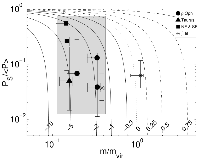
Figure 1: Helical field models are compared with the observed properties of real filaments. Curves are shown for various values of the virial parameter ${\cal M}/|{\cal W}|$. Positive values, corresponding to the dashed curves, indicate that the poloidal field is dominant, while negative values, corresponding to solid curves, indicate that the toroidal field is dominant. The dotted line represents all solutions that are neutrally affected by the helical field (including the unmagnetized solution). The $\int$-shaped filament appears twice, because we have used two independent data sets in our analysis.

Figure 1 demonstrates that most filamentary clouds reside in a part of parameter space where

$$0.11 \stackrel{{\scriptstyle<}}{{\sim}} m/m_{vir}\stackrel{{\scriptstyle<}}{{\sim}}0.43$$

$$0.012 \stackrel{{\scriptstyle<}}{{\sim}} P_{S}/\langle P\rangle\stackrel{{\scriptstyle<}}{{\sim}}0.75,$$

which is indicated by the shaded box in Figure 1. Thus, we find that filamentary clouds range considerably in their virial parameters. However, it is remarkable that most of the clouds in our small data set appear to reside in the part of the diagram where ${\cal M}/|{\cal W}|<0$. Thus, our virial analysis infers that the magnetic field in at least several filamentary clouds is probably helical and toroidally dominated. Gravity and surface pressure alone appear to be insufficient to radially bind the clouds in our sample. While this means that filaments must be quite weakly bound by gravity, we note that similar results have also been obtained by Loren (1989b) and BM92.

It is natural to wonder to what extent these conclusions could be affected by uncertainties in the observational results. The dominant sources of uncertainty in Figure 1 are probably the uncertainties in mass per unit length surface pressures. However, we have assumed very conservative ranges for the surface pressures and inclination angles of the clouds. Therefore, we do not believe that observational uncertainties can account for the helical fields that are required by our virial analysis. We also note that a more detailed model including rotation of the filament would necessarily lead to the same conclusion of a helical field. Since rotation would tend to support the cloud against gravity, even stronger toroidal fields would be required to confine the gas.

3 Exact MHD Models of Filamentary Structure

The virial treatment of the previous section is perhaps the simplest and most illuminating way to understand the physics and global properties of filamentary molecular clouds. While the virial equations 1 and 15 are convenient to use, and are in fact exact expressions of magnetohydrostatic equilibrium, the analysis can say nothing of the internal structure of the clouds. This is the advantage of the exact analytic and numerical models developed in this section.

3.1 The Poloidal and Toroidal Flux to Mass Ratios

We postulate that the magnetic field structure corresponds to that of constant poloidal and toroidal flux to mass ratios $\Gamma_{z}$ and $\Gamma_{\phi}$. The meanings of the flux to mass ratios are illustrated in Figure 2, and are defined in the following way. Consider a bundle of poloidal field lines passing through a small cross-sectional area of the filament $\delta{\cal V}$. The magnetic flux passing through the surface is $B_{z}\delta{\cal V}$, while the mass per unit length is $\rho{\cal V}$. Thus, the ratio of the poloidal flux to the mass per unit length is

$$\Gamma_{z}=\frac{B_{z}}{\rho}.$$ (23)

Is there an analogous quantity for the toroidal component of the field? In fact the toroidal flux has been defined and is commonly used in plasma physics (Bateman 1978). Here, we consider a bundle of toroidal flux lines with cross-sectional area $\delta A$ that form a closed ring of radius $r$ centred on the axis of the filament. The mass enclosed by the ring is $2\pi r\delta A$. Thus, we may define the toroidal flux to mass ratio (per radian) as

$$\Gamma_{\phi}=\frac{B_{\phi}}{r\rho}.$$ (24)

The simplest field configuration is that of constant $\Gamma_{z}$ and $\Gamma_{\phi}$. We note that constant $\Gamma_{\phi}$ results naturally if a filament of constant $\Gamma_{z}$ and length $L$ is twisted uniformly through an angle $\phi$. Then

$$\frac{B_{\phi}}{B_{z}}=\frac{r\phi}{L},$$ (25)

which leads to the result

$$\Gamma_{\phi}=\left(\frac{\phi}{L}\right)\Gamma_{z}.$$ (26)

We shall always assume constant $\Gamma_{z}$ and $\Gamma_{\phi}$ for the remainder of this paper.

Figure 2: A schematic illustration of the poloidal and toroidal flux to mass ratios introduced in equations 23 and 24.

3.2 An Idealized Model: Uniform Magnetized Filaments

As an iside, it is illustrative to consider uniform filamentary clouds are affected by helical fields of constant $\Gamma_{z}$ and $\Gamma_{\phi}$. In this simple model, the magnetic field is uniform within the filament, but drops to zero outside. By equation 24, the toroidal field $B_{\phi}$ increases as $\sim r$ within the filament and falls off as $\sim r^{-1}$ in the external medium. Thus, the toroidal field is associated with a constant poloidal current density within the filament.

With the assumption of constant density and the above definitions of $\Gamma_{z}$ and $\Gamma_{\phi}$, equation 15 can be expanded to give

$$0=\left(\sigma^{2}-\frac{P_{S}}{\rho}+\frac{\Gamma_{z}^{2}\rho}{8\pi}\right)-m\left(\frac{G}{2}+\frac{\Gamma_{\phi}^{2}}{8\pi^{2}}\right).$$ (27)

The critical mass per unit length is obtained by setting $P_{S}=0$:

$$m_{mag}=\frac{2{\sigma^{2}}+\Gamma_{z}^{2}\rho/4\pi}{G+\Gamma_{\phi}^{2}/4\pi^{2}}.$$ (28)

The effects of external pressure and the magnetic field are transparent in this simple model. Pressure and the poloidal field cooperate in supporting the cloud. On the other hand, the toroidal field enters into equation 27 in concert with gravity. A filamentary cloud with a helical field would be confined jointly by gravity, external pressure, and the pinch of the toroidal field. Without prior knowledge of the field strength and direction (by molecular Zeeman and polarization observations), the cloud may appear to be unbound by gravity alone.

3.3 General Equations for Magnetized Filamentary Molecular Clouds

We consider the equilibrium structure of a non-rotating, self-gravitating molecular cloud with a helical field of constant flux to mass ratios $\Gamma_{z}$ and $\Gamma_{\phi}$. We consider two possible equations of state for the gas: 1) the “isothermal” equation of state $P=\sigma^{2}\rho$ where $\sigma$ is the total velocity dispersion and 2) the “pure logatrope” of MP96 given by $P/P_{c}=1+A\ln(\rho/\rho_{c})$, where $P_{c}$ and $\rho_{c}$ are the central (along the filament axis) pressures and densities, and $A$ is a constant. MP96 find $A\simeq 0.2$ for molecular cloud cores. Although their analysis was based only on cloud core data, we shall assume that the same value of $A$ might apply to filamentary clouds as well. We use these two equations of state because they probably bracket the true underlying equation of state for molecular clouds; MHD cloud turbulence probably results in an EOS softer than isothermal (MP96; Gehman et al. 1996), while the pure logatrope is the softest EOS to appear in the literature.

It is convenient to work in dimensionless units where density and pressure are scaled by their central values $\rho_{c}$ and $P_{c}$. We further define the central velocity dispersion by

$$\sigma_{c}^{2}=\frac{P_{c}}{\rho_{c}}.$$ (29)

A natural radial scale is then given by

$$r_{0}^{2}=\frac{\sigma_{c}^{2}}{4\pi G\rho_{c}},$$ (30)

which defines the effective core radius of the filament. Finally, we may define natural scales for the mass per unit length and magnetic field:

$$m_{0} = r_{0}^{2}\rho_{c}=\frac{\sigma_{c}^{2}}{4\pi G}$$

$$B_{0} = P_{c}^{1/2}.$$ (31)

Thus, all quantities are written in dimensionless form as follows:

$${\tilde{r}} = r/r_{0}$$

$${\tilde{\rho}} = \rho/\rho_{c}$$

$${\tilde{m}} = m/m_{0}$$

$${\tilde{P}} = P/P_{c}$$

$${\tilde{\sigma}} = \sigma/\sigma_{c}$$

$${\tilde{\Phi}} = \Phi/\sigma_{c}^{2}$$

$${\tilde{B}_{z}} = B_{z}/B_{0}$$

$${\tilde{B}_{\phi}} = B_{\phi}/B_{0}$$ (32)

Hereafter, we will only ever refer to $\Gamma_{z}$ and $\Gamma_{\phi}$ in their dimensionless forms:

$${\tilde{\Gamma}_{z}} = \sqrt{\frac{\rho_{c}}{\sigma_{c}^{2}}}\left(\frac{B_{z}}{\rho}\right)$$

$${\tilde{\Gamma}_{\phi}} = \frac{1}{\sqrt{4\pi G}}\left(\frac{B_{\phi}}{r\rho}\right)$$ (33)

For brevity, we will drop the tildes for the remainder of this section and the next (except for where ambiguity would result); all quantities hereafter are understood to be written in dimensionless form unless otherwise stated.

Our basic dimensionless equations are those of Poisson

$$\frac{1}{r}\frac{d}{dr}\left(r\frac{d}{dr}\Phi\right)=\rho$$ (34)

and magnetohydrostatic equilibrium

$$\frac{d}{dr}\left(P+\frac{B_{z}^{2}}{8\pi}\right)+\rho\frac{d}{dr}\Phi+\frac{1}{r^{2}}\frac{d}{dr}\left(\frac{r^{2}B_{\phi}^{2}}{8\pi}\right).$$ (35)

In Appendix D, we construct the mathematical framework to solve these equations numerically for both isothermal and logatropic equations of state. We show that a solution to the dimensionless equations is characterized by three parameters, namely the flux to mass ratios $\Gamma_{z}$ and $\Gamma_{\phi}$ defined by equations 23 and 24, and a third to specify the (dimensionless) radius of pressure truncation. We express this third parameter as a concentration parameter defined by $C$ defined as

$$C=\log_{10}\left(\frac{{R_{S}}}{r_{0}}\right),$$ (36)

where $r_{0}$ is the radial scale defined by equation 33. We note that our definition of $C$ is analogous to the concentration parameter $C=\log_{10}(r_{t}/r_{0})$ defined for King models of globular clusters (See Binney & Tremaine 1987). Our concentration parameter differs only in that the tidal radius $r_{t}$ is replaced by the pressure truncation radius, and our $r_{0}$ is smaller by a factor of 3. While we use $C$ primarily as a theoretical parameter, we note that it is in principle observable.

3.4 Analytic Solutions

Before discussing numerical solutions, we derive a few special solutions that can be expressed in closed analytic form. Specifically, we discuss the unmagnetized isothermal solution that was found by Ostriker (1964) (a brief derivation is given in Appendix D.). We note that that this solution is a special case of a more general magnetized solution obtained by Stodólkiewicz (1963); for brevity, we shall refer to this solution as the Ostriker solution for the remainder of this paper. We also find a singular solution for logatropic filaments. It is unlikely that either of these special solutions describe real filaments, which are probably magnetized and non-singular, but they do serve as important benchmark results to compare with our more elaborate magnetized models.

3.4.1 The Ostriker Solution: Unmagnetized Isothermal Filaments

The analytic solution for the special case of an unmagnetized isothermal filament is easily obtained using the mathematical framework in Appendix D. It was first given by Ostriker (1964):

$$\rho=\frac{\rho_{c}}{(1+r^{2}/8r_{0}^{2})^{2}},$$ (37)

where we have restored the dimensional units. We note that the density decreases as $\sim r^{-4}$ at large radii. That such steep density profiles have not been observed could be explained by three possibilities: 1) molecular clouds are not isothermal. A softer EOS would give a less steeply falling density at large radius; 2) real clouds contain dynamically important magnetic fields that modify the structure of the filament at large radius; 3) real filaments are always truncated by external pressure. If the filament is truncated before the $\sim r^{-4}$ envelope is reached, such steep behaviour would not be observed. We demonstrate in Section 4.1.2 that either of possibilities 1) or 2) can explain the observed properties of molecular clouds.

3.4.2 Singular Logatropic Filaments

Although we have been unable to find the analogue of the Ostriker solution for the logatropic EOS, we have been successful in finding a singular solution. For this model, we reinterpret $\rho_{c}$ as the density at some fiducial radius. We postulate a power law solution of the form

$$\rho\propto r^{\alpha},$$ (38)

and find that a solution can only be obtained if $\alpha=-1$. The final solution with dimensional units restored is

$$\frac{\rho}{\rho_{c}}=\sqrt{A}\left(\frac{r}{r_{0}}\right)^{-1}.$$ (39)

It is useful to compare our solution with the singular logatropic sphere found by MP96:

$$\frac{\rho_{sphere}}{\rho_{c}}=\sqrt{2A}\left(\frac{r}{r_{0}}\right)^{-1},$$ (40)

where we have rewritten their solution using our definition of $r_{0}$. (Their definition of $r_{0}$ differs from ours by a factor of 3. Our definition is the customary choice for filaments.). It is remarkable that both singular logatropic spheres and filaments obey precisely the same power law.

4 Numerical Solutions

We now turn our attention to numerical solutions of equation 92 using various values of the flux to mass ratios $\Gamma_{z}$ and $\Gamma_{\phi}$. Many of the solutions are shown out to very large radius but may be truncated to reproduce any desired value of the concentration parameter $C$ defined in equation 36.

4.1 Numerical Results

We have shown in Section 2.4 that many filamentary clouds are probably wrapped by helical magnetic fields. However, before considering the most general case of helical fields in Section 4.1.2, we first separately consider the effects of poloidal and toroidal magnetic fields in Section 4.1.1. We note that purely poloidal fields are not allowed by our virial analysis, and purely toroidal fields are probably unrealistic. Neverthess, this is the best way to understand the roles of each field component in our more general helical field models.

Equation 92 gives the set of differential equations that we integrate to produce our models. The integration was done in a straightforward manner, using a standard Runge-Kutta method.

4.1.1 Models With Purely Poloidal and Toroidal Fields

Figures 3 and 4 show the density and pressure profiles, the magnetic structure, and the mass per unit length for isothermal and logatropic filaments threaded by a purely poloidal field. We have also included the velocity dispersion and average velocity dispersion (given by equation 10) for the logatropic equation of state.

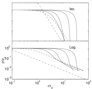
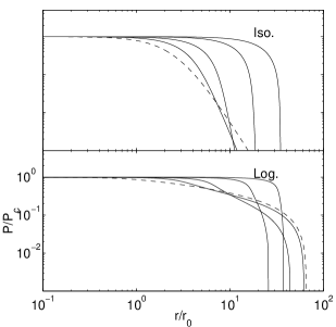
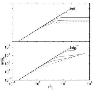
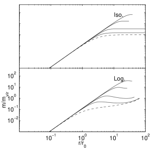
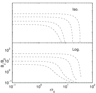
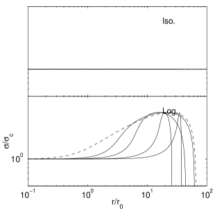
Figure 3: Isothermal and logatropic filaments with purely poloidal magnetic field: $\Gamma_{z}=0$ (dashed line), $5,10,25$ and $50$. The dot-dashed lines represent the $r^{-4}$ density stucture of the Ostriker solution at large radius and the $r^{-1}$ behaviour of the singular logatropic solution.

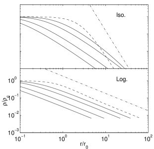
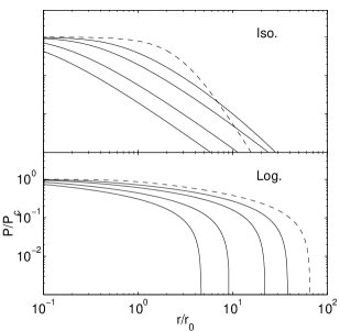
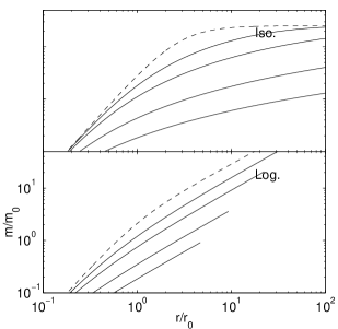
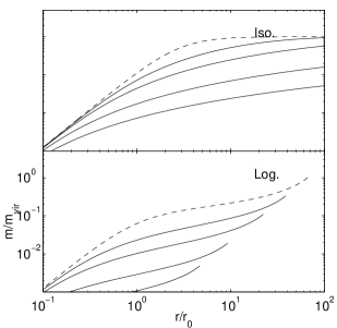
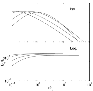
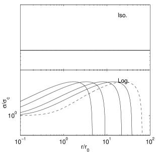
Figure 4: Isothermal and logatropic filaments with purely toroidal magnetic field: $\Gamma_{\phi}=0$ (dashed line), $5,10,25$ and $50$. The dot-dashed lines have the same meaning as in Figure 3.

On each set of figures we have shown the density, pressure, and velocity dispersion structure of the unmagnetized solutions with dashed lines. For isothermal solutions, we have also drawn a line representing the asymptotic $r^{-4}$ behaviour of the Ostriker solution. Similarly, the $r^{-1}$ singular solution has been included on density profiles for logatropic filaments. These power laws are meant as a guide in interpreting the asymptotic behavior of the solutions; we find that they are obeyed at large radius for all unmagnetized filaments.

Comparing the unmagnetized solutions (dashed lines) in Figures 3 and 4, we observe that the density profile of the unmagnetized logatropic filament is slightly more centrally concentrated than the isothermal Ostriker solution, but falls off much less steeply at large radius. These figures also show that isothermal and logatropic filaments both tend to finite mass per unit length, although they differ in that isothermal filaments approach the critical mass per unit length only asymptotically as their radii tend to infinity. As discussed in Section 2, this limit represents the critical mass per unit length $m_{h}$ (see Section 2.1) beyond which no equilibrium is possible. For the isothermal filament, it is easy to show analytically (from equation 37) and we verify numerically that $m_{h}=8\pi m_{0}$, where $m_{0}$ is the mass scale defined by equation 31. For the unmagnetized logatropic filament, we find numerically that $m_{h}=185.8m_{0}$. Logatopic filaments can support a greater mass per unit length for equivalent central velocity dispersion $\sigma_{c}$. This is easily understood since the average velocity dispersion $\langle\sigma^{2}\rangle^{1/2}$ always exceeds the central value offering more turbulent support to the filament.

Perhaps the most notable feature of logatropic filaments is that they “self-truncate” at finite radius and density $\rho=\rho_{c}\exp{(-1/A)}$ where the velocity dispersion and pressure vanish. The logatropic EOS is designed to have a nearly isothermal core and a rising velocity dispersion outside of the core radius. At some point, however, the velocity dispersion turns over and falls to zero. The velocity dispersion could of course never vanish in a real cloud since all real clouds are truncated by finite external pressure. Whether the region of outwardly falling velocity dispersion actually falls within the pressure truncation radius in fits to real clouds is addressed in Section 4.2, where we attempt to constrain our models using the observational results of table 2.

Because of the way in which we have defined $\Gamma_{z}$ (equation 23), $B_{z}$ is exactly proportional to the density. The toroidal field, however, shows a more interesting structure; $B_{\phi}$ always vanishes along the axis of the filament, as it must for the field to be continuous across the axis. We note that the logarithmic radial scale of Figure 4 makes the vanishing of $B_{\phi}$ at the axis difficult to see in some cases. It also is found to decay at large radius for isothermal filaments since $B_{\phi}=\Gamma_{\phi}r\rho\propto r^{-3}$. Hence, there is a single maximum in the toroidal field structure. For logatropic filaments, the $r^{-1}$ asymptotic behaviour of the density implies that $B_{\phi}=\Gamma_{\phi}r\rho$ tends to a constant value at large radius. Thus, the toroidal field in logatropic filaments lacks the local maximum found for isothermal filaments.

The effects of poloidal and toroidal magnetic fields on the density structure are apparent in Figures 3 and 4. For either EOS, the poloidal magnetic field supports the cloud and causes it to be more extended radially than the corresponding unmagnetized filament. Toroidal magnetic fields, on the other hand, pinch the filament to smaller radial extent. Thus, we find our numerical results to be in agreement with the results of our virial analysis in Section 2.

It is significant that purely poloidal fields always steepen the outer density profile, while toroidal fields make it more shallow. For isothermal filaments, poloidal fields always result in density profiles that are steeper than the $r^{-4}$ behaviour of the Ostriker solution; this is true of even logatropic filaments when the field is of sufficient strength. These steep density profiles have never been observed, so purely poloidal fields do not match the data. Thus, it seems likely that the field must have a toroidal component if a realistic density profile is to be achieved.

We find that the magnetic field has a dramatic effect on the critical mass per unit length $m_{mag}$ of the cloud. For either EOS, a poloidal magnetic field increases $m_{mag}$, since the poloidal field acts to support the cloud against self-gravity. The toroidal magnetic field works with gravity, thus decreasing the maximum mass per unit length that can be supported. These conclusions are in agreement with our virial results from Section 2.

From Figures 3 and 4, we note that all isothermal filaments that are unmagnetized or contain a purely toroidal field tend to the same mass per unit length $m_{h}$. This is easily explained by our virial equation 15 since the toroidal field always tends to zero at large radius for isothermal filaments. The critical mass per unit length $m_{mag}$ clearly cannot be affected, since the toroidal field only enters the virial equation through its surface value. This is not the case for logatropic filaments because $B_{\phi}$ tends to a constant value at large radius.

4.1.2 Helical Field Models

In Section 2.4, we provided evidence based on our virial analysis that filamentary clouds likely contain toroidally dominated helical magnetic fields. At this point, we shall take a further step by comparing our exact MHD models with the observed properties of filamentary molecular clouds. As we have noted in Section 4, a numerical solution is completely determined by the choice of three dimensionless parameters; the flux to mass ratios $\Gamma_{z}$, $\Gamma_{\phi}$, and the concentration parameter $C$.

Although ${R_{S}}$ can be observed with little difficulty, obtaining an accurate value for $C$ is difficult because of the uncertainty in the core radius $r_{0}$. According to equation 30, the core radius depends on both the central density and velocity dispersion along the axis of the filament, both of which might be quite uncertain. We can, however, estimate a rough upper bound to $C$ using the data of table 1. We do not presently know whether the central (axial) velocity dispersions of filamentary clouds are dominated by non-thermal motions, as the bulk of the cloud certainly is, or if the velocity dispersions are thermal, as they are in many low-mass cloud cores. Nevertheless, we do know that that $\sigma_{c}$ must be at least the thermal value, which is $0.23~{}km~{}s^{-1}$, assuming a temperature of $15K$. Central densities are probably less than about $10^{4}~{}cm^{-3}$, which is typical of a core. Therefore, equation 30 implies that $r_{0}$ is probably not less than $\approx 0.04~{}pc$. In Table 1, we find that ${R_{S}}\stackrel{{\scriptstyle<}}{{\sim}}0.5~{}pc$ for most (but not all) of the filaments in our sample. Therefore, equation 36 implies that most filamentary clouds should have concentration parameters that are less than approximately 1.1. This estimate should be treated with caution, considering the uncertainties and generalizations in our calculation. In particular, we note that larger filaments, such as the Northern and Southern Filaments in the Orion region (See Table 1) have radii that are many times larger than the value that we used in our calculation and may, therefore, have concentration parameters that exceed our upper bound.

Three observable quantities shall be required to constrain our theoretical models. We have previously (Section 2.4) found the virial parameters $P_{S}/\langle P\rangle$ and $m/m_{vir}$ to be useful in showing that toroidally dominated helical fields play an important role in the virial equilibrium of filamentary clouds. We use these parameters, as well as a third parameter specifying the ratio of average magnetic to kinetic energy densities to constrain our models. Accordingly, we define a virial parameter

$$X=\frac{M}{K},$$ (41)

where $M$ and $K$ are the average magnetic and kinetic energy densities within the cloud defined by

$$M = \frac{\int_{V}(B_{z}^{2}+B_{\phi}^{2})dV}{8\pi V}$$

$$K = \frac{3}{2}\langle\rho\rangle\langle\sigma^{2}\rangle,$$ (42)

and $V$ is the volume of the cloud (not to be confused with ${\cal V}$). Myers and Goodman (1988a,b) have provided considerable observational evidence that the average magnetic and kinetic energy densities are in approximate equipartition, with $M\approx K$ to within a factor of order 2. Therefore, we impose the auxiliary constraint that

$$X\approx{\cal O}[1]$$ (43)

for filamentary clouds with realistic magnetic fields. This equipartition of energy has been explained by attributing the non-thermal motions within molecular clouds to internally generated Alfvénic turbulence (BM92). Since super-Alfvénic turbulence is highly dissipative, the Alfvén speed poses a natural limit for the non-thermal velocity dispersion (BM92). Thus, we expect $\sigma\approx v_{A}$ for molecular clouds. Defining the average squared Alfvén speed as

$$\langle v_{A}^{2}\rangle=\frac{\int_{0}^{m}v_{A}^{2}dm^{\prime}}{m},$$ (44)

it is easy to show that

$$X=\frac{\langle v_{A}^{2}\rangle}{3\langle\sigma^{2}\rangle}.$$ (45)

Therefore, $X\approx 1$ is a natural result for magnetized clouds supported against gravity by Alfvénic turbulence. In the analysis that follows, we assume that

$$0.2\leq X\leq 5$$ (46)

for all reasonable models and that $0.5\leq X\leq 2$ is appropriate for our most realistic models.

4.1.3 Monte Carlo Exploration of the Parameter Space

In this Section, we perform a Monte Carlo sampling of our parameter space in order to determine which values of $\Gamma_{z}$, $\Gamma_{\phi}$, and $C$ result in models that obey all of our constraints. The Monte Carlo analysis is very straightforward. We simply assign random values to the three theoretical parameters and compute helical field models using the mathematical framework of Section 3.3. Once a solution has been obtained, we compute $m/m_{vir}$, $P_{S}/\langle P\rangle$, and $X$ using equations 12, 9, and 41, from which we easily determine whether or not the solution obeys our constraints. Figure 5 shows the results of our Monte Carlo analysis for isothermal models, while Figure 6 shows the results for logatropic models. Each point in these figures represents a model that obeys our constraints on $m/m_{vir}$ and $P_{S}/\langle P\rangle$; models that fall outside of these constraints have been discarded.

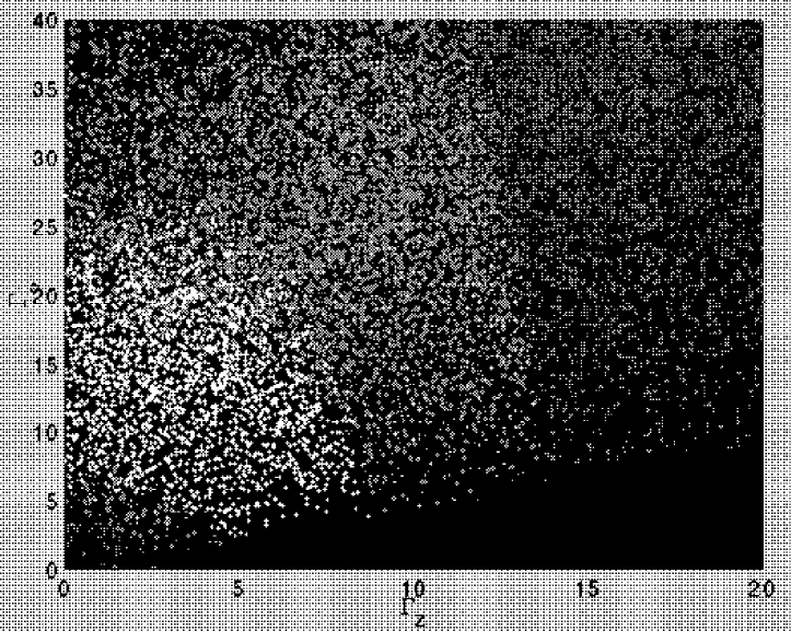
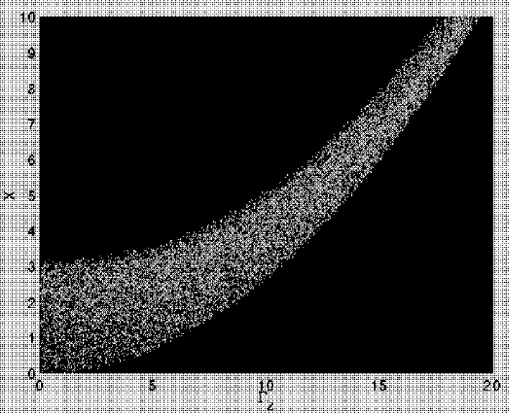
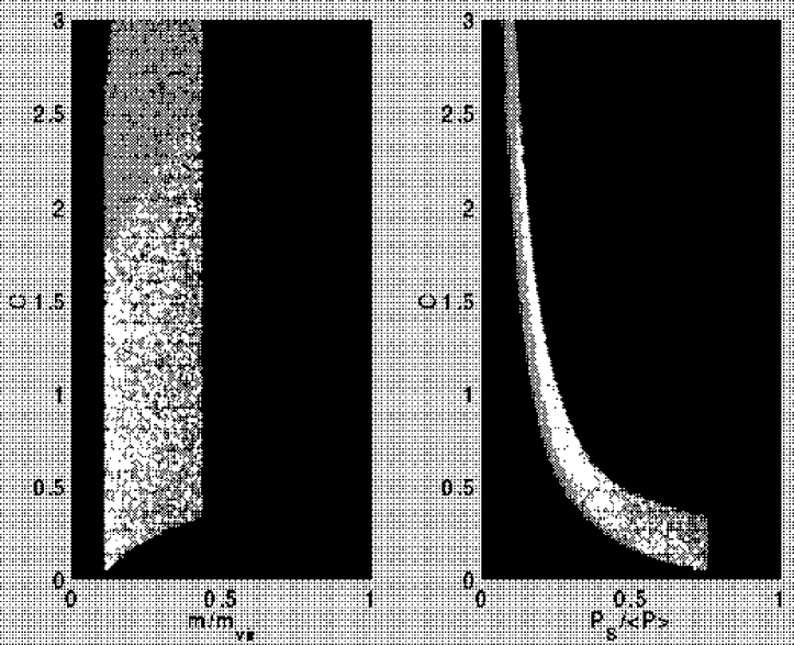
Figure 5: Isothermal Models. We show the results of our Monte Carlo exploration for isothermal filaments. Each point on these figures represents a model that obeys the observational constraints given in equation LABEL:eq:constraints; thus, we determine which ranges of $\Gamma_{z}$, $\Gamma_{\phi}$, and $C$ result in models that agree with the available observational data. a) (top) The grayscale represents different ranges for $X$, as defined in equation 41. The most realistic solutions, with $0.5\stackrel{{\scriptstyle<}}{{\sim}}X\stackrel{{\scriptstyle<}}{{\sim}}2$ are shown as white dots. The medium gray dots have $0.2\stackrel{{\scriptstyle<}}{{\sim}}X\stackrel{{\scriptstyle<}}{{\sim}}5$. The dark gray dots represent models that are outside of these ranges with unrealistic magnetic field strengths. b) (middle) We show that $X$ is determined mainly by $\Gamma_{z}$. c) (bottom) We show the allowed ranges of the concentration parameter $C$. The shading is the same as in a). However, we note that the darkest gray dots are mostly hidden “behind” the medium gray, in this case.

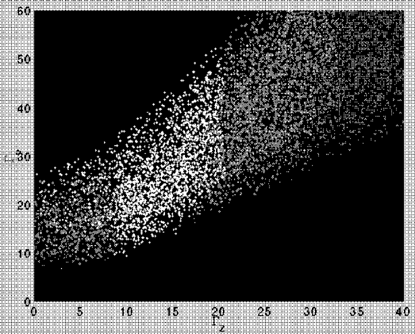
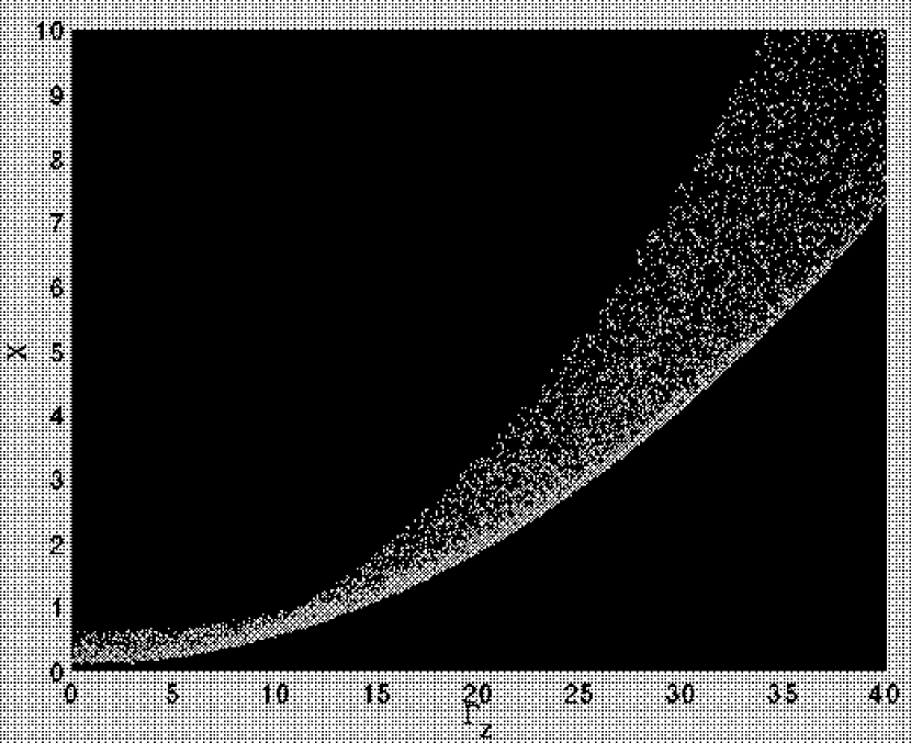
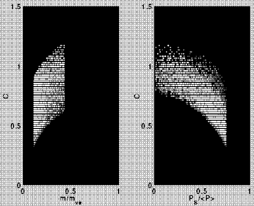
Figure 6: Logatropic Models. We show the results of our Monte Carlo analysis for logatropic filaments. The graphs are as described in the caption of Figure 5.

The grayscale in Figures 5a and 6a represent different ranges for $X$. The most likely range of $X$, with $0.5\leq X\leq 2$ is shown as the lightest coloured points. The next darkest gray dots represent a less likely, but still possibly allowed range, with $0.2\leq X\leq 5$, while the darkest gray dots represent models that are outside of these ranges, and therefore have unrealistically large or small magnetic fields. It should be noted that there relatively little overlap between these regions; they map out quite distinct regions on the diagrams. From Figure 5a, we find that the allowed ranges for the flux to mass ratios are approximately

$$5~{}\stackrel{{\scriptstyle<}}{{\sim}}~{}\Gamma_{\phi} \stackrel{{\scriptstyle<}}{{\sim}} 25$$

$$\Gamma_{z} \stackrel{{\scriptstyle<}}{{\sim}} 8$$ (47)

for isothermal filaments with $0.5\leq X\leq 2$. A somewhat larger region of the parameter space is allowed for filaments with $0.2\leq X\leq 5$. Comparing with Figure 6a, we find that the allowed flux to mass ratios are somewhat larger for logatropic filaments, where we find

$$10~{}\stackrel{{\scriptstyle<}}{{\sim}}~{}\Gamma_{\phi} \stackrel{{\scriptstyle<}}{{\sim}} 40$$

$$10~{}\stackrel{{\scriptstyle<}}{{\sim}}~{}\Gamma_{z} \stackrel{{\scriptstyle<}}{{\sim}} 20$$ (48)

when $0.5\leq X\leq 2$. We note that $\Gamma_{z}$ is more tightly constrained than $\Gamma_{\phi}$ for both isothermal and logatropic filaments.

In Figures 5b and 6b, we plot the our magnetic parameter $X$, for the allowed models, against the poloidal flux to mass ratio $\Gamma_{z}$. We find that $X$ has a very strong dependance on $\Gamma_{z}$ for both isothermal and logatropic models. Moreover, we find that there is no obvious correlation between $X$ and $\Gamma_{\phi}$. Since we can regard $X$ as nearly a function of $\Gamma_{z}$ alone, the auxiliary constraint on $X$ directly constrains $\Gamma_{z}$. It is for this reason that somewhat tighter contraints are obtained on $\Gamma_{z}$ in equations 47 and 48, than on $\Gamma_{\phi}$.

Figures 5c and 6c show the dependence of the concentration parameter $C$ on $m/m_{vir}$ and $P_{S}/\langle P\rangle$ for models that are allowed by the observations. We find that $C$ may range from 0 to $\approx 3$ for isothermal models, but $C\stackrel{{\scriptstyle<}}{{\sim}}1.7$ for most solutions where $0.5\leq X\leq 2$. Moreover, we find that $C$ correlates rather well with $P_{S}/\langle P\rangle$, with greater values of $P_{S}/\langle P\rangle$ corresponding to smaller values of $C$. We note that most filamentary clouds probably have $C\stackrel{{\scriptstyle<}}{{\sim}}1.1$, considering our discussion in Section 4.1.2. However, we do not enforce this upper bound as a rigid constraint, since further data on the central densities and velocity dispersions of filamentary clouds needs to be obtained in order to make our argument definitive. We find that $C\stackrel{{\scriptstyle>}}{{\sim}}1$ whenever $P_{S}/\langle P\rangle\stackrel{{\scriptstyle<}}{{\sim}}0.25$; therefore, isothermal filaments with $C\stackrel{{\scriptstyle<}}{{\sim}}1$ must be subject to external pressures that are at least one fourth of the mean internal pressure. Such relatively high external pressures are well within the range of pressures allowed by equation LABEL:eq:constraints. The concentration parameter $C$ is much more restricted for logatropic models, where $C$ may range only from aprroximately 0.4 to 1.2. As a general trend, we find that $C$ increases slightly with $m/m_{vir}$, and also as $P_{S}/\langle P\rangle$ decreases. This is a natural result, since filaments become more radially extended, with greater $C$, as they become closer to their critical configurations with vanishing $P_{S}/\langle P\rangle$ and maximum $m/m_{vir}$.

4.2 “Best-Fitting” Models For Magnetized Filamentary Clouds

In Figure 7, we show 50 isothermal helical field models that span the range of parameters allowed by equations LABEL:eq:constraints and 46. We see that our allowed models possess a number of very robust characteristics. Most importantly, we find that most of our isothermal models have outer density profiles that fall off as $\sim r^{-1.8}$ to $r^{-2}$, with some of most truncated models having somewhat more shallow profiles. This is most clearly shown in Figure 7b, where we have plotted the power law index $\alpha=d\ln{\rho}/d\ln{r}$ as a function of the dimensionless radius $r/r_{0}$. We observe that $\alpha$ becomes more negative with increasing radius, but that none of our models ever have density profiles that are steeper than $r^{-2}$. Thus, we find that our isothermal helical field models have density distributions that are much more shallow than the $r^{-4}$ Ostriker solution. This radical departure from the Ostriker solution is clearly due to the dominance of the magnetic field over gravity in the outer regions. The overall effect of the helical field is to modify the density structure of the Ostriker solution so that a much more realistic form is obtained. In particular, we note that A98 and LAL98 have recently used extinction measurements of background starlight in the near infra-red to show that two filamentary clouds, namely L977 and IC 5146, have $r^{-2}$ density distributions. Our helical field models have density profiles that are essentially the same as those obtained for models with purely toroidal fields in Section 4.1.1. Therefore, we conclude that the outer density distribution is shaped primarily by the toroidal component of the field. We note, however, that the toroidal field is in fact much weaker than the poloidal field throughout most of a filamentary cloud. In all cases, the basic magnetic structure is that of a poloidally dominated core region surrounded by a toroidally dominated envelope, where the field is relatively weak.

In Figure 8, we show a sample of 50 logatropic models that are allowed by our constraints. The main difference between the logatropic models and the isothermal models shown in Figure 7 is that there is a much greater variety of allowed density distributions for the logatropes. We find logatropic filaments with density profiles as shallow as $r^{-1}$ and as steep as $r^{-1.8}$. Unlike the isothermal solutions, $\alpha$ does not decrease monatonically. Rather, it usually reaches a minimum value somewhat less than -1 when $r/r_{0}\approx 1$ to $3$, and increases at larger radii. The result is that the density distribution usually contains a small region where the density falls quite rapidly, which is surrounded by an envelope with a more gentle power law. Many logatropic models have density profiles that are too shallow to explain the A98 and LAL98 data. However, we have also found many logatropic models that approach the observed $r^{-2}$ profiles. The main difference between isothermal and logatropic models is that isothermal filaments produce a nearly “universal” $r^{-1.8}$ to $r^{-2}$ density profile, while logatropic filaments show a much larger range of behaviour.

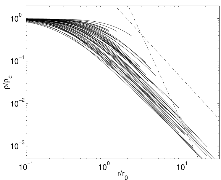
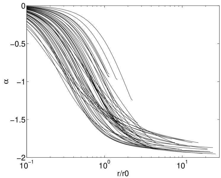
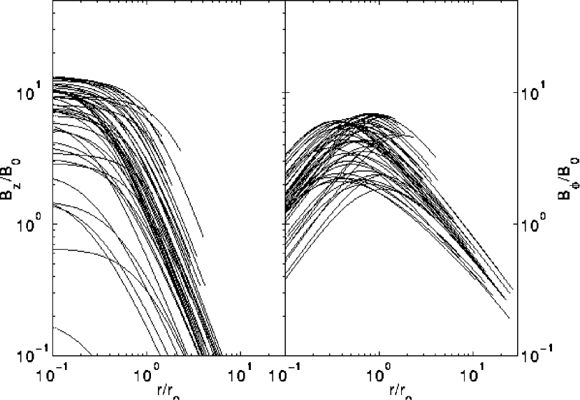
Figure 7: We show a sample of 50 isothermal models that span the range of allowed parameters given in equations LABEL:eq:constraints and 46. a) (top) We show the density profiles of the models. The dashed lines represent the $r^{-4}$ density profile of the Ostriker solution and an $r^{-2}$ profile, which is in agreement with the observed density profiles of filamentary clouds (Alves et al. (1998), Lada, Alves, and Lada (1998)). b) (middle) We show the how the power law index $d\ln{\rho}/d\ln{r}$ behaves with radius. c) (bottom) We show the behaviour of the poloidal and toroidal components of the magnetic field.

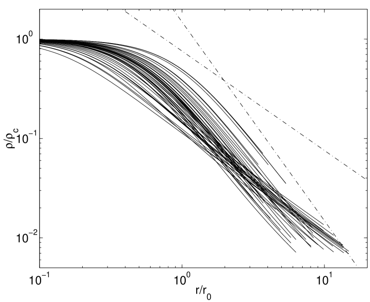
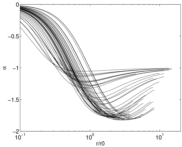
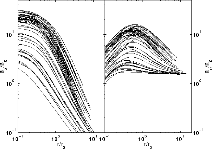
Figure 8: We show a sample of 50 logatropic models that span the range of allowed parameters given in equations LABEL:eq:constraints and 46. a) (top) We show the density profiles of the models. The dashed lines represent the $r^{-4}$ density profile of the Ostriker solution and an $r^{-2}$ profile, which is in agreement with the observed density profiles of filamentary clouds (Alves et al. (1998), Lada, Alves, and Lada (1998)). b) (middle) We show the how the power law index $d\ln{\rho}/d\ln{r}$ behaves with radius. c) (bottom) We show the behaviour of the poloidal and toroidal components of the magnetic field.

5 Discussion

We show, in Section 2.4, that most of the filamentary molecular clouds in our sample have velocity dispersions that are too high for them to be bound by gravity and surface pressure alone. Thus, we find evidence that many filamentary clouds are probably wrapped by helical magnetic fields whose toroidal components help to confine the gas by the hoop stress of the curved field lines. It is important to realize that this conclusion is based on our virial analysis of filamentary clouds (Section 2) and is, therefore, independent of either the EOS of the gas or the mass loading of the magnetic field lines. We find that all of the filamentary clouds in our sample have masses per unit length that are much lower than the critical mass per unit length for purely hydrostatic filaments, and that filaments are quite far from their critical configurations, where $P_{S}/\langle P\rangle\rightarrow 0$ (See equation LABEL:eq:constraints.). Thus, star formation in filamentary clouds must involve fragmentation into periodic cores (cf. Chandrasekhar & Fermi 1953), rather than overall radial collapse. We refer to the second paper in our series for a full analysis of this process.

We construct numerical MHD models of filamentary clouds, which we explore thoroughly in Section 4.1.3 using Monte Carlo techniques. We show that both isothermal and logtropic models are consistent with the available observational data. We find that helical fields have profound effects on the outer density profiles of filamentary clouds. While hydrostatic filaments have a density profile that falls off as $r^{-4}$ (see Section 3.4.1), nearly all of our isothermal models with helical fields have much more shallow density profiles that fall off as $r^{-1.8}$ to $r^{-2}$. The toroidal component of the field is entirely responsible for these shalow density profiles. Logatropic models show a a greater variety of behaviour, with density profiles ranging from $r^{-1}$ to $r^{-1.8}$. We note nearly all of our isothermal models and many of our logatropic models are in excellent agreement with the $r^{-2}$ density profiles of the filamentary clouds L977 and IC 5146, which have recently been observed by A98 and LAL98. Helical fields, rather than the nature of the EOS, seem to explain the data by controlling the density profiles.

The confirmation of helical fields in filamentary clouds will ultimately require direct observations of the field structure using sub-mm polarization and possibly molecular Zeeman observations. Unfortunately, most polarization observations of molecular clouds have been carried out in the optical and near infra-red regions of the spectrum; Goodman et al. (1995) have demonstrated that such measurements are likely a poor indicator of magnetic field direction in cold dark clouds. More promising is the prospect of observing the thermal dust grain emission of dark clouds, which will hopefully become commonplace in the near future with instruments like the SCUBA polarimeter. In emission, we can be assured that any polarization is due to warm dust grains within the cloud being observed. The observational verification of our helical field models for filamentary molecular clouds will need to rely heavily on such observations.

5.1 Observational Signatures of Helical Magnetic Fields

Helical magnetic fields present an interesting and unique polarization pattern. One might expect to find polarization vectors aligned with some average pitch angle of the magnetic field. However, Carlqvist (1997) has modeled the polarization pattern of helical magnetic fields and demonstrated that this assumption is incorrect. The signature of a helical field, assuming that the polarization percent remains small and that the cloud is optically thin, is actually polarization vectors that are either aligned with or perpendicular to the filament axis with a possible $90^{o}$ change in orientation at some radius. The reason for this counterintuitive behaviour is that any line of sight through the filament intersects a given radius not once, but twice. Since the order of polarizing elements is unimportant in the limit of small polarization, the combination of any symmetric pair of polarizing elements results in a cancelation of any oblique component of the net polarization. Although Carlqvist’s model was done for absorption polarimetry, the same reasoning holds for emission. The overall pattern will only reflect the dominant component of the field along any line of sight; thus, our models predict that the innermost (poloidally dominated) regions of filamentary clouds should be dominated in emission by polarization vectors aligned perpendicular to the filament, while the polarization should be predominantly parallel to the filament in the (toroidally dominated) outer regions.

There is some direct evidence that filamentary clouds contain helical magnetic fields. Optical polarization and HI Zeeman data are consistent with a helical field in the large Orion A filament oriented at an approximately $20^{o}$ pitch angle relative to the axis of the filament (Bally 1989). While the reliability of the optical polarization data is uncertain due to the reasons discussed above, the Zeeman observations do not suffer such ambiguity. The line of sight component of the magnetic field has been observed to reverse across the L1641 portion of the filament (Heiles 1987, 1989). Such a reversal is very suggestive of a helical field wrapped around the cloud. More recently, Heiles (1997) has suggested that an alternate explanation might be that the shock front of the Eridanus superbubble has swept past the Orion A cloud causing field lines to be stretched over the filament, thus simulating a helical pattern. While Heiles favours this idea, he cannot rule out the the older idea that the field is intrinsically helical. Regardless of the true nature of the $\int$-shaped filament, we observe that it is one of the few filaments shown in Figure 1 where our models do not actually require a helical field for equilibrium.

6 Summary

1. All filamentary molecular clouds are truncated by external pressure that provides a total (thermal plus turbulent) pressure which is likely in the range of $10^{4}$ to $10^{5}~{}Kcm^{-3}$.

2. We have derived a new form of the virial theorem appropriate for filamentary molecular clouds that are truncated by a realistic external pressure and contain ordered magnetic fields. We have collected data on filamentary clouds from the literature. We find that most of the filamentary clouds in our sample are constrained by

$$0.11 \stackrel{{\scriptstyle<}}{{\sim}} m/m_{vir}\stackrel{{\scriptstyle<}}{{\sim}}0.43$$

$$0.012 \stackrel{{\scriptstyle<}}{{\sim}} P_{S}/\langle P\rangle\stackrel{{\scriptstyle<}}{{\sim}}0.75.$$

We use these observational constraints to show that many filamentary clouds are likely wrapped by helical magnetic fields.

3. We have used our virial equation to derive virial relations for filaments that are analogous to the well-known relations for spheroidal equilibria (Chièze 1987; Elmegreen 1989; MP96). We find that the virial relations for filaments differ from the corresponding relations for spheroids only by factors of order unity.

4. We have studied the stability of filamentary molecular clouds in the sense of Bonnor and Ebert. We find that all filamentary molecular clouds, that are initially in equilibrium, are stable against radial perturbations. Thus, a cloud that is initially in equilibrium cannot be made to undergo radial collapse by increasing the external pressure; the only way to destabilize a filament against radial collapse is by increasing its mass per unit length beyond a critical value that depends on the magnetic field. This critical value is the maximum mass per unit length for which any equilibrium is possible; for purely hydrostatic filaments, the critical mass per unit length is given by $m_{h}=2\langle\sigma^{2}\rangle/G$ (See Section 2.1). The poloidal component of the magnetic field increases the critical mass per unit length by supporting the gas against self-gravity. The toroidal field works with gravity in compressing the filament; thus, the toroidal field decreases the critical mass per unit length.

5. There are two exact analytic solutions that can be found in the limit of vanishing magnetic field. Stodólkiewicz (1963) and Ostriker (1964) have found the equilibrium solution for unmagnetized isothermal filaments; the density in this solution tends to an $\sim r^{-4}$ behaviour outside of the core radius. A98 and LAL98 have shown that the filamentary clouds L977 and IC 5146 have density profiles that fall off as $r^{-2}$. If this result holds true for other filaments as well, it is unlikely that the Ostriker solution describes real molecular filaments. In addition, we have found a singular solution for unmagnetized logatropic filaments. The density profile of this filament is much more shallow; it falls off only as $r^{-1}$, which is probably too shallow to agree with observational results.

6. We have constructed exact numerical MHD models for filamentary clouds in Sections 4 and 4.1. We have considered both isothermal and logatropic equations of state, which likely bracket the true underlying EOS for filamentary molecular clouds. The magnetic field structure is more general than in previous studies; we have assumed only that the poloidal and toroidal flux to mass ratios ($\Gamma_{z}$ and $\Gamma_{\phi}$) are constant, which we justify in Section 3.2.

7. Isothermal models with purely poloidal magnetic fields have density profiles that are even steeper than the Ostriker solution; it is unlikely that such models describe real molecular clouds. Toroidal fields result in density profiles that are more shallow than the Ostriker solution (typically $r^{-2}$ profiles), and in better agreement with observations.

8. We have performed a Monte Carlo analysis of our models, in which we randomly sample our parameter space and then determine whether or not the resulting model agrees with the observational constraints (equations LABEL:eq:constraints and 46). We find both isothermal and logatropic filaments that are allowed by the data. We find that

$$5~{}\stackrel{{\scriptstyle<}}{{\sim}}~{}\Gamma_{\phi} \stackrel{{\scriptstyle<}}{{\sim}} 25$$

$$\Gamma_{z} \stackrel{{\scriptstyle<}}{{\sim}} 8$$ (50)

for isothermal filaments, and

$$10~{}\stackrel{{\scriptstyle<}}{{\sim}}~{}\Gamma_{\phi} \stackrel{{\scriptstyle<}}{{\sim}} 40$$

$$10~{}\stackrel{{\scriptstyle<}}{{\sim}}~{}\Gamma_{z} \stackrel{{\scriptstyle<}}{{\sim}} 20$$ (51)

for logatropic filaments.

9. Our best-fitting isothermal models have density profiles that fall off as only $\sim r^{-1.8}$ to $\sim r^{-2}$, in contrast to the $r^{-4}$ behaviour of the Ostriker solution. These shallow profiles are entirely due to the effects of the toroidal component of the magnetic field. Thus, helical magnetic fields are necessary for reasonable models of isothermal filaments. The logatropic filaments show a greater variet of density profiles that range from $r^{-1}$ to $r^{-1.8}$. Thus, some of the logatropic filaments may agree with the observed $r^{-2}$ profiles (A98 and LAL98), while others may be somewhat too shallow.

7 Acknowledgements

The authors wish to acknowledge Christopher McKee and Dean McLaughlin for their many insightful comments. J.D.F. acknowledges the financial support of McMaster University and an Ontario Graduate Scholarship. The research grant of R.E.P. is supported by a grant from the Natural Sciences and Engineering Research Council of Canada.

Appendix A Derivation of the Virial Equation for Filamentary Molecular Clouds

The tensor virial theorem is written in its most general form as

$$\frac{1}{2}\frac{d^{2}I_{ik}}{dt^{2}} = 2T_{ik}+\delta_{ik}\left[\int_{V}PdV+M_{V}\right]+W_{ik}-2M_{ik}$$ (52)

$$+ \int_{S}x_{k}\left(\frac{B_{i}B_{j}}{4\pi}dS_{j}-\frac{B^{2}}{8\pi}dS_{i}\right)-\int_{s}Px_{k}dS_{i},$$

(Chandrasekhar 1961) where we work in Cartesian coordinates $x_{i}$, and the integration is over the volume $V$ of the cloud bounded by surface $S$. Here, $P$ is the total pressure (with both thermal and non-thermal contributions) and $I_{ik}$, $T_{ik}$, $W_{ik}$, and $M_{ik}$ are respectively the Cartesian tensors for moment of inertia, kinetic energy, gravitational potential, and magnetic energy. The pressure and magnetic field both contribute bulk terms that support the cloud and surface terms that confine the gas. The magnetic term $M_{V}$ is just the bulk component of the magnetic energy:

$$M_{V}=\frac{1}{8\pi}\int B^{2}dV$$ (53)

where $B$ is the magnitude of the magnetic field. The tensor components are given by

$$I_{ik} = \int dV\rho x_{i}x_{k}$$

$$T_{ik} = \frac{1}{2}\int dV\rho v_{i}v_{k}$$

$$W_{ik} = -\int dV\rho x_{k}\frac{\partial\Phi}{\partial x_{i}}$$

$$M_{ik} = \frac{1}{8\pi}\int dVB_{i}B_{k},$$ (54)

where $\rho$ is density, $P$ is pressure, $v_{i}$ and $B_{i}$ are components of velocity and magnetic field, and $\Phi$ is the gravitational potential.

A filamentary molecular cloud may be idealized as a cylinder whose length greatly exceeds it radius. The most appropriate scalar virial equation for such an object is obtained by taking the sum of the $x$ and $y$ (11 and 22) diagonal components of the tensor virial equation 52; the $z$ component can be ignored because we are concerned only with equilibrium in the radial direction. Considering the surface $S$ to be the boundary of a filament of total volume $V$, we expand the $i$th diagonal component of equation 52 using the definitions 54:

$$\frac{1}{2}\frac{d^{2}I_{ii}}{dt^{2}} = \int_{V}PdV-\int_{S}Px_{i}dS_{i}-\int_{V}\rho x_{i}\frac{\partial\Phi}{\partial x_{i}}dV$$ (55)

$$+ \frac{1}{8\pi}\int_{V}B^{2}dV-\frac{1}{4\pi}\int_{V}B_{i}^{2}dV$$

$$+ \frac{1}{4\pi}\int_{S}(x_{i}B_{i})(B_{j}dS_{j})-\frac{1}{8\pi}\int_{S}B^{2}x_{i}dS_{i},$$

where summation over index $j$ is implied, but no sum is to be taken over index $i$. We have also used the fact that the kinetic energy tensor $T_{ik}$ vanishes, since the velocity is everywhere zero. Summing over components $11$ and $22$ and setting $\ddot{I}_{11}=\ddot{I}_{22}=0$ for a filamentary cloud in equilibrium, we easily obtain

$$0 = 2\int_{V}PdV-\int_{S}P{\bf r}\cdot d{\bf S}-\int_{V}\rho{\bf r}\cdot{\bf\nabla}\Phi dV$$ (56)

$$+ \frac{1}{4\pi}\int_{V}B^{2}dV-\frac{1}{4\pi}\int_{V}(B_{x}^{2}+B_{y}^{2})dV$$

$$+ \frac{1}{4\pi}\int_{S}({\bf r}\cdot{\bf B})({\bf B}\cdot d{\bf S})-\frac{1}{8\pi}\int_{S}B^{2}{\bf r}\cdot d{\bf S},$$

where the position vector ${\bf r}$ and surface element $d{\bf S}$ are defined by

$${\bf r} = x\hat{x}+y\hat{y}$$

$$d{\bf S} = dS_{x}\hat{x}+dS_{y}\hat{y}.$$ (57)

Assuming that the magnetic field is helical, it is obvious that ${\bf B}\cdot d{\bf S}=0$; thus, the first magnetic surface term on line 3 of equation 68 is identically zero. Simplifying equation 56 and dividing by the length, we obtain the form of the virial equation most appropriate for filamentary equilibria:

$$0 = 2\int Pd{\cal V}-2P_{S}{\cal V}-\int_{\cal V}\rho r\frac{\partial\Phi}{\partial r}d{\cal V}$$ (58)

$$+ \frac{1}{4\pi}\int B_{z}^{2}d{\cal V}-\left(\frac{B_{zS}^{2}+B_{\phi S}^{2}}{4\pi}\right){\cal V}.$$

It is interesting to note that this may be rewritten as

$$0=\frac{4}{3}{\cal U}\left(1-\frac{P_{S}}{\langle P\rangle}\right)+{\cal W}+{\cal M},$$ (59)

where ${\cal U}$ is the internal energy per unit length:

$${\cal U}=\frac{3}{2}\int_{\cal V}\rho{\sigma^{2}}d{\cal V}.$$ (60)

Thus, we see that our virial equation for filamentary equilibria does in fact differ substantially from the usual form for spheroids.

Appendix B Bonnor-Ebert Stability of Magnetized Filaments

We have shown, in Section 2, that all hydrodynamic filaments, which are initially in equilibrium, are stable in the sense of Bonnor (1956) and Ebert (1955). In this section, we examine the Bonnor-Ebert stability of uniform magnetized filaments.

B.1 Uniform Clouds

We begin by considering a radial perturbation of a uniform filament in which the mass per unit length and the velocity dispersion are conserved. Solving equation 27 for the external pressure, we easily obtain

$$P_{S}=\frac{c_{\phi}}{{\cal V}}+\frac{c_{z}}{{\cal V}^{2}},$$ (61)

where

$$c_{\phi} = m{\sigma^{2}}-m^{2}\left(\frac{G}{2}+\frac{\Gamma_{\phi}^{2}}{8\pi}\right)$$

$$c_{z} = \frac{m^{2}\Gamma_{z}^{2}}{8\pi}.$$ (62)

Differentiating with respect to ${\cal V}$ and simplifying using equations 61, 62, 23, and 9, we obtain

$$\frac{dP_{S}}{d{\cal V}}=-\frac{1}{{\cal V}}\left(P_{S}+P_{mag}\right)<0$$ (63)

for all choices of ${\cal V}$ and $P_{S}$. We conclude that all uniform filaments in equilibrium (having $m<=m_{mag}$) are stable in the sense of Bonnor and Ebert.

B.2 Non-Uniform Clouds

We now extend the argument to general magnetized filamentary equilibria using the mathematical framework of Section 3.3 and Appendix D.

Again we consider a radial perturbartion of a filamentary cloud in which the mass per unit length $m$ is conserved. Following MP96, we shall also require that the central velocity dispersion $\sigma_{c}$ remain unchanged. Referring to equations 31 and 33, we may write

$${\tilde{m}}=\frac{m}{m_{0}}=\frac{4\pi Gm}{\sigma_{c}^{2}}.$$ (64)

Thus, we see that the dimensionless mass per unit length ${\tilde{m}}$ is also conserved during the perturbation. Since ${\tilde{m}}$ is implicitly a function of ${\tilde{r}}$ alone, the dimensionless radius ${\tilde{R_{S}}}$ must remain fixed during the perturbation. Therefore, we find that the radial perturbation takes the form of a simple rescaling of the dimensionless solution with none of the dimensionless variables perturbed whatsoever. With this result in hand, we write

$$P_{S} = P_{c}{\tilde{P}_{S}}=\sigma_{c}^{2}\rho_{c}{\tilde{P}_{S}}$$

$${R_{S}} = \sqrt{\frac{\sigma_{c}^{2}}{4\pi G}}\rho_{c}^{-1/2}{\tilde{R_{S}}},$$ (65)

where $\sigma_{c}$, ${\tilde{P}_{S}}$, and ${\tilde{R_{S}}}$ all remain fixed during the perturbation. Eliminating $\rho_{c}$, we obtain the result

$${R_{S}}=\sqrt{\frac{\sigma_{c}^{4}}{4\pi G}}({\tilde{P}_{S}}{\tilde{R_{S}}}^{2})^{1/2}P_{S}^{-1/2}.$$ (66)

Since ${R_{S}}\propto P_{S}^{-1/2}$, we find that

$$\frac{d{R_{S}}}{dP_{S}}<0$$ (67)

for all external pressures $P_{S}$. Therefore, we conclude that all self-gravitating filaments that are initially in a state of equilibrium (which requires $m\leq m_{mag}$ by equation 18), are stable in the sense of Bonner and Ebert.

Appendix C Virial Relations and Larson’s Laws for Filaments

We derive the virial relations for filamentary molecular clouds analogous to the well known relations for spheroidal clouds (Chièze 1987; Elmegreen 1989; MP96). Using equation 7 in our virial equation for filamentary clouds (equation 1), we write

$$0=2m\langle\sigma^{2}\rangle-2P_{S}{\cal V}-am^{2}G+{\cal M}$$ (68)

We have shown in Section 2 that the constant $a$ is exactly unity for any filament but we retain the constant in order to more directly compare with the corresponding expressions for spheroidal clouds. Equation 68 can be rewritten as

$$\alpha_{mag}=a\frac{1-{\cal M}/|{\cal W}|}{1-P_{S}/\langle P\rangle}\equiv\frac{m_{vir}}{m}$$ (69)

where we have introduced the observable virial parameter $\alpha_{mag}$ for filamentary clouds analogous to that of Bertoldi and McKee (1992, hereafter BM92). We may also write

$$\alpha_{mag}=\alpha_{non}\left(1-\frac{{\cal M}}{|{\cal W}|}\right),$$ (70)

where $\alpha_{non}$ is just $\alpha_{mag}$ evaluated in the unmagnetized limit:

$$\alpha_{non}=\frac{a}{1-P_{S}/\langle P\rangle}.$$ (71)

Equations 69 and 71 are easily solved for the mass per unit length $m$, radius ${R_{S}}$, average density $\langle\rho\rangle$, and surface density $\Sigma$. In order to compare with the corresponding results for spheroidal magnetized equilibria (See MP96), we present the results as general expressions with the coefficients written in table 3:

$$m = C_{m}\frac{\langle\sigma^{2}\rangle}{\alpha_{mag}G}$$

$$R = C_{R}\left(\frac{\alpha_{non}-a}{\alpha_{non}}\right)^{1/2}\frac{1}{\alpha_{mag}^{1/2}}\frac{\langle\sigma^{2}\rangle}{(GP_{S})^{1/2}}$$

$$\langle\rho\rangle = C_{\rho}\left(\frac{\alpha_{non}}{\alpha_{non}-a}\right)\frac{P_{S}}{\langle\sigma^{2}\rangle}$$

$$\Sigma = C_{\Sigma}\frac{1}{\alpha_{mag}^{1/2}}\left(\frac{\alpha_{non}}{\alpha_{non}-a}\right)^{1/2}\left(\frac{P_{S}}{G}\right)^{1/2}.$$ (72)

	$C_{m}$	$C_{R}$	$C_{\rho}$	$C_{\Sigma}$
filament	2	$\sqrt{\frac{2}{\pi}}$	1	$\sqrt{\frac{\pi}{2}}\sec{i}$
spheroid	$\frac{5}{2}$	$5\sqrt{\frac{3}{20\pi}}$	1	$\sqrt{\frac{20}{3\pi}}$

Table 3: The coefficients of the virial relations given in equations 72. We have included a correction $\sec{i}$ for the projected surface density of filamentary equilibria and defined the effective mass per unit length for a spere as $m_{sphere}=M/(2R)$.

We have included a correction for the inclination $i$ of the filament the the plane of the sky; this only affects the expression for the surface density. These expressions are remarkably similar to those for spheroidal clouds, retaining identical functional forms and differing only by coefficients of order unity. Of course, the mass per unit length of a filament cannot be compared directly to the mass of a spheroid. However, if we define an effective mass per unit length by taking $m_{sphere}=M/(2R)$, the resulting expression again differs from ours by only a numerical factor of order unity.

As long as the external pressure is approximately constant, we find that $\sigma\propto R^{1/2}$ and $\Sigma\propto const\times\sec{i}$ for filaments. Thus, Larson’s laws apply to filamentary clouds, aside from a trivial geometric correction factor to take into account the inclination of the filament with respect to the observer.

Appendix D Mathematical Framework

In this Appendix, we construct the mathematical framework used to compute the numerical solutions described in Section 4. We define the magnetic pressure of the poloidal field $P_{mag}$ and a useful quantity $b_{\phi}$ that depends on the toroidal field by

$$P_{mag} = B_{z}^{2}/(8\pi)$$

$$b_{\phi} = r^{2}B_{\phi}^{2}/(8\pi).$$ (73)

Defining the effective enthalpy of the turbulent gas by

$$dh=\frac{dP}{\rho},$$ (74)

and introducing the magnetic potentials $f_{z}$ and $f_{\phi}$

$$df_{z} = \frac{dP_{mag}}{\rho}$$

$$df_{\phi} = \frac{db_{\phi}}{r^{2}\rho},$$ (75)

we may write equation 35 as

$$\frac{d}{dr}\left(h+\Phi+f_{z}+f_{\phi}\right)=0.$$ (76)

We are free to specify boundary conditions for each of these potentials along the filament axis; $h=\Phi=f_{z}=f_{\phi}=0$ at $r=0$. Thus, equation 76 can be integrated:

$$h+\Phi+f_{z}+f_{\phi}=0.$$ (77)

It is useful to define a new radial variable by the transformation

$$s=\ln{(r/\alpha)},$$ (78)

where $\alpha$ is a constant that is necessary only to derive a special analytic solution in Section 3.4.1. Under this transformation, equations 34 and 76 can be combined to give

$$\frac{d^{2}}{ds^{2}}\left(h+f_{z}+f_{\phi}\right)=-\Psi,$$ (79)

where

$$\Psi=r^{2}\rho=\alpha^{2}e^{2s}\rho.$$ (80)

To solve the differential equation 79, we must first express $h$, $f_{z}$, and $f_{\phi}$ in terms of $s$ and the new quantity $\Psi$. Applying equation 74 to the isothermal and logatropic equations of state and integrating, we obtain the following formulas for the enthalpies:

$$h_{iso} = \ln\rho=\ln\Psi-2\ln\alpha-2s.$$

$$h_{log} = A\left(1+\frac{1}{\rho}\right)=A\left(1+\alpha^{2}e^{2s}\Psi^{-1}\right).$$ (81)

We have also used the definitions of $s$ (equation 78) and $\Psi$ (equation 80) to write the final forms of the enthalpies in terms of these variables.

Assuming constant flux to mass ratios $\Gamma_{z}$ and $\Gamma_{\phi}$ we derive from equations 23, 24, and 73

$$P_{mag}=\frac{\Gamma_{z}^{2}\rho^{2}}{8\pi} = \frac{\Gamma_{z}^{2}\Psi^{2}}{8\pi\alpha^{4}e^{4s}}$$

$$b_{\phi} = \frac{\Gamma_{\phi}^{2}\Psi^{2}}{8\pi}.$$ (82)

Substituting these relations into equations 75 and integrating, we obtain

$$f_{z} = \frac{\Gamma_{z}^{2}}{4\pi}\left(\rho-1\right)=\frac{\Gamma_{z}^{2}}{4\pi}\left(\frac{\Psi}{\alpha^{2}e^{2s}}-1\right)$$

$$f_{\phi} = \frac{\Gamma_{\phi}^{2}}{4\pi}\Psi,$$ (83)

where we have applied our boundary conditions that both $f_{z}$ and $f_{\phi}$ vanish along the axis of the filament where $\rho=\rho_{c}$ and $\Psi=0$. We have expressed all quantities in equations 81 and 83 in terms of $s$ and $\Psi$ alone. Thus, equation 79 is closed and can, at least in principle, be solved for $\Psi$. Since $\rho$, $P_{mag}$, and $b_{\phi}$ are written in terms of $\Psi$ (equations 80 and 82), these quantities may be determined. Finally, the poloidal and toroidal magnetic fields may be obtained from equations 73.

As a brief example, we show how equation 79 naturally leads to the Ostriker (1964) solution discussed in Section 3.4.1. From equation 79, we easily obtain

$$\frac{d^{2}}{ds^{2}}\left(\ln\Psi\right)=-\Psi$$ (84)

for isothermal equilibria. This equation can be solved in closed form; the solution is simply

$$\Psi=2~{}sech^{2}s.$$ (85)

Converting back to $r$ and $\rho$, the equation takes the form

$$\rho=\frac{8/\alpha^{2}}{(1+r^{2}/\alpha^{2})^{2}}.$$ (86)

The boundary condition at $r=0$ is $\rho=1$ in our dimensionless units; therefore, we require that $\alpha=\sqrt{8}$, giving the Ostriker solution of equation 37.

It is most convenient for numerical solutions to write equation 79 as a pair of first order equations. This is best accomplished by writing the gravitational acceleration as

$$g=-\frac{d}{dr}\Phi=-\frac{1}{r}\frac{d}{ds}\Phi.$$ (87)

Then Poisson’s equation 34 becomes

$$\frac{1}{r^{2}}\frac{d}{ds}(rg)=-\rho.$$ (88)

Note that there is no reason for numerical solutions to retain the constant scale factor $\alpha$ introduced in equation 78. For the remainder of this section, we will take $\alpha=1$. With the help of equation 77 and the definition of $\Psi$ (equation 80), our numerical system becomes

$$\frac{d}{ds}(h+f_{z}+f_{\phi}) = rg$$

$$\frac{d}{ds}(rg) = -\Psi,$$ (89)

where $h$, $f_{z}$, and $f_{\phi}$ are functions of $\Psi$ by equations 81 and 83. Thus, equations 89 can be rewritten as differential equations for $\Psi$ and $g$. We write these equations explicitly below.

Denoting the derivative $\frac{d}{ds}$ with a prime (^′), we derive from equations 75

$$f_{z}^{\prime} = \frac{\Gamma_{z}^{2}}{4\pi}e^{-2s}(\Psi^{\prime}-2\Psi)$$

$$f_{\phi}^{\prime} = \frac{\Gamma_{\phi}^{2}}{4\pi}\Psi^{\prime}.$$ (90)

Using equations 81, we must calculate $h^{\prime}$ separately for the isothermal and logatropic equations of state. We note that $h^{\prime}$ can be written in the general form

$$h^{\prime}=H_{1}(s,\Psi)+H_{2}(s,\Psi)\Psi^{\prime},$$ (91)

where the functions $H_{1}$ and $H_{2}$ are given in table 4.

	$H_{1}$	$H_{2}$
Isothermal	-2	$\Psi^{-1}$
Logatropic	$-2Ae^{2s}\Psi^{-1}$	$Ae^{2s}\Psi^{-2}$

Table 4: $H_{1}$ and $H_{2}$ are the functions related to the enthalpy by equation 91.

Using equations 90 and 91, we express our system of equations 89 in its final form:

$$\Psi^{\prime} = \frac{rg-H_{1}+\frac{\Gamma_{z}^{2}}{2\pi}e^{-2s}\Psi}{H_{2}+\frac{\Gamma_{\phi}^{2}}{4\pi}+\frac{\Gamma_{z}^{2}}{4\pi}e^{-2s}}$$

$$g^{\prime} = -(g+e^{-s}\Psi).$$ (92)

Since $H_{2}$ is positive definite, this dynamical system is regular on the entire interval $s\in(-\infty,\infty)$.

These equations are now in a form that can be numerically integrated given appropriate initial conditions at the axis of the filament ($r=0$). The problem arises however that $r=0$ occurs at $s=-\infty$ in our transformed variable; thus, we start the integration at a small but finite value of $r$. We expect that $\rho$ tends to a constant value of unity near the axis for any non-singular distribution. From the definition of $\Psi$ (equation 80), we find that $\Psi_{0}\approx e^{s_{0}}$ where $s_{0}$ is the initial value chosen for $s$ (typically $\approx-10$). Recalling that $g$ is the gravitational acceleration, we apply Gauss’s law to find the initial value for $g$:

$$g_{0}=-\frac{r}{2}=-\frac{1}{2}e^{s_{0}}.$$ (93)

References

- [1] Alves J., Lada C.J., Lada E.A., Kenyon S.J., Phelps R., 1998, Ap.J., 506, 292
- [2] Bally J., 1987, Ap.J., 312, L45
- [3] Bally J., 1989, in Proceedings of the ESO Workshop on Low Mass Star Formation and Pre-main Sequence Objects, ed. Bo Reipurth; Publisher, European Southern Observatory, Garching bei Munchen
- [4] Bateman G., 1978, “MHD Instabilities”, The MIT Press, Cambridge, Massachusetts
- [5] Bertoldi F., McKee C.F., 1992, Ap.J., 395, 140
- [6] Bonnor W.B., 1956, MNRAS, 116, 351
- [7] Carlqvist P., 1998, Ap.&S.S., 144, 73
- [8] Carlqvist P., Gahm G., 1992, IEEE Trans. on Plasma Science, vol. 20, no. 6, 867
- [9] Carlqvist P. & Kristen H., 1997, A&A, 324, 1115
- [10] Caselli P., Myers P.C., 1995, Ap.J., 446, 665
- [11] Castets A., Duvert G., Dutrey A., Bally J., Langer W.D., Wilson R.W., 1990, A&A, 234, 469
- [12] Chandrasekhar S., 1961, “Hydrodynamic and Hydromagnetic Stability”, Oxford University Press, London
- [13] Chandrasekhar S., Fermi E., 1953, Ap.J. 118, 116
- [14] Chièze J.P., 1987, A&A, 171, 225
- [15] Chini R., Reipurth B., Ward-Thompson D., Bally J., Nyman L.-Å., Sievers A., Billawala Y., 1997, Ap.J., 474, L135
- [16] Chromey F.R., Elmegreen, B.G., Elmegreen, D.M., 1989, Ap.J., 98, 2203
- [17] Draine B., Roberge W., Dalgarno A., 1983, Ap.J., 270, 519
- [18] Dutrey A., Duvert G., Castets A., Langer W.D., Bally J., Wilson R.W., 1993, A&A, 270, 468
- [19] Dutrey A., Langer W.D., Bally J., Duvert G., Castets A., Wilson R.W., 1991, A&A, 247, L9
- [20] Ebert R., 1955, Z.Astrophys., 37, 217
- [21] Elmegreen B.G., 1989, Ap.J., 338, 178
- [22] Elmegreen B.G., 1993, in Protostars and Planets III, ed. Levy E.H., Lunine J.I., University of Arizona Press, Tucson, Arizona
- [23] Fuller G.A., Myers P.C., 1992, Ap.J., 384, 523
- [24] Gehman C.S., Adams F.C., Watkins R., 1996, Ap.J., 472, 673
- [25] Gomez de Castro A.I., Pudritz R.E., and Bastien P. 1997, Ap.J., 476, 717
- [26] Goodman A.A., Bastien P., Myers P.C., Ménard F., 1990, Ap.J., 359, 363
- [27] Goodman A.A., Jones T.J., Lada E.A., Myers P.C., 1995, Ap.J., 448, 748
- [28] Hanawa T., et al., 1993, Ap.J., 404, L83
- [29] Heiles C., 1987, Ap.J., 315, 555
- [30] Heiles C., 1990, Ap.J., 354, 483
- [31] Heiles C., 1997, Ap.J.Supp., 111, 245
- [32] Hildebrand R.H., 1988, QJRAS, 29, 327
- [33] Inutsuka S., Miyama S.M., 1992, Ap.J., 388, 392
- [34] Lada C.J., Alves J., Lada E.A., 1998, Ap.J. in Press
- [35] Loren R.B., 1989a, Ap.J., 338, 902
- [36] Loren R.B., 1989b, Ap.J., 338, 925
- [37] Maddalena R.J., Morris M., Moscowitz J., Thaddeus P., 1986, Ap.J., 303, 375
- [38] McCrea W.H., 1957, MNRAS, 117, 562
- [39] McKee C.F., Zweibel E.G., Goodman A.A., Heiles C., 1993, in Protostars and Planets III, ed. Levy E.H., Lunine J.I., University of Arizona Press, Tucson, Arizona
- [40] McLaughlin D.E., Pudritz R.E., 1996, Ap.J., 469, 194
- [41] Mizuno A., Onishi T., Yonekura Y., Nagahama T., Ogawa H., Fukui Y., 1995, Ap.J.,445, L161
- [42] Mouschovias T.Ch., 1976, Ap.J., 206, 753
- [43] Murphy D.C., Myers P.C., 1985, Ap.J., 298, 818
- [44] Myers P.C., Goodman A.A., 1988a, Ap.J., 326, L27
- [45] Myers P.C., Goodman A.A., 1988b, Ap.J., 329, 392
- [46] Myers P.C., Goodman A.A., Güsten R., Heiles C., 1995, Ap.J., 442, 177
- [47] Nagasawa M., 1987, Prog. Theor. Phys., 77, 635
- [48] Nakamura F., Hanawa T., Nakano T., 1993, PASJ, 45, 551
- [49] Nakamura F., Hanawa T., Nakano T., 1995, Ap.J., 444, 770
- [50] Ostriker J., 1964, Ap.J., 140, 1056
- [51] Ouyed R., Pudritz R.E., 1997, Ap.J., 482, 712
- [52] Schneider S., Elmegreen B.G., 1979, Ap.J., 41, 87
- [53] Schleuning D.A., 1998, Ap.J., 493, 811
- [54] Shu F.H., 1992, “The Physics of Astrophysics, Vol. II, Gas Dynamics”, University Science Books, Mill Valley, CA
- [55] Spitzer L.Jr., 1978, “Physical Processes in the Interstellar Medium”, John Wiley & Sons, New York
- [56] Stodólkiewicz J.S., 1963, Acta Astron., 13, 30
- [57] Strittmatter P.A., 1966, MNRAS, 132, 359
- [58] Tomisaka K., Ikeuchi S., Nakamura T., 1993, Ap.J., 326, 208
- [59] Uchida Y., Fukui Y., Mizuno A., Iwata T., Takaba H., 1991, Nature, 349, 140
- [60] Ungerechts H., Thaddeus P., 1987, Ap.J.Supp., 63, 645