Inflation and the cosmic microwave background

Abstract

Various issues concerning the impact of inflationary models on parameter estimation from the cosmic microwave background are reviewed, with particular focus on the range of possible outcomes of inflationary models and on the amount which might be learnt about inflation from the microwave background.

I Introduction

Inflation genrefs ; LL maintains its position as the favourite model for the origin of structure in the Universe. The reasons are two-fold. Firstly, the gaussian adiabatic and nearly scale-invariant density perturbations that the usual models produce currently offer the best framework in which to interpret observational data on structures in the Universe. And secondly, it is a extremely simple paradigm within which to make theoretical predictions; for example the cmbfast program allows the prediction of microwave background anisotropies to better than one percent accuracy, and as yet calculations in the rival, much more theoretically challenging, topological defects theories VS lag some way behind PSTetc .

However, the inflationary paradigm is quite a broad one, and there exists a wide range of different implementations of the inflationary idea. In this article I aim to give a flavour of the complexity of models which we might one day find ourselves forced to deal with, if we are to understand structure formation. I will also stress the importance of these notions for issues such as cosmological parameter estimation from the cosmic microwave background parest , which as we will see cannot be divorced from the issue of the initial conditions for structure formation.

In particular, I seek to provide at least partial answers and discussion centred around the following key questions:

• What do the simplest models of inflation predict?

• Is it possible to test the idea of inflation?

• If the simplest models are right, what do we learn about the inflationary mechanism?

• If the simplest models are not right, what happens then?

II Cosmological Inflation

Inflation is defined as a period of accelerated expansion during the very early stages of the Universe’s evolution. However to fix the physical significance of inflation in your mind, it is better to rewrite that somewhat, as follows

$$\ddot{a}>0\Longleftrightarrow\frac{{\rm d}}{{\rm d}t}\left(aH\right)>0\Longleftrightarrow\mbox{The \text@underline{comoving} Hubble length $H^{-1}/a$ is decreasing.}$$ (1)

Comoving units are the right ones to use, since to a first approximation everything, including linear density perturbations, gets dragged along with the expansion and we are interested in how things evolve relative to that. The Hubble length is the key characteristic scale in the Universe, setting the length scales over which causal processes can act. What this tells us therefore is that inflation is precisely the condition that we see a smaller and smaller region of the comoving Universe as inflation proceeds. In that sense, inflation is rather akin to ‘zooming in’ on a small region of the initial Universe.

It is well known that inflation solves the classic cosmological problems. For example, the flatness problem is solved because the density parameters of matter, $\Omega$, and a possible cosmological constant, $\Omega_{\Lambda}$, obey the Friedmann equation which can be written as

$$\left|\Omega+\Omega_{\Lambda}-1\right|=\frac{|k|}{a^{2}H^{2}}\,.$$ (2)

By definition, during inflation the right-hand side tends to zero and so we rapidly approach

$$\Omega+\Omega_{\Lambda}=1\,,$$ (3)

which is the condition for a spatially-flat Universe. Although after inflation is over this tells us that the Universe must necessarily be evolving away from flatness, provided sufficient inflation took place we would be forced so close to flatness that all the subsequent evolution, from the end of inflation to the present, would be insufficient to to move us significantly away from flatness — see Figure 1.

Figure 1: A schematic illustration of the inflationary solution to the flatness problem. Inflation drives the Universe so close to flatness that only in the extremely distant future is it possible for the Universe to deviate significantly. [In this figure $\Lambda$ is assumed zero; otherwise the argument still applies with $\Omega$ replaced by $\Omega+\Omega_{\Lambda}$.]

While it is an attractive feature that inflation can solve the flatness and horizon problems, these are ‘post-dictions’ and offer little prospect of a further test of the paradigm, far less a way to distinguish between different inflationary models. Consequently, interest has rightly been refocussed on the fact that the condition for inflation is precisely that which permits large-scale perturbations to be generated causally, as it means that scales are ‘expanded’ more rapidly than the Hubble scale. This is shown in Figure 2. Further, inflation offers a definite mechanism — that the perturbations originate as quantum fluctuations — which in a given model can be readily calculated LL .

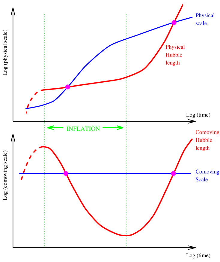
Figure 2: Two equivalent views of how scales evolve during inflation, as compared to the Hubble length which sets the scale of causality. The comoving picture is more transparent, when one recalls that inflation is defined as an epoch where the comoving Hubble length is decreasing. Scales of interest to us today begin much smaller than the Hubble length, where quantum fluctuations are acquired, and by the end of inflation have become much larger than the Hubble length.

III Inflationary models I

In the simplest scenarios, which have been widely explored (see Ref.LLKCBA and references therein), inflation is driven by the potential energy of a single scalar field $\phi$. This potential energy $V(\phi)$, possibly accompanied by a specific mechanism to end inflation, is the model input, and physical observables will be determined by the value of $V$ and its derivatives at the time when those scales cross outside the Hubble radius during inflation. In the simplest models this is the only epoch which matters; before then the scale is well within the Hubble radius and the effect of expansion is negligible, while afterwards the scale is too large to be influenced by causal processes. However, we will see later that this is true only of this simplest class of models.

As far as perturbations are concerned, the simplest models have the following characteristics.

1. As there is only one type of matter, isocurvature perturbations cannot be supported and scalar perturbations must be adiabatic. I’ll call their spectrum $\delta_{{\rm H}}(k)$ (see Ref. LL for a formal definition), where $k$ is the comoving wavenumber.

2. Gravitational waves are always present at some level, and I’ll write their spectrum as $A_{{\rm G}}(k)$. In many models, especially those of the currently-popular hybrid type (see Ref. LR for a thorough review of inflationary model building) they in fact turn out to be negligible.

3. The two spectra can normally be approximated as power-laws

   $$\delta_{{\rm H}}^{2}(k)\propto k^{n-1}\quad;\quad A_{{\rm G}}^{2}(k)\propto k^{n_{{\rm G}}}$$ (4)

   where $n$ and $n_{{\rm G}}$ are the spectral indices and are readily calculated in a given inflation model. However, the power-law expansions are only valid if the inflationary potential is flat enough (see later), and if the available observations are of sufficiently poor quality. High-quality observations make higher accuracy demands on the description of the initial power spectrum.

4. The relative importance of density perturbations and gravitational waves $r$ (measured in terms of their contribution to large-angle microwave background anisotropies) is also readily predicted, and equals approximately $-2\pi n_{{\rm G}}$. In general $n$ and $r$ are independent.

IV Parameters and their determination

From reading some parts of the literature, one might form the impression that the cosmological parameters, such as the Hubble parameter and the density of the Universe, are directly inscribed on the last-scattering surface and hence available to be measured in a model-independent way. Nothing could be further from the truth; the cosmological parameters govern the dynamics of perturbations, and a single time-slice in isolation can say nothing whatsoever about their values. To obtain them, one needs to understand the perturbations at some other epoch, and since this is not accessible to direct observation this initial form must be fixed by assumption. Since there is no unique model supplying these initial conditions, they must be parametrized in some way and those parameters added into the melting pot. The various parameters can be divided into the cosmological parameters (whose role is to describe the present state of the Universe) and the inflationary parameters, describing the initial conditions. A typical set might be

Cosmological parameters

$h$:   

The Hubble parameter.

$\Omega_{0}$:  

The density of matter in the Universe.

$\Lambda$:   

A cosmological constant, if present.

$\Omega_{{\rm B}}$:  

The amount of baryonic matter.

$\Omega_{{\rm HDM}}$:

The amount of hot dark matter, if present.
 (It is assumed that there is always some cold dark matter.)

$\tau$:   

The optical depth to the last scattering surface caused by reionization.

Inflationary parameters

$\delta_{{\rm H}}$: 

The overall amplitude of density perturbations.

$n$:  

The spectral index of the density perturbations.

$r$:  

The effect of gravitational waves on COBE.

Amongst those cosmological parameters, some might be thrown out by assumption; for example we may restrict ourselves to a flat Universe without a hot dark matter component. Typically authors have considered fairly wide cosmological parameter sets. However on the inflationary side most efforts have been very minimal, often with just $\delta_{{\rm H}}$ and $n$ considered. While it might be highly desirable to imagine that the initial conditions can be parametrized by so few parameters, and while indeed that may well in the end turn out to be true, it needs to be acknowledged that less kind circumstances might also prevail, as described in the next section.

Having decided your parameters, you can do two things. The first, which has received quite a bit of attention, is to make estimates of how accurately one can expect to measure said parameters, under the assumption that they provide a sufficient set and for some chosen experimental configuration parest . An example will be given next section. The second thing is to actually go ahead and try and estimate the parameters from some data. This has begun to be popular paramest , though so far the only attempt to cover enough parameters that one can argue they are sufficient is a recent attempt by Tegmark hercules to constrain a nine-parameter space based on the simplest inflation models. Current data is not really up to the task of seriously limiting such a wide parameter volume, but hopefully that will change in the medium future.

V Inflationary models II

The simplest inflationary models are the ones most commonly described. But there are several other possibilities already in the literature, which would impact on the simple picture outlined so far.

• There may be only one field, but with a potential energy $V(\phi)$ which is less flat than we might like.
  Then the power-law approximation might break down. The simplest manifestation of this is for the spectral index $n$ to become scale-dependent, but perhaps amenable to a perturbative approach as outlined later in this section. More drastic is the case of ‘designer’ power spectra, where the potential has sharp features leading to similarly sharp features in the spectra. This would need to be dealt with on a model-by-model basis.

• There may be more than one field.
  Then the adiabatic perturbations might be accompanied by isocurvature perturbations. Superhorizon adiabatic perturbations are then no longer constant modes . We cannot necessarily ignore details of physics while modes are superhorizon, e.g. the (p)reheating epoch which brings inflation to an end.

• Quantum tunnelling effects might be important.
  Then the Universe might be open instead of flat openinf .

I will briefly look at the possible impact of the first two of these.

V.1 Scale-dependent spectral index

The better the quality of observations available, the more likely it is that the power-law approximation is inadequate. It is in fact the beginning of a Taylor expansion of the power spectrum of the form cgl

$$\ln\delta_{{\rm H}}^{2}(k)=\ln\delta_{{\rm H}}(k_{0})+(n-1)\ln\frac{k}{k_{0}}+\frac{1}{2}\left.\frac{dn}{d\ln k}\right|_{k_{0}}\,\ln^{2}\frac{k}{k_{0}}+\cdots\,,$$ (5)

where only the first two terms are kept. The expansion scale $k_{0}$ is arbitrary, but a specific choice is in fact favoured in that it can be chosen so that the estimated errors on $n$ and on $dn/d\ln k$ are uncorrelated.

A perturbative approach is therefore suggested where we add further terms to this series (i.e. adding the coefficients to the parameter estimation process) until a satisfactory fit is achieved. In a given inflation model these coefficients are as easily estimated as $n$ itself, and indeed some inflation models, especially the so-called ‘running mass’ models runmass , can indeed give an effect large enough to be detectable cgl .

When more parameters are added, in principle the error on all parameters is increased. We computed the effect in Ref. cgl , assuming a version of the cold dark matter model and observations by a version of the Planck satellite including polarized detectors, and the table shows how the uncertainties change as extra derivatives of $n$ are added. In fact the picture is quite encouraging. The uncertainties on the cosmological parameters hardly increase at all, and even the uncertainty on the spectral index itself suffers little as extra derivatives are incorporated. It is quite possible therefore that in these models one might get extra information on the inflationary model, through determination of the higher derivatives, while suffering little cost elsewhere.

Table 1: Estimated uncertainty in parameter estimation from measurements by a version of the Planck satellite with polarized detectors. Full details in Ref. cgl .

Parameter		Planck with polarization
$\delta\Omega_{{\rm b}}h^{2}/\Omega_{{\rm b}}h^{2}$		$0.007$	$0.008$	$0.009$
$\delta h/h$		$0.01$	$0.01$	$0.01$
$\delta\Omega_{{\rm\Lambda}}h^{2}/h^{2}$		$0.04$	$0.04$	$0.05$
$\delta\tau$		$0.002$	$0.002$	$0.002$
$\delta n$		$0.004$	$0.004$	$0.006$
$\delta r$		$0.04$	$0.04$	$0.04$
$dn/d\ln k$		$-$	$0.009$	$0.01$
$d^{2}n/d(\ln k)^{2}$		$-$	$-$	$0.02$

V.2 Isocurvature models

If there are multiple scalar fields, then we may find isocurvature perturbations as well as adiabatic ones. This represents a significant complication, because adiabatic and isocurvature modes can source each other even on superhorizon scales if there are interactions between the field or fluid components. Predicting the perturbations in such models presents no problem of principle, but extra information might need to be provided (details of the reheating period ending inflation, for example), whereas in the single field model causality provides a direct bridge from the inflationary era until the scales re-enter the horizon. In general very complicated post-inflation processing between isocurvature and adiabatic modes might occur Hu .

One type of model aims to create only isocurvature perturbations iso . The basic idea is that during inflation, the field which later becomes the CDM already exists and experiences perturbations via the usual quantum fluctuation mechanism. When it later becomes dynamically significant, we have an isocurvature perturbation between CDM and the rest.

Alternatively, there may be a mixture of the two. Low-level isocurvature contamination can impact on parameter estimation, since it will contribute either as a detectable component requiring extra parameters for its description, or as an extra undetectable noise contribution.

Inflationary models of these types have to be compared to observational data on a model-by-model basis. This potentially leads to a wide range of predictions. There is however one saving grace, which is that at least all these models share one characteristic which seems unavoidable, being the existence of a peak structure in the microwave anisotropy spectrum huwhite . This appears to be a generic prediction, as it follows from a simple argument. Because perturbations are established well outside the horizon, they are observed entirely in the growing mode. This necessarily leads to a phase coherence and ultimately to an acoustic peak structure.

The conclusion therefore is that if the observed spectrum fails to feature a series of peaks when measured at high resolution, then inflation cannot be the sole source of perturbations originating structure. Note that phrase carefully however to avoid confusion. If a peak structure is not observed, that doesn’t completely rule out inflation, because it may partly contribute to the anisotropies, an example being the mixed inflation plus defects scenario where the peak structure vanishes if the defects are sufficiently dominant chm . Further, if the peak structure is observed, that does not ‘prove’ inflation. It would support inflation as it would have passed a further observational hurdle, but other mechanisms may be able to produce similar structures.

VI Conclusions

The main point I have aimed to stress in this article is that the inflationary paradigm is a broad one, realizable in a number of ways. The inflationary input is crucial to current views on parameter estimation, not just of the inflationary parameters but the cosmological ons too. If the simplest inflationary models prove correct, all will be well but we will learn only a limited amount about the inflationary mechanism. More desirable would be something a little more complicated, allowing us to extract further information about inflation at only a very modest cost to the cosmological parameters. But we had better hope that the model is not so complicated that it requires so many additional parameters as to have a serious effect on our ability to fit the observational data, or even worse a model which defies parametrization at all. Fortunately, all the current indications are favourable.

References

- (1) A. H. Guth, Phys. Rev. D 23, 347 91981); A. D. Linde, Particle Physics and Cosmology (Harwood, Chur, Switzerland, 1990).
- (2) A. R. Liddle and D. H. Lyth, Phys. Rep. 231, 1 (1993).
- (3) A. Vilenkin and E. P. S. Shellard, Cosmic Strings and Other Topological Defects (Cambridge University Press, 1994).
- (4) U.-L. Pen, U. Seljak and N. Turok, Phys. Rev. Lett. 79, 1611 91997); B. Allen, R. R. Caldwell, S. Dodelson, L. Knox, E. P. S. Shellard and A. Stebbins, Phys. Rev. Lett. 79, 2624 (1997).
- (5) L. Knox, Phys. Rev. D 52, 4307 (1995); G. Jungman, M. Kamionkowski, A. Kosowsky and D. N. Spergel, Phys. Rev. D 54, 1332 (1996); J. R. Bond, G. Efstathiou and M. Tegmark, Mon. Not. R. Astron. Soc. 291, L33 (1997); M. Zaldarriaga, D. Spergel and U. Seljak, Astrophys. J. 488, 1 (1997).
- (6) J. E. Lidsey, A. R. Liddle, E. W. Kolb, E. J. Copeland, T. Barreiro and M. Abney, Rev. Mod. Phys. 69, 373 (1997).
- (7) D. H. Lyth and A. Riotto, to appear, Phys. Rep., hep-ph/9807278.
- (8) K. Ganga, B. Ratra and N. Sugiyama N., Astrophys. J. 461, L61 (1996); M. White and J. Silk, Phys. Rev. Lett. 77, 4704 (1996); J. R. Bond and A. H. Jaffe, in ‘Microwave Background Anisotropies’, ed F. R. Bouchet et al., Editions Frontiéres, astro-ph/9610091; C. H. Lineweaver, D. Barbosa, A. Blanchard and J. G. Bartlett, Astron. Astrophys. 322, 365 (1997); S. Hancock, G. Rocha, A. N. Lasenby and C. M. Gutierrez, preprint astro-ph/9708254 (1998).
- (9) M. Tegmark, preprint astro-ph/9809201 (1998).
- (10) A. A. Starobinsky and J. Yokoyama, in Fourth Workshop on General Relativity and Gravitation, ed K. Nakao et al, astro-ph/9502002 91995); M. Sasaki and E. D. Stewart, Prog. Theor. Phys. 95, 71 (1996); J. garcía-Bellido and D. Wands, Phys.Rev. D 53, 5437 (1996).
- (11) J. R. Gott, Nature 295, 304 (1982); M. Sasaki, T. Tanaka, K. Yamamoto and J. Yokoyama, Phys. Lett. B 317, 510 (1993); M. Bucher, A. S. Goldhaber and N. Turok, Phys. Rev. D 52, 3314 (1995); S. W. Hawking and N. Turok, Phys. Lett. B 425, 25 (1998).
- (12) E. J. Copeland, I. J. Grivell and A. R. Liddle, Mon. Not. R. Astron. Soc. 298, 1233 (1998).
- (13) E. D. Stewart, Phys. Lett. B 391, 34 (1997); E. D. Stewart, Phys. Rev. D 56, 2019 (1997); L. Covi and D. H. Lyth, preprint hep-ph/9809562 (1998).
- (14) W. Hu, preprint astro-ph/9809142 (1998).
- (15) A. D. Linde, Phys. Lett. B 158, 375 (1985); L. Kofman, Phys. Lett. B 173, 400 (1986); A. D. Linde and V. Mukhanov, Phys. Rev. D 56, 535 (1997); P. J. E. Peebles, preprint astro-ph/9805194 (1998).
- (16) W. Hu and M. White, Phys. Rev. Lett. 77 1687 (1996).
- (17) C. Contaldi, M. Hindmarsh and J. Magueijo, preprint astro-ph/9809053 (1998); R. A. Battye and J. Weller, preprint astro-ph/9810203 (1998).