Dust and Extinction Curves in Galaxies with z$>$0:
The Interstellar Medium of Gravitational Lens Galaxies

Abstract

We determine 37 differential extinctions in 23 gravitational lens galaxies over the range $0\mathrel{\raise 1.29167pt\hbox{$<$}\mkern-14.0mu\lower 2.58334pt\hbox{$\sim$}}z_{l}\mathrel{\raise 1.29167pt\hbox{$<$}\mkern-14.0mu\lower 2.58334pt\hbox{$\sim$}}1$. Only 7 of the 23 systems have spectral differences consistent with no differential extinction. The median differential extinction for the optically-selected (radio-selected) subsample is $\Delta E(B-V)=0.04$ ($0.06$) mag. The extinction is patchy and shows no correlation with impact parameter. The median total extinction of the bluest images is $E(B-V)=0.08$ mag, although the total extinction distribution is dominated by the uncertainties in the intrinsic colors of quasars. The directly measured extinction distributions are consistent with the mean extinction estimated by comparing the statistics of quasar and radio lens surveys, thereby confirming the need for extinction corrections when using the statistics of lensed quasars to estimate the cosmological model. A disjoint subsample of two face-on, radio-selected spiral lenses shows both high differential and total extinctions, but standard dust-to-gas ratios combined with the observed molecular gas column densities overpredict the amount of extinction by factors of 2–5. For several systems we can estimate the extinction law, ranging from $R_{V}=1.5\pm 0.2$ for a $z_{l}=0.96$ elliptical, to $R_{V}=7.2\pm 0.1$ for a $z_{l}=0.68$ spiral. For the four radio lenses where we can construct non-parametric extinction curves we find no evidence for gray dust over the IR–UV wavelength range. The dust can be used to estimate lens redshifts with reasonable accuracy, although we sometimes find two degenerate redshift solutions.

1 Introduction

Corrections for extinction have significant cosmological consequences for determining the Hubble constant (e.g. Freedman et al. 1998), the cosmological model using either Type Ia supernovae (Perlmutter et al. 1997, Riess et al. 1998) or gravitational lenses (Kochanek 1996, Falco, Kochanek & Muñoz 1998), and the epoch of star formation (e.g. Madau, Pozetti & Dickinson 1998). Yet detailed, quantitative studies of extinction are largely limited to galaxies closer than $\mathrel{\raise 1.29167pt\hbox{$<$}\mkern-14.0mu\lower 2.58334pt\hbox{$\sim$}}10$ Mpc where it is possible to study individual stars. Studies of extinction at larger distances rely on analyzing the spectral energy distributions of stars mixed with dust, and the amount of dust inferred for a given change in color depends strongly on geometric and other assumptions (e.g. Witt, Thronson & Capuano 1992). The patchy mixture of stars, dust and star forming regions in nearby galaxies illustrates the complexities.

The extinction curves which determine the relation between changes in color and total absorption are reliably measured only in the Galaxy, the LMC and the SMC (see Mathis 1990, Fitzpatrick 1998). We will describe extinction laws by $R_{\lambda}$, where the magnitude change at wavelength $\lambda$ for extinction $E(B-V)$ is $A_{\lambda}=R_{\lambda}E(B-V)$. Most, but not all (Mathis & Cardelli 1992), of the extinction curve variations seen in these three galaxies can be described by parametric functions of the value in the V band, $R_{V}$ (e.g. Savage & Mathis 1979, Fitzpatrick & Massa 1988, Cardelli et al. 1989, Fitzpatrick 1998). The variations tend to be associated with colder, denser regions of the interstellar medium, frequently in directions with appreciable molecular gas (e.g. Jenniskens & Grennberg 1993). The variations affect mainly the optical and ultraviolet extinction curve. The infrared and near-infrared extinction curve is a fixed power law with $R_{\lambda}\propto\lambda^{-\alpha}$ and $\alpha\simeq 1.7\pm 0.1$ (Mathis 1990). In the Galaxy, typical paths with modest total extinctions have $R_{V}\simeq 3.1$, while paths through denser, higher extinction regions can reach an $R_{V}>5$ for an overall range of $2.2\mathrel{\raise 1.29167pt\hbox{$<$}\mkern-14.0mu\lower 2.58334pt\hbox{$\sim$}}R_{V}\mathrel{\raise 1.29167pt\hbox{$<$}\mkern-14.0mu\lower 2.58334pt\hbox{$\sim$}}5.8$. The changes in the optical extinction curve are correlated with the width and amplitude of the 2175Å PAH feature. In the SMC and a few regions of the LMC, however, the ultraviolet extinction curve differs significantly from the standard Galactic law with the same optical extinction properties. The principal difference is that these regions have a far weaker 2175Å feature (e.g. Gordon & Clayton 1998). Physically, the extinction law depends on the mean size and composition distribution of the dust grains along the line of sight (e.g. Draine & Malhotra 1993, Rouleau, Henning & Stognienko 1997), so it is not surprising that the properties of the extinction curve depend on the environment.

The Galaxy, the LMC, and the SMC do not constitute a representative sample of galaxy types, ages, metallicities, or star formation histories, and the available data on extinction curves in other galaxies provide little evidence that the typical extinction law observed in the Galaxy is also typical for other galaxies. Estimates in M31 produce a range of $3.5$ to $5.3$ for $R_{V}$ where the variations appear to be linked to the local metallicity (Walterbos 1986, Hodge & Kennicutt 1982, Iye & Richter 1985). There is some evidence that extinction curves in early-type galaxies are significantly steeper as a function of $\lambda^{-1}$, with $1.9\mathrel{\raise 1.29167pt\hbox{$<$}\mkern-14.0mu\lower 2.58334pt\hbox{$\sim$}}R_{V}\mathrel{\raise 1.29167pt\hbox{$<$}\mkern-14.0mu\lower 2.58334pt\hbox{$\sim$}}2.8$ (e.g. Warren-Smith & Berry 1983, Rifatto 1990, Brosch & Loinger 1991, Goudfrooij et al. 1994). Lower $R_{V}$ values correspond to a smaller average size for the dust grains compared to the Galaxy. Riess, Press & Kirshner (1996) estimated a mean extinction curve $R_{V}=2.55\pm 0.30$ for 20 nearby Type Ia supernovae with I, R, V and B band photometry, which is marginally consistent with the typical Galactic value. Despite the observed variations in the extinction curve, the typical Galactic or extreme SMC extinction curves are almost universally adopted for all other galaxies from $z=0$ to $z>5$. Extinction curves almost certainly evolve with redshift since the metallicity, elemental abundance ratios, mean star formation rate, and energy injection rates which determine the structure and evolution of the dust are all strong functions of redshift.

Recently, two new techniques for making direct measurements of dust in high redshift galaxies have appeared. The first new method is simply an extension of local methods for stars to the far brighter Type Ia supernovae (Riess et al. 1998, Perlmutter et al. 1997). Accurate extinction measurements and corrections are essential to the goal of using the Type Ia supernovae to determine the cosmological model. The second new method is to use multiply imaged gravitational lenses. As first pointed out by Nadeau et al. (1991), the lenses can be used to determine the differential extinction between the images and the extinction law in the lens galaxy. Jean & Surdej (1998) noted that it is also possible to determine the redshift of the dust in systems with significant differential extinction. Malhotra, Rhoads & Turner (1997) attempted the first survey of extinction in lenses based on the overall optical and infrared colors of the systems, concluding that many lens galaxies had large, uniform dust opacities. However, high resolution imaging has now shown that many of the radio lenses with red broad band colors are red because the flux from the source is dominated by light from the AGN host galaxy (see Kochanek et al. 1998b).

The Center for Astrophysics/University of Arizona Space Telescope Lens Survey (CASTLES) is systematically obtaining V, I and H band photometry of the nearly $50$ known lens systems. The broad wavelength coverage makes accurate determinations of the extinction in point-source lens systems relatively simple. The substantial number of lenses with extended optical and infrared sources are more difficult to use; we will ignore them for the current survey. By combining our CASTLES data with archival HST and ground-based photometry we can perform a preliminary survey of extinction in 23 gravitational lenses, 8 of which were radio-selected. Unlike the optically-selected systems, the radio-selected systems should be unbiased with respect to the dust content of the lens galaxy. In §2 we describe the method for determining extinctions and extinction laws. In §3 and §4 we determine the differential and total extinctions for the systems assuming a standard $R_{V}=3.1$ Galactic extinction law. In §5 we estimate extinction laws and dust redshifts. In §6 we discuss the implications of our results for determining the cosmological model using gravitational lens statistics and Type Ia supernovae. We summarize our results and discuss future expansions of the method in §7.

2 Methods

For a gravitational lens, we can divide the study of extinction into determining the differential extinction between the lines of sight traversed by the images through the galaxy, and the total extinction along the lines of sight. The differential extinction is the more easily and accurately measured because it requires only the assumption that the spectrum of the source is identical for each of the images. The total extinction is more difficult to determine because it depends on a model for the intrinsic spectrum of the source and combines extinction from the Galaxy, the lens, and the host.

We observe $N_{i}$ lensed images of a point-source whose intrinsic spectrum expressed in magnitudes at an observed wavelength $\lambda$ and time $t$ is $m_{0}(\lambda,t)$. The images we see at time $t$ are magnified by $M_{i}(\lambda,t)$ and have time delays $\Delta t_{i}$, so that the observed spectrum of image $i$ at time $t$ is

$$m_{i}(\lambda,t)=m_{0}({\lambda\over 1+z_{s}},t-\Delta t_{i})-2.5\log M_{i}({\lambda\over 1+z_{l}},t)+E_{i}R_{i}({\lambda\over 1+z_{l}})+E_{Gal}R_{Gal}(\lambda)+E_{src}R_{src}({\lambda\over 1+z_{s}})$$ (1)

where $E_{i}$, $E_{Gal}$ and $E_{src}$ are the extinctions $E(B-V)$ due to the lens for image $i$, the Galaxy respectively, and the source’s host galaxy, and $R_{i}(\lambda)$, $R_{Gal}(\lambda)$, and $R_{src}(\lambda)$ are the extinction laws for the lens at image $i$, the Galaxy, and the host galaxy respectively. The lens and host extinction curves must be redshifted by the lens and host redshifts $z_{l}$ and $z_{s}$. The images pass through the lens at locations separated by kpc, so we expect different extinctions and possibly even different extinction laws for each of the images. The ray separations in the host galaxy or our Galaxy are so small ($\sim 10^{-5}d\ll 1$ pc for dust at distance $d<1$ kpc from the source or observer) that we can safely assume that the host and the Galaxy contribute equal extinctions to all images. If (1) the magnification is wavelength independent; (2) the magnification is time independent; (3) the source spectrum is time independent for the both the duration of the observations and the time delays; and (4) the extinction curves for the images are identical, then the magnitude differences between images $i$ and $j$,

$$m_{i}(\lambda)-m_{j}(\lambda)=-2.5\log{M_{i}\over M_{j}}+(E_{i}-E_{j})R\left({\lambda\over 1+z_{l}}\right),$$ (2)

depend only on the constant magnification ratios $M_{i}/M_{j}$, the extinction differences $E_{i}-E_{j}$, and the extinction curve $R(\lambda/(1+z_{l}))$ in the lens rest frame. Nadeau et al. (1991) were the first to explore the dependence of the flux ratios on the extinction and the extinction curve, while Jean & Surdej (1998) pointed out the potential utility of the dependence on the lens redshift. For a lens with $N_{im}=2$ or $4$ images with flux ratios measured at $N_{\lambda}$ wavelengths we have $(N_{im}-1)N_{\lambda}$ constraints to determine $N_{im}-1$ flux ratios and differential extinctions when the extinction law is fixed. Two wavelengths are sufficient for a measurement, but three are needed to check the consistency of the solution. For an extinction curve parameterized by $R_{V}$, we need measurements at three or more wavelengths to estimate $R_{V}$. We can also determine the extinction curve non-parametrically (following Nadeau et al. 1991). For a two-image lens we can determine the curve at $N_{\lambda}-2$ wavelengths, but we will always find a perfect fit to the data and there will be no degrees of freedom left to check the solution. Four-image systems are better because the multiple lines-of-sight add considerable redundancy. Radio data are particularly valuable because we can be certain that they are completely unaffected by dust, allowing us to detect, limit or rule out dust which is gray over the entire IR–UV wavelength range.

We estimate the differential extinctions by fitting the measured magnitude differences assuming no time dependence to the spectrum, wavelength dependence for the magnification, or position dependence to the extinction law. Thus, we minimize

$$\chi^{2}=\sum_{j=1}^{N_{\lambda}}\sum_{i=1}^{N_{im}}{\left(m_{i}(\lambda_{j})-m_{0}(\lambda_{j})-2.5\log M_{i}-E_{i}R(\lambda_{j}/(1+z_{l}))\right)^{2}\over\sigma_{ij}^{2}+\sigma_{sys}^{2}}$$ (3)

over the $i=1\cdots N_{im}$ images and $j=1\cdots N_{\lambda}$ filters for magnitude measurements $m_{i}(\lambda_{j})$ with uncertainties $\sigma_{ij}$. We include an additional systematic error term $\sigma_{sys}$ whose value is set to zero for the actual fits. We simply used the standard central wavelengths of the filters in the calculations. We set one magnification to unity and one extinction to zero because we can only measure relative magnifications and differential extinctions. We always picked the bluest (i.e. lowest-extinction) image to be the reference for the extinction.

The general expression in eqn. (1) illustrates the possible limitations of the method. The two most important are time variability and gravitational microlensing. Time variability affects the results through the time delay differences $\Delta t_{i}$ between the images. If the data to be modeled are collected at a single epoch, then only variations in the shape of the spectrum affect the extinction results, while if we combine data from multiple epochs both changes in the total flux and the spectral shape affect the extinction results. When time variability is observed in quasars and AGN, it is seen at all wavelengths simultaneously (e.g. Ulrich, Maraschi & Megan 1997, Neugebauer et al. 1989), so the changes in the overall flux are generally larger than the changes in the spectral shape. While the mean magnification of the lens is constant and achromatic, gravitational microlensing introduces both temporal variations and chromaticity (see Schneider, Ehlers & Falco 1992). The radio emitting, optical broad/narrow line, and accretion disk regions have different physical sizes and thus can have different average magnifications (see Schneider, Ehlers & Falco 1992). Where variability is observed in lenses it is seen at all wavelengths simultaneously (e.g. Kundić et al. 1997, Corrigan et al. (1991), Ostensen et al. (1996)) and in both the continuum and the strong emission lines (Saust 1994). Time variability in the mean magnification is more common and has a larger amplitude than chromatic variations.

The systematic errors will broaden the extinction distributions beyond the effects of purely statistical errors, distort extinction curve estimates, and bias redshift estimates. The $\chi^{2}$ values of the fit provide a simple means of estimating the level of systematic errors. If our ansatz that the spectral differences between the images are due only to differential magnification and extinction is correct, then we should find solutions with $\chi^{2}\simeq N_{dof}\pm(2N_{dof})^{1/2}$ where $N_{dof}$ is the number of degrees of freedom. If we find a poor statistical fit, then the true magnitude errors produced by the unmodeled systematic uncertainties (time variability and microlensing) should be of order $(\chi^{2}/N_{dof})^{1/2}$ larger than the statistical errors in the magnitudes. Once the parameters of the fit were determined, we found the value for the systematic error parameter $\sigma_{sys}$ which would produce $\chi^{2}=N_{dof}$ as an estimate of the level of systematic error required to invalidate the procedure.

The determination of the total extinction is a more dangerous procedure. We will assume that all sources have an intrinsic spectrum which can be modeled by the mean spectrum of bright optically-selected quasars. We produced a composite UV-IR quasar spectrum including the dominant emission lines by combining the UV-IR continuum model of Elvis et al. (1994) with the mean spectrum including broad emission lines of Francis et al. (1991). We computed the intrinsic colors of the quasar by convolving the redshifted mean spectrum with the appropriate filter functions. By including only lenses dominated by point sources, we avoid the systematic error in Malhotra et al. (1997) of interpreting the red colors of extended emission from the source’s host galaxy as reddened emission by a quasar (see Kochanek et al. 1998b, King et al. 1998). It is known, however, that the broad range of colors observed for unlensed, radio-selected quasars is not exclusively due to contamination by emission from the host galaxy (see Masci, Webster & Francis 1998). The red colors of many radio-selected sources must be due either to extinction of the AGN by the host galaxy (e.g. Wills et al. 1992) or intrinsic differences in the AGN spectrum (e.g. Impey & Neugebauer 1988). Thus, for the radio-selected lenses we will frequently over-estimate the total extinction in the lens galaxy because our assumption for the intrinsic spectrum is either invalid or represents a determination of the amount of dust in the host galaxy.

We first estimated an upper bound to the extinction from the requirement that the source have an intrinsic magnitude fainter than $M_{B}=-29$ mag ($H_{0}=50$ km s^-1 Mpc^-1). Brighter quasars are exceedingly rare at all redshifts (e.g. Hartwick & Schade 1990). While we will not include a correction, an offset would lead to a increase in our total extinction estimates by the same amount. We estimated the limit using the bluest image and bluest filter to the red of Ly$\alpha$. We used a constant lens magnification correction of a factor of 10 – using the true magnifications will have only a modest effect on the limits. Next we estimated the total extinction from the color of the bluest image on the longest available wavelength base-line to the red of Ly$\alpha$. If we call the red filter $r$ and the blue filter $b$ at observed wavelengths $\lambda_{r}$ and $\lambda_{b}$, then

$$r-b=(r-b)_{0}(z_{s})+E_{Gal}(R(\lambda_{b})-R(\lambda_{r}))+E_{lens}(R({\lambda_{b}\over 1+z_{l}})-R({\lambda_{r}\over 1+z_{l}}))+E_{src}(R({\lambda_{b}\over 1+z_{s}})-R({\lambda_{r}\over 1+z_{s}}))$$ (4)

where $E_{Gal}$, $E_{lens}$ and $E_{src}$ are the $E(B-V)$ contributions from the Galaxy, the lens and the source respectively. We assume a fixed $R_{V}=3.1$ Galactic extinction law for all three components, and corrected the individual lenses for Galactic extinction using the model of Schlegel, Finkbeiner & Davis (1998). The intrinsic color $(r-b)_{0}(z_{s})$ was derived by redshifting the mean quasar spectrum and convolving it with the appropriate filter passbands. The uncertainties in the colors and extinctions are entirely systematic. The spectral index of the optical continuum of quasars ($F_{\nu}\propto\nu^{\alpha}$) is $\alpha\simeq-0.4\pm 0.6$ (Francis et al. 1991), which would lead to an uncertainty in the extinction of $\sigma_{E}\simeq\sigma_{\alpha}/3\simeq 0.2$ mag for typical wavelength baselines and lens redshifts if it also characterized the uncertainties in the optical through infrared continuum. We determine the extinction errors scaled to an uncertainty in the intrinsic color of $\sigma_{r-b}=0.1$ mag, and then estimate the accuracy of the error estimates from the distribution of extinctions. Since we have no means of separately determining $E_{lens}$ and $E_{src}$ given the uncertainties in the intrinsic spectrum, we have estimated $E_{lens}$ with $E_{src}\equiv 0$. For red radio quasars created by dust in their host galaxy we will mistakenly assign $E_{src}$ to $E_{lens}$, and for intrinsically red radio quasars we will produce nonsense.

3 Differential Extinction Estimates for $R_{V}=3.1$

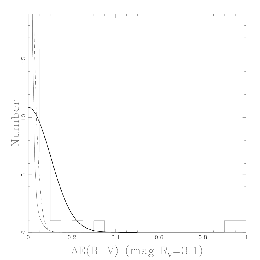
Figure 1: Histogram of the differential extinction for $R_{V}\equiv 3.1$. Only values with standard errors smaller than $\sigma(E(B-V))<0.1$ mag are included. The highest extinction lens (PKS 1830–211) is shown in the rightmost bin, but actually has a higher extinction (see Table 2). The light solid curve shows the distribution expected due to random photometric errors based on the standard errors of the individual $E(B-V)$. The light dashed curve shows the expected distribution due to random photometric errors after rescaling the errors by $(\chi^{2}/N_{dof})^{1/2}$ when $\chi^{2}>N_{dof}$ to compensate for underestimated photometric uncertainties. The light solid and dashed curves exclude the high differential extinction lenses B 0218+357 and PKS 1830–211 because their large absolute (but small fractional) errors are not relevant for the reliability of the small differential extinction measurements. The heavy solid curve is the the best fit Gaussian model for the differential extinctions excluding B 0218+357 and PKS 1830–211.

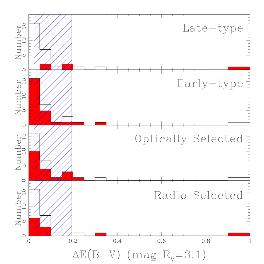
Figure 2: Histograms of differential extinction estimates by subsample. The shaded histograms show (from bottom to top) the distributions for radio-selected, optically-selected, early-type and late-type lenses. The unshaded histogram superposed on each of the panels shows the overall distribution from Figure 1. Galaxies with unknown morphologies have been added to the early-type sample. The hatched region shows the estimated range for the mean total extinction in lens galaxies estimated from a comparison of optically-selected and radio-selected lens statistics by Falco et al. (1998).

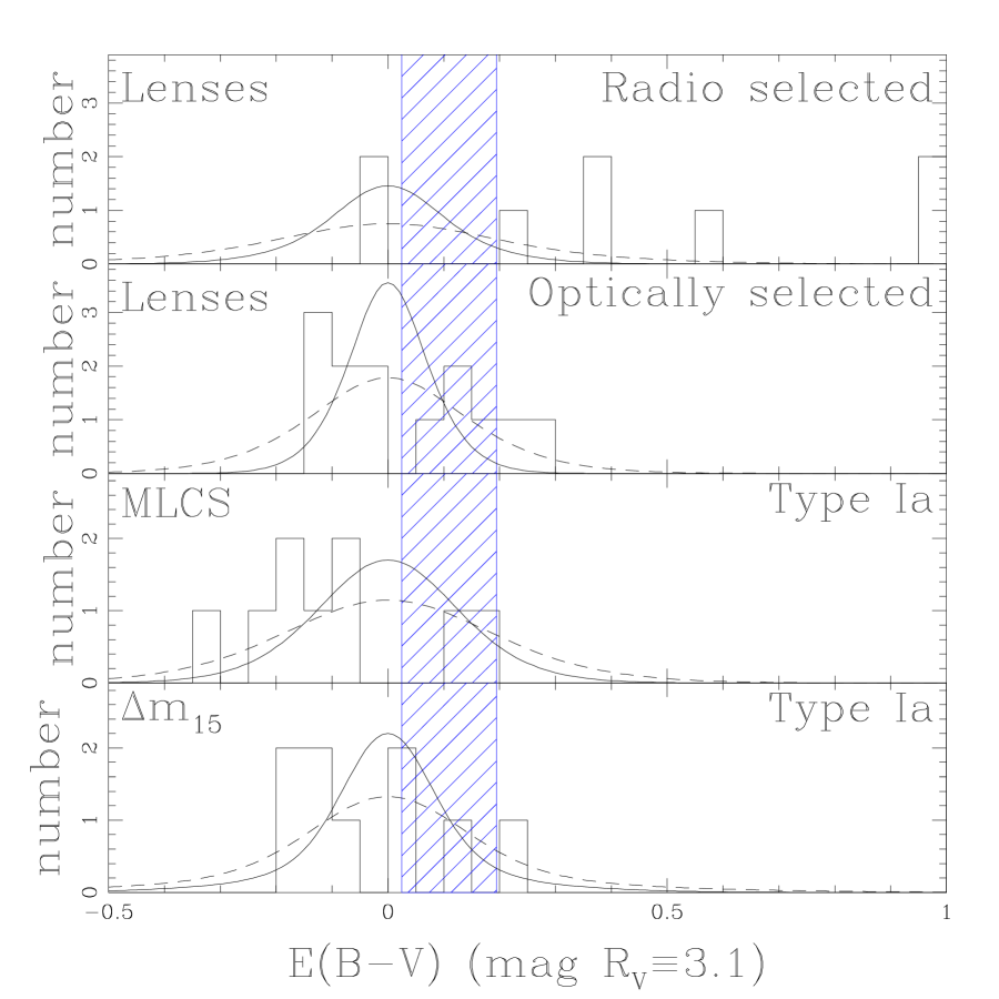
Figure 3: Histograms of total extinction. The top histograms show the total extinction distributions for the bluest images of the radio-selected and optically-selected subsamples. The bottom two histograms show the distribution of Type Ia supernova extinctions from Riess et al. (1998) using either the MLCS or $\Delta m_{15}$ analysis methods. The solid curves show the extinction distributions expected from random errors given the nominal extinction uncertainties. The dashed curves show the distributions expected after broadening the nominal uncertainties by a factor of 2 for the lenses, 1.5 for the MLCS method, and 1.7 for the $\Delta m_{15}$ method.

We start by estimating the differential extinctions in the lenses because these can be determined independently and more accurately than the total extinctions. Differential extinction estimates have been made for many individual lens systems (e.g. McLeod et al. (1998) most recently for MG 0414+0534, Hewett et al. (1994) for LBQS 1009–0252, Chae & Turnshek (1998) most recently for H 1413+117, Nadeau et al. (1991) for Q 2237+0305), but here we present the first full, systematic survey. We selected 23 lens systems with multiply imaged point-sources. Of the 23 systems, 8 were radio-selected (12 differential extinctions) and 15 were optically-selected (25 differential extinctions). We have fewer radio-selected than optically-selected systems because so many of the radio lenses are dominated by extended sources for which our analysis procedure does not apply. The exclusion of systems because their sources are extended is unbiased with respect to the extinction in the lens galaxy. Where the lens redshifts are unknown, we have used preliminary redshift estimates from the fundamental plane of lens galaxies (Kochanek et al. 1998a). Modest errors in the redshift estimates ($\Delta z\mathrel{\raise 1.29167pt\hbox{$<$}\mkern-14.0mu\lower 2.58334pt\hbox{$\sim$}}0.2$) will not significantly alter the distribution of differential extinctions. The data we used in the analysis are presented in Table 1.

We first fit each of the systems using eqn. (3) and assuming no differential extinction. Table 2 presents the $\chi^{2}_{1}$ statistic for the fits to each system. We find that 7 of the 23 systems are consistent with no differential extinction or any other systematic difference between the spectral shapes of the images. Next we fit the systems assuming a $R_{V}=3.1$ Cardelli et al. (1989) parameterized extinction curve. All the initially poorly fit systems show dramatic improvements in their goodness of fits. Note, however, that only 10 of the 23 systems have $\chi^{2}_{2}$ statistics consistent with a good fit ($\chi^{2}_{2}\simeq N_{dof}$). The poor fits can be explained by underestimated photometric errors (generally by a factor of $\sim 2$), systematic errors in the extinction calculation (using the wrong extinction curve or lens redshift), or systematic errors due to unrelated physics (spectral variability and microlensing). We attempt to compensate our quantitative estimates for systematic errors by rescaling the uncertainties in the extinction or intrinsic flux ratios by the factor $(\chi^{2}_{2}/N_{dof})^{1/2}$ whenever $\chi^{2}_{2}>N_{dof}$. The procedure is equivalent to broadening the photometric uncertainties so that the best fit model has $\chi^{2}_{2}=N_{dof}$, or to redoing the fits with a non-zero value for $\sigma_{sys}$.

The resulting estimates for the differential extinctions and the intrinsic flux ratios of the images are presented in Tables 3 and 4 using the rescaled uncertainties. Figure 1 presents the distribution of differential extinctions $\Delta E(B-V)$ for the overall sample after dropping the two lenses (HST 12531–2914 and HST 14176+5226) where the standard error in the estimate exceeds $\sigma(\Delta E(B-V))>0.1$ mag. Photometric errors would produce a distribution of non-zero extinctions even in the absence of dust. We can estimate this “null” distribution by the normalized sum of one-sided Gaussians for each measurement (excluding B 0218+357 and PKS 1830–211 whose large errors absolute but small fractional errors are not relevant to the null distribution), leading to the very narrow distribution contained within the first bin of Figure 1. If we use the rescaled errors instead of the original errors, the null distribution is broader but still significantly narrower than the observed distribution. Thus, the differential extinction distribution is only marginally broadened by the effects of photometric uncertainties. If we fit the distribution of differential extinctions excluding B 0218+357 and PKS 1830–211 with a Gaussian broadened by either the standard or rescaled statistical error estimates we find a best fit width for the distribution of $\sigma_{\Delta E}=0.1$ mag, which is roughly consistent with the observed median of $0.05$ mag (see Figure 1).

Figure 2 presents the extinction distributions for two different ways of dividing the data into subsamples. The first division is into radio-selected and optically-selected lenses, where the first is unbiased and the second is biased with respect to the amount of extinction. The second division is into early-type and late-type lenses. Four of the lenses (the optically-selected lens Q 2237+0305, and the radio-selected lenses B 0218+357, B 1600+434, PKS 1830–211) are late-type galaxies based on morphology, color, or molecular gas content. Most lenses are early-type galaxies which lie on the fundamental plane (Kochanek et al. 1998a) with the the expected colors, sizes and morphologies (Keeton et al. 1998). Since most lenses are expected to be early-types, we have put the currently unclassified lenses (SBS 0909+532, LBQS 1009–0252, Q 1017–207, Q 1208+1011, and H 1413+117) into the early-type subsample. It is not surprising that the two highest-extinction systems, B 0218+357 and PKS 1830–211, are both radio-selected systems and have late-type lens galaxies. Both are nearly face-on, cover the quasar images, have exponential rather than early-type photometric profiles (Lehár et al. 1999) and contain large amounts of molecular gas (see §4). The other two late-type galaxies lie amidst the main lens population. For Q 2237+0305 we see the images through the bulge rather than the disk of the galaxy, and for B 1600+434 the images lie on either side of the edge-on lens galaxy. The median extinction of the optically-selected subsample of $\Delta E(B-V)=0.04$ mag is slightly smaller than the median extinction of the radio-selected sample of $\Delta E(B-V)=0.06$ mag, as might be expected given the bias against dusty systems in the optical samples.

In the four-image systems the images usually all lie at a common distance from the lens center, while in the two-image systems the images usually lie at significantly different distances from the image center. We find no pattern in the extinction as a function of impact parameter relative to the lens center. In half of the lenses the inner image is more reddened and for the other half of the lenses the outer image is more reddened. For example, the inner image of B 0218+357 passes $0\farcs 1$ from the lens center and the outer image passes $0\farcs 2$ from the lens center, but the outer image shows $\Delta E(B-V)=0.9$ mag more extinction than the inner image. Thus, the dust distribution in the lens galaxies must be patchy, just as in nearby galaxies.

4 Estimates of the Total Extinction for $R_{V}=3.1$ and the Dust-to-Gas Ratio

We discuss the estimates of the total extinction separately because the need to assume an intrinsic color for the quasars makes the results less reliable than the estimates for the differential extinction. The estimates of total extinction are also presented in Table 3, along with the upper bound on the rest-frame $A_{V}$ above which the source luminosity exceeds that of the brightest known quasars. In most cases the extinction estimated from the image colors is significantly below the physical limit set by the maximum quasar luminosities. The median total extinction of the bluest images is $E(B-V)=0.08$ mag. We can also estimate the typical total extinction of the lens systems by comparing the statistics of radio and optical lens surveys. If we normalize the statistical models using the radio surveys, then we can use the optical surveys to estimate the mean extinction needed to reconcile the two samples. Falco et al. (1998) performed such a comparison and found $\langle A_{B}\rangle\simeq 0.58\pm 0.45$ mag in the observers rest frame. For a typical lens redshift of $z_{l}\simeq 0.5$ the B band extinction coefficient at the lens is $R_{QSO}\simeq 6$ and thus the mean extinction is $\langle E(B-V)\rangle\simeq\langle A_{B}\rangle/R_{QSO}\simeq 0.10\pm 0.08$ mag. The estimated median total extinction for the individual lenses agrees with the extinction estimated from the statistical comparison.

Figure 3 shows the extinction distributions for the blue images divided into radio-selected and optically-selected subsamples. The superposed curves show the distribution predicted from random errors in the intrinsic source color using either the standard error ($\sigma_{r-b}=0.1$ mag) or twice the standard error. The absence of a broader tail of negative extinctions means that our standard error estimate is approximately correct, and that we are at most underestimating the uncertainties by a factor of two. Even so, much of the total extinction distribution, particularly for the optically-selected subsample, is dominated by the uncertainties in the intrinsic colors. We also see no correlation between the differential and total extinctions for the low total extinction lenses ($E(B-V)\mathrel{\raise 1.29167pt\hbox{$<$}\mkern-14.0mu\lower 2.58334pt\hbox{$\sim$}}0.2$ mag), which is probably a sign that the distribution is dominated by noise.

It is clear that the distribution of the radio-selected lenses differs from that of the optically-selected lenses. We know that radio-selected quasars have a broader range of colors than optically-selected quasars (e.g. Webster et al. 1995), and that contamination from the host galaxy can be only a partial explanation (e.g. Masci et al. 1998). In the two high differential extinction lenses, B 0218+357 and PKS 1830–211, it is likely that the total extinctions of $E(B-V)=0.6$ mag can be attributed to dust in the lens. On the other hand, MG 0414+0534 has the highest total extinction estimate for the blue image ($E(B-V)=1.4$ mag or 5 times the largest differential extinction in the system) but the extinction is probably due to dust in the source. A model using only dust in the lens must explain why there are $<20\%$ variations in the extinction across a region spanning $13h_{65}^{-1}$ kpc, and that the arc image of the quasar host galaxy is significantly bluer than the quasar images (Falco et al. 1998). The intrinsic spectra of galaxies are redder than those of optically-selected quasars, so the only way to find a blue arc and a red quasar is to put the dust in the source. Dust in the lens would produce a red quasar and a still redder arc. Moreover, the inferred intrinsic luminosity of the arc is $\sim 0.5L_{*}$ without any extinction correction, so adding $A_{B}=6$ mag of dust in the lens is implausible. We found a similar situation in the lens MG 1131+0456 (Kochanek et al. 1998b), where the lens galaxy is demonstrably transparent but dust in the host galaxy obscures the AGN cores. Thus, the broad range of extinctions estimated for the radio-lenses is problematic.

Absorption by HI and molecular gas in the lens galaxy is seen in two systems, B 0218+357 and PKS 1830–211. For these systems we can use our direct estimates of the extinction to determine the dust-to-gas ratios of the lens galaxies. In both systems the molecular and atomic absorption is seen in front of only one image. In B 0218+357 the molecular gas at $z_{l}=0.69$ is seen in front of the A image (Menten & Reid 1996). In PKS 1830–211 the molecular gas at $z_{l}=0.89$ is seen in front of the B (Southwest) image (Frye, Welch & Broadhurst 1997), and there may be HI absorption at $z=0.19$ in front of the A (Northeast) image (Lovell et al. 1996). The molecular absorption is inferred to be in optically thick CO clouds which incompletely cover the continuum radio source. For B 0218+357 the H₂ column density estimates range from $N(H_{2})\simeq 2\times 10^{22}$ cm^-2 (Wiklind & Combes 1995, Gerin et al. 1997) to $5\times 10^{23}$ cm^-2 (Wiklind & Combes 1995, Combes & Wiklind 1997), combined with an HI column density of $N(HI)\simeq 10^{21}$ cm^-2 (Carilli, Rupen & Yanny 1993). For PKS 1830–211 the H₂ column density in front of the B image is estimated to be $N(H_{2})\simeq 2.5\times 10^{22}$ cm^-2 (Wiklind & Combes 1996, 1998, Gerin et al. 1997), and the HI column density in front of the A image is estimated to be $N(HI)\simeq 10^{20}$ cm^-2. X-ray spectra of PKS 1830–211 show a deficit of soft X-rays compared to normal quasar X-ray spectral indices, which could be explained by a gas density in the lens of $N(H)\simeq 3.5\times 10^{22}$ covering both images (Mathur & Nair 1997).

For both lenses, standard conversions of gas surface density to extinction (e.g. $A_{V}\simeq 6.3\times 10^{-22}\left[N(HI)+2N(H_{2})\right]$, Savage et al. 1977)) predict total extinctions of $A_{V}\mathrel{\raise 1.29167pt\hbox{$>$}\mkern-14.0mu\lower 2.58334pt\hbox{$\sim$}}20$ mag. Such an estimate is patently wrong, because for $A_{V}\mathrel{\raise 1.29167pt\hbox{$>$}\mkern-14.0mu\lower 2.58334pt\hbox{$\sim$}}20$ the quasars would be unphysically luminous. The luminosity limit of $M_{B}>-29$ mag sets an upper bound to the total extinction of the blue image of $A_{V}<3.5$ for B 0218+357 and $A_{V}<4.1$ for PKS 1830–211. The extinction estimates for B 0218+357 are $A_{VA}=4.7$ mag and $A_{VB}=1.9$ mag, corresponding to molecular column densities of $N(H_{2})\simeq 4\times 10^{21}$ cm^-2 and $2\times 10^{21}$ cm^-2 respectively. The extinction estimates for PKS 1830–211 are $A_{VA}=1.8$ mag and $A_{VB}=11.1$ mag respectively, corresponding to molecular column densities of $N(H_{2})\simeq 1\times 10^{21}$ cm^-2 and $9\times 10^{21}$ cm ^-2 respectively. In both cases, either the dust-to-gas ratio is a factor of 2–5 times lower than standard estimates, or the optical source coincidentally lies behinds one of the gaps in the molecular gas coverage. The low extinction of the PKS 1830–211 A image probably means that there is little X-ray absorption by the lens at the A image and that Galactic absorption must be largely responsible for suppressing the soft X-rays. The high $R_{V}$ extinction curves that best fit the two lenses (see §5) alter the differential component of $A_{V}$ from $2.8$ to $3.5$ mag for B 0218+357 and from $9.3$ to $7.2$ mag for PKS 1830-211, which is insufficient to explain the apparent change in the dust-to-gas ratio.

5 Extinction Laws and Lens Redshifts

Determining extinction laws (Nadeau et al. 1991) and lens redshifts (Jean & Surdej 1998) is more difficult than determining extinctions because they are more sensitive to the systematic errors introduced by variability and microlensing. The current data are not ideal because the wavelength coverage is usually limited to the V band and redder filters, and because we are forced to combine data from epochs spanning a period of several years. The results of this section should be regarded more as a feasibility study rather than a final, complete survey. In particular, the reliability would be considerably increased if the data were obtained at a common epoch. Note, however, that we are again using only the spectral differences between the images and avoid the uncertainties about the intrinsic spectrum.

We first found the best fit value of $R_{V}$ for the Cardelli et al. (1989) parameterized extinction curves using fixed lens redshifts and a prior probability of $R_{V}=3.1\pm 1.0$ on the extinction law. We adopt the prior to stabilize the results when the data are inadequate to determine $R_{V}$. Table 3 presents the goodness of fit, $\chi^{2}_{3}/N_{dof}$, and the estimated value of $R_{V}$. We can divide the systems into three loose categories. The first group consists of the seven lenses with small differential extinctions ($\Delta E(B-V)<0.04$ mag, Q 0142–100, BRI 0952–0115, Q 0957+561, Q 1017–207, B 1030+074, PG 1115+080, HE 2149–2745) and the two lenses with large fractional uncertainties in the differential extinction (HST 12531–2914, HST 14176+5226). For these systems the extinction curve is either poorly determined or overly subject to small systematic errors. For example, Q 0957+561 has little extinction ($\Delta E(B-V)=0.02\pm 0.02$ mag for $R_{V}=3.1$), but we derive a value of $R_{V}=7.7\pm 0.9$. The large change in the $\Delta\chi^{2}$ between fixed and variable $R_{V}$ is almost certainly due to using photometric uncertainties which are underestimates of the true uncertainties (i.e. $\sigma_{sys}>0$). The second group consists of SBS 0909+532 and B 1600+434 for which we derive $R_{V}<1$. We believe these are unphysical and the result of problems in the data. The SBS 0909+532 photometry is mainly from ground-based observations that may be significantly contaminated by the lens galaxy, while the optical and radio flux ratios for B 1600+434 are poorly determined and variable.

The third group consists of the 12 systems with plausible $R_{V}$ estimates. Seven are consistent with $R_{V}=3.1$ given the uncertainties (LBQS 1009–0252, HE 1104–1805, Q 1208+1011, H 1413+117, B 1422+231, SBS 1520+530 and MG 2016+112) and five are not (B 0218+357, MG 0414+0534, FBQ 0951–0115, PKS 1830–211 and Q 2237+0305). However, for none of the systems consistent with $R_{V}=3.1$ can the existing data significantly reduce the uncertainties beyond the level specified by the prior. Added data can improve little the results for H 1413+117 and B 1422+231 where the differential extinctions are fairly low and there is good wavelength coverage in the existing data. The other systems have larger extinctions and poorer wavelength coverage so the prospects for significantly reducing the extinction curve uncertainties are good. Of the five with atypical values of $R_{V}$, three are variable (B 0218+357–Biggs et al. 1998 (radio), Wagner 1998 (IR); PKS 1830–211–Lovell et al. 1998 (radio); Q 2237+0305–Corrigan et al. 1991, Ostensen et al. 1996 (optical)), and one is not variable (MG 0414+0534–Moore & Hewitt 1997 (radio), Schechter 1998 (optical)). There are no variability data on FBQ 0951–0115 or IR–UV variability data for PKS 1830–211.

For B 0218+357, MG 0414+0534, MG 2016+112 and Q 2237+0305 we can derive non-parametric extinction curve estimates with sufficiently small formal uncertainties to compare to the parametric determinations. Figure 4 shows the standard ($R_{V}=3.1$) and best fit parametric models along with the non-parametric model. The non-parametric extinction curves match the best fit parametric curves given the formal uncertainties for three of the systems, while for MG 2016+112 there is a discrepant point associated with the Gunn r band photometry. Note that distinguishing the best fit extinction curve from the typical Galactic $R_{V}=3.1$ curve depends almost entirely on the data to the blue of the rest frame V band. With only data to the red of the rest frame V band, the self-similarity of the extinction curve makes it almost impossible to distinguish the models. All four lenses are radio sources, so the agreement of the non-parametric and parametric models rules out the existence of a significant gray dust opacity over the IR–UV wavelength range. The high $R_{V}$ extinction curves are, however, relatively gray compared to the standard $R_{V}=3.1$ curve.

Three of the four systems have significantly non-standard extinction curves, so we need to demonstrate that the results are due to extinction rather than systematic error. One test is to show that the extinction curve is not varying with time. For example, the Q 2237+0305 curve includes time averaged ground-based light curves at V, R and I from Ostensen et al. (1996) covering epochs from 1990 to 1995 as well as the V and R HST observations from 1995 and 1990 respectively. We processed the data as separate points in the extinction curve and found that the $R_{\lambda}$ values derived from the ground-based and HST data agree given their mutual uncertainties. Note, however, that if we include the earlier Corrigan et al. (1991) ground-based photometric data, we obtain discordant results for the extinction curve. Whether this is an artifact of variability or a consequence of the more sophisticated image modeling approach of Ostensen et al. (1996) over Corrigan et al. (1991) is unclear.

Figure 4: Extinction curves for B 0218+357 (top left), MG 0414+0534 (top right), MG 2016+112 (bottom left) and Q 2237+0305 (bottom right). The solid line shows the standard $R_{V}=3.1$ curve and the dashed line shows the best fit parametric curve. For simplicity the curves are normalized by the $R_{\lambda}$ value of the filter closest to the lens rest frame V band. All four lenses are radio sources and include a point at $\lambda^{-1}=0$, allowing an absolute determination of both the extinction and the extinction curve. For MG 0414+0534 the heavy dashed line is an $R_{V}=1.5$ extinction curve at the true lens redshift of $z_{l}=0.96$, while the light dashed line is the better fitting $R_{V}=2.1$ extinction curve at $z_{l}=0.23$, thereby illustrating the dust redshift degeneracy.

Figure 5: A comparison of spectroscopic and dust redshifts. The redshift uncertainties were determined by the region with $\Delta\chi^{2}=1$ from the minimum. The filled points are the primary (deepest) minima, and the open points are secondary minima in the $\chi^{2}$ surface. Figure 4 shows the similarity of the two best fit extinction curve-redshift solutions for MG 0414+0534.

Next, for the systems where the extinction curve was determinable at a single redshift we attempted to estimate the redshift and the extinction law simultaneously. Four problems potentially limit the determination of dust redshifts. First, the extinction law in the IR and NIR is almost self-similar, $R_{\lambda}\propto\lambda^{1.7\pm 0.1}$, and only the deviations from self-similarity permit a redshift determination. Second, lines of sight in the Galaxy with the same value of $R_{V}$ do not have exactly identical extinction curves (e.g. Mathis & Cardelli 1992). The value of $R_{V}$ is the most important parameter of the extinction curve, but it is not the only parameter. Third, the largest deviations from self-similarity occur in the UV and are associated with the behavior of the 2175Å bump. However, it is the structure of the UV extinction curve that varies the most between the Galaxy and the SMC. Fourth, at some level the lensing data must be contaminated by microlensing and the resulting wavelength dependence of the magnification. These systematic errors will be far more important for dust redshift determinations, which depend on the small deviations from a self-similar extinction curve, than for estimates of $E(B-V)$. Thus, estimates of the accuracy of dust redshifts based on Monte Carlo simulations of photometric errors, as considered by Jean & Surdej (1998), are likely to underestimate the true uncertainties. We will take a purely empirical approach, and determine the dust redshifts for every system with adequate data and then compare the known and estimated redshifts.

In Table 5 we present the dust redshift estimates for all lenses with $E(B-V)>0.05$ mag and standard errors $\sigma(E(B-V))<0.1$ mag for $R_{V}=3.1$. We also included B 1422+231 which has slightly less extinction because the lens redshift is known and can be compared to the dust redshift. Of the 12 lenses, three yielded no good redshift estimate (SBS 0909+532, HE 1104–1805, and SBS 1520+530) in the sense that the redshift range covered by the standard errors in the redshift estimate were too large ($\Delta z_{dust}>0.5$). Four of the lenses had two minima in the $\chi^{2}(z_{s})$ curve, and we present both solutions for the redshift. Figure 5 compares the dust redshifts and their standard errors for the six lenses which also have spectroscopic redshifts (B 0218+357, MG 0414+0534, B 1422+231, B 1600+434, MG 2016+112 and Q 2237+0305). In four cases the primary (deepest) minimum is close to the true redshift, and in two cases it is not. MG 0414+0534, B 1600+434 and MG 2016+112 have both primary and secondary solutions, one of which lies near the true lens redshift. Note, however, that the primary minimum for MG 0414+0534 lies near $z_{dust}=0.20$ instead of the true lens redshift of $z_{l}=0.96$ with $\Delta\chi^{2}=7.1$ (some of the difference is due to the the prior on $R_{V}$). The high and low redshift solutions have extraordinarily similar extinction curves (see the MG 0414+0534 panel of Figure 4), and the relative probability of the two solutions is controlled by the systematic uncertainties in the flux ratios and the extinction curve. It is clear that simple Gaussian statistics based on the photometric errors are not a reliable means of discriminating between primary and secondary minima. We find a dust redshift consistent with the true redshift for five of the six cases in the sense that $|z_{dust}-z_{l}|$ is either consistent with the (Gaussian) uncertainties or exceeds an absolute accuracy of $|z_{dust}-z_{l}|<0.1$. The exception is B 1422+231, which has the least extinction of the twelve. If we drop B 1422+231 for having insufficient extinction and consider only the correct minima, the absolute accuracy of the dust redshifts is good, with $\langle z_{dust}-z_{l}\rangle=0.00\pm 0.08$. The formal redshift uncertainties are reasonable for MG 0414+0534, B 1600+434 and MG 2016+112, but are clearly underestimates for Q 2237+0305 and B 0218+357. In summary, dust redshift estimates for lenses with sufficient differential extinction appear to accurately determine the lens redshift, but can produce multiple, degenerate solutions that cannot be safely distinguished using simple Gaussian statistics.

6 Consequences for Cosmology

Estimates of the cosmological model using both gravitational lenses and Type Ia supernovae are very sensitive to extinction. For optically selected gravitational lens samples, extinction reduces the amount of magnification bias (see Kochanek 1996), and for supernovae it increases the inferred distance modulus in the standard fashion. For both methods, the inferred matter density is underestimated by approximately $\Delta\Omega\simeq-A_{B}$ in magnitudes for flat cosmological models.

Falco et al. (1998) estimated the mean effects of extinction by comparing the statistics of optically-selected quasar and radio lens samples. They found that the two samples could be reconciled if the mean extinction of a lensed quasar was $\langle A_{B}\rangle\simeq 0.6\pm 0.4$ mag or $E(B-V)\simeq 0.10\pm 0.08$ mag. As we discussed in §3 and §4 and illustrated in Figures 2 and 3, the directly observed lens extinction distributions are consistent with the statistical estimates. In Figure 6 we illustrate the changes in the probability of finding a lensed quasar for several simple models of the extinction distributions. We simplified the calculations by fixing the conversion from $E(B-V)$ to $A_{B}$ in the observer’s frame to that for a lens at $z_{l}=0.5$ with an $R_{V}=3.1$ extinction curve. Otherwise the calculations follow those of Kochanek (1996). We first considered analytic models using a two-sided Gaussian distribution of differential extinctions (i.e. no correlation between impact parameter and extinction) of width $\sigma_{\Delta E}$ and a one-sided Gaussian distribution of total extinctions of width $\sigma_{E}$. In §3 we found that $\sigma_{\Delta E}\simeq 0.1$ mag excluding the two high differential extinction lenses, and in §4 we found that the median total extinction was $0.08$ mag. The total extinction estimate is inaccurate because of the large uncertainties in the intrinsic source colors. We also simply use the measured extinctions as a model of the distribution, without any corrections for the broadening of the distribution by measurement errors other than to reset the negative total extinctions to be zero. We made the calculation using either the differential or the combined total and differential extinction distributions for either the radio or optically selected lenses.

Small amounts of differential extinction have little effect on the statistics (see Figure 6). A Gaussian differential extinction distribution with $\sigma_{\Delta E}=0.1$ mag lowers the expected number of lensed quasars by about 20%. We get the same result if we use the observed differential extinction distribution for the optically-selected lens sample. If we use the differential extinction distribution of the radio-selected lens sample, the expected number of lenses drops by 25–35% because of the two radio lenses with high differential extinctions which were not included in the Gaussian model. The total extinction has a much stronger effect on the lens probabilities – for $\sigma_{E}=0.1$ mag the expected number of lenses drops by 40–60% if $\sigma_{\Delta E}=0.1$ mag and by 30–50% if $\sigma_{\Delta E}=0.05$ mag. Similarly, the number of lenses drops by 40–50% if we use the observed total and differential extinctions for the optically-selected sample, and by 80% if we use the distribution for the radio lenses. The 80% drop is inconsistent with the Falco et al. (1998) comparison of the statistics of the two types of lens samples, and it provides further evidence that the intrinsic colors of radio sources are different from those of bright optically-selected quasars.

Figure 6: Effects of extinction on the probability of lensing quasars. The histogram shows the magnitude distribution of quasars surveyed for gravitational lenses from Kochanek (1996). The solid curves show the ratio of the probability of lensing with dust to that without dust as a function of quasar magnitude for four analytic models. In the analytic models (solid curves) the dust is characterized by the dispersions of the (one-sided) Gaussian distributions for the extinction of the bluest image, $\sigma_{E}$, and the differential extinction $\sigma_{\Delta E}$. In the empirical models (dashed curves) we use the observed distributions for the radio (R) and optical (O) samples using either only the differential extinction (R$\Delta$, O$\Delta$) or both the total and differential extinctions (R, O). Negative total extinctions were simply set to zero, and no corrections are made for broadening of the distribution by photometric errors.

The lens galaxies lie at redshifts comparable to those of the host galaxies of the Type Ia supernovae used by Riess et al. (1998) and Perlmutter et al. (1997) to determine the cosmological model. The impact parameters of the lensed images are also comparable to those of the supernovae. Thus, the extinctions seen in the lens galaxies must to some extent be comparable to those expected for the supernovae. The two samples are not, however, identical. The lenses accurately determine the extinction differences and poorly determine the total extinction on paths passing completely through the lens galaxy, while the supernovae are sensitive only to the total foreground extinction. The lens galaxies are dominated by massive, metal-rich, early-type galaxies, while the supernovae host galaxies are typically lower mass, lower metallicity, late-type galaxies. Later type hosts would imply more dust, lower metallicity would imply less dust, and total foreground extinction rather than differential extinction could imply either more or less dust.

We can make three qualitative statements about what should be observed for the supernovae given the results for extinction in gravitational lenses. First, we clearly find evidence for patchy extinction in both early-type and late-type galaxies at similar redshifts and impact parameters to the supernova sample. Even though the two samples cannot be trivially compared, it would be surprising for the supernova sample to show markedly less extinction than the lens sample. Second, from the 4 lenses for which we can derive non-parametric extinction curves, we find no evidence for gray dust at optical wavelengths. This eliminates one potential, if physically unlikely, source of systematic uncertainty for the supernova projects. Note, however, that the high $R_{V}$ extinction curves are quite gray compared to the typical $R_{V}=3.1$ curve. Third, we find additional evidence that extinction curves are not universal and can deviate significantly from “standard” Galactic dust even in regions of low total extinction. The uncertainty in the appropriate extinction curve must be regarded as a source of systematic uncertainty. Since dust grain distributions depend on the history of dust production and destruction, which in turn depends heavily on the metallicity and the mean star formation and energy injection rates, it would be surprising if the “typical” extinction curve did not evolve with redshift.

In Figure 3 we compare the total extinction estimates for the bluest lens images to the raw extinction estimates for the Type Ia supernovae in Riess et al. (1998). We could not compare to the Perlmutter et al. (1997) sample because they did not estimate extinctions. As with the estimates of the total extinctions of the gravitational lenses, the intrinsic colors of the supernovae are too poorly constrained to allow accurate individual extinction estimates. The extinction distribution of the supernovae is peculiar because 11 of the 15 extinction estimates are negative. Figure 3 also shows the expected distribution of extinctions given the uncertainty estimates for the individual measurements using either the MLCS (typical $\sigma_{E}=0.13$ mag) or $\Delta m_{15}$ (typical $\sigma_{e}=0.10$ mag) analysis methods. In both cases, the distribution of the measurements is significantly broader than the model, and simple statistical tests show that the distribution of supernova extinctions is inconsistent with the stated uncertainties and random errors even if all supernovae had zero intrinsic extinction at a slightly greater than 2-$\sigma$ confidence level. The best fit to the observed extinction distribution requires that the true uncertainties in the extinction be $\sigma_{E}\simeq 0.18$ mag and that the MLCS and $\Delta m_{15}$ methods underestimate the true uncertainties by a factors of 1.5 and $1.7$ respectively.

There are four possible interpretations of the inconsistency. First, it may be genuine sample variance. However, the 2-$\sigma$ confidence level for the existence of the inconsistency was derived without the inclusion of the 5 “snapshot” supernovae, which also show a preponderance of negative extinctions. Second, the Type Ia fitting methods are underestimating errors by a factor of 1.5–1.7. The covariance between extinction and distance means that we must rescale the distance errors by the same factor as the extinction errors. The rescaling has serious cosmological consequences because for 50% larger errors, a 2-$\sigma$ confidence region in the $\Omega_{0}$–$\Lambda_{0}$ plane becomes a less than 1-$\sigma$ confidence region. Third, an estimate of zero extinction in the supernova sample may not really be zero. The Type Ia extinction estimates are actually differential measurements relative to supernovae in nearby ellipticals which are defined to have zero extinction. If these systems have non-zero extinction due to diffuse dust such as we appear to see in many of the lenses, then the true zero-point of the supernovae extinction scale might be somewhat negative. In this case the existing cosmological limits are biased towards high $\Omega_{0}$ (low $\Lambda_{0}$) by the Bayesian procedure for renormalizing negative extinctions. Fourth, there may be a systematic error or evolutionary effect making the high redshift supernovae systematically bluer than the low redshift comparison samples. Which of these solutions is correct will only become apparent in larger samples, but it is clear that the derivation of a physical, self-consistent extinction distribution for the supernovae is a powerful test of the assumptions and uncertainty estimates used in the supernova cosmology programs.

7 Summary

We measured 37 extinctions in 23 gravitational lenses, which constitutes the largest set of direct extinction measurements outside the local universe. We can accurately measure small differential extinctions ($|\Delta E(B-V)|\mathrel{\raise 1.29167pt\hbox{$>$}\mkern-14.0mu\lower 2.58334pt\hbox{$\sim$}}0.02$ mag) or large absolute extinctions ($E(B-V)\mathrel{\raise 1.29167pt\hbox{$>$}\mkern-14.0mu\lower 2.58334pt\hbox{$\sim$}}0.1$ mag) because the former depends only on observed spectral differences while the latter requires a model for the intrinsic spectrum. The median differential extinctions of $\Delta E(B-V)=0.04$ ($0.06$) mag for optically (radio) selected lenses are modest. There are two exceptions, both of which are face-on, gas-rich spiral lenses with differential extinctions of $\Delta E(B-V)=0.9$ and $3.0$ mag respectively. We see no pattern of lensed images at small impact parameters showing systematically higher extinctions than those at large impact parameters. If we assume a model for the intrinsic color of the quasars based on the composite quasar spectra of Elvis et al. (1994) and Francis et al. (1991) we can estimate the total extinction. We find a median total extinction for the bluest images of $E(B-V)=0.08$ mag, but the distribution is dominated by the uncertainties in the intrinsic colors of the quasars and AGN. The similarity of the mean and differential extinctions and the lack of a correlation between image radius and extinction suggests that the interstellar medium of the lenses is patchy. For most lenses, the spectral differences cannot be fully explained by extinction using a parametric extinction curve and the measured photometric errors – deviations from the parametric law, systematic underestimates of the photometric errors, time variability, and microlensing must contribute to the spectral differences.

Most lens galaxies are early-type galaxies based on their colors, morphologies, luminosities (Keeton et al. 1998) and they lie on the fundamental plane (Kochanek et al. 1998a). Thus, the lens sample appears to provide unambiguous evidence for patchy, diffuse dust in some early-type galaxies on scales of $\sim 5h_{65}^{-1}$ kpc (1$\farcs$0 at $z=0.5$). There is considerable evidence for dusty disks and patchy dust in the central regions ($<$ 1 kpc) of local early-type galaxies (e.g. Schweizer 1987, Kormendy & Stauffer 1987, Goudfrooij et al. 1994, van Dokkum & Franx 1995). In fact, van Dokkum & Franx estimate that 80% of ellipticals contain nuclear dust once corrections are made for the difficulty of detecting face-on dusty disks. The amount of dust on the larger scales (1–5 kpc) typical of the impact parameters of the lensed images is less clear in the local samples, but Goudfrooij & de Jong (1995) argue for the existence of a diffuse dust component with $0.04\mathrel{\raise 1.29167pt\hbox{$<$}\mkern-14.0mu\lower 2.58334pt\hbox{$\sim$}}E(B-V)\mathrel{\raise 1.29167pt\hbox{$<$}\mkern-14.0mu\lower 2.58334pt\hbox{$\sim$}}0.25$ to explain the discrepancy between the IRAS flux presumed to arise from dust emission and the mass of patchily distributed dust derived from optical images. Their estimate of a diffuse dust component is consistent with the estimate of $E(B-V)=0.10\pm 0.08$ mag by Falco et al. (1998) from comparisons of optical and radio lens surveys.

The two lenses with the highest differential and mean extinctions, the face-on late-type lenses B 0218+357 and PKS 1830–211, produce molecular and atomic absorption features in the radio and millimeter continuum of the quasar (Carilli et al. 1993, Wiklind & Combes 1995, 1996). The inferred molecular column densities combined with standard dust-to-gas ratios overpredict the amount of extinction by factors of 2–5. No detailed analysis is necessary to realize there is a problem because the standard dust-to-gas ratios predict $A_{V}>20$ mag – such large extinctions would make the sources intrinsically more luminous than any known quasar. For both heavily extincted images we infer an extinction curve with $R_{V}\simeq 6$–$7$ instead of $3.1$, and the properties of the absorbing regions are very similar to those regions of the Galaxy where high $R_{V}$ extinction curves are measured. The remaining good candidate for the detection of molecular absorption lines in the sample is the lensed radio quasar MG 0414+0534 with $z_{l}=0.96$ and $z_{s}=2.64$. We estimate $N(H_{2})\simeq 7\times 10^{20}$ cm^-2 based on the largest differential extinction or $N(H_{2})\mathrel{\raise 1.29167pt\hbox{$>$}\mkern-14.0mu\lower 2.58334pt\hbox{$\sim$}}4\times 10^{21}$ cm^-2 based on the total extinction, although we expect the total extinction to be associated with the source rather than the lens.

For systems with sufficient differential extinction, we can estimate both the extinction law (Nadeau et al. 1991) and the redshift of the dust (Jean & Surdej 1998). Many of the estimated extinction curves do not match the standard Galactic $R_{V}=3.1$ curve. For example, the $z_{l}=0.96$ elliptical lens MG 0414+0531 has $R_{V}=1.5\pm 0.2$ and the $z_{l}=0.68$ spiral lens B 0218+357 has $R_{V}=7.2\pm 0.1$. Dust redshifts appear to work reasonably well provided there is sufficient differential extinction to determine the extinction curve at a fixed redshift accurately. For the systems where the lens redshift is known, the agreement between the spectroscopic and dust redshifts suggests that the derived extinction curves are correct – it is difficult to see how a systematic error can both mimic a deviant extinction curve and select out the true lens redshift. The dust redshifts can be remarkably accurate, with $\langle z_{dust}-z_{l}\rangle=0.00\pm 0.08$, if we confine the comparison to the systems with high differential extinction ($E(B-V)>0.05$ mag for $R_{V}=3.1$) and drop incorrect secondary redshift solutions. However, when there are multiple solutions, the systematic uncertainties in the data and the extinction curve models make it dangerous to choose between the minima based on simple Gaussian statistics.

The extinctions have a significant effect on determinations of the cosmological model from the statistics of lensed quasars and the brightness of Type Ia supernovae. Our directly measured extinction distributions are consistent with the statistical estimates from a comparison of radio-selected and optically-selected lens surveys by Falco et al. (1998). Any cosmological estimate using the statistics of lensed quasars requires a substantial correction for extinction. Both recent attempts to reconcile the statistics of lensed quasars with the results of the Type Ia supernovae surveys (Chiba & Yoshii 1998, Cheng & Krauss 1998) neglected the effects of extinction, thereby producing significant overestimates in the expected number of lensed quasars in any given cosmology. Since we are unable to determine the distribution of total extinctions in the gravitational lenses accurately given the uncertainties in the intrinsic source colors, only the statistics of lensed radio sources can be used to directly estimate the cosmological model using gravitational lens statistics (Falco et al. 1998, Cooray 1998). The statistics of lensed quasars can be used to estimate the cosmological model only after correcting for the total extinction derived from a comparison of the radio and optical lens samples. Extinction determinations for high redshift Type Ia supernovae (Riess et al. 1998, Perlmutter et al. 1997) have similar accuracy problems, which makes it difficult to compare the extinction distributions of the lens and supernova samples. We did find, however, an internal inconsistency at greater than 2-$\sigma$ confidence in the Riess et al. (1998) supernovae extinctions and their uncertainties, whose most obvious symptom is that 75% of the supernovae extinctions are negative. While the origin of the inconsistency is as yet unclear, the derivation of self-consistent, physical extinction distributions for the supernovae is a critical test of the results of the supernova cosmology projects.

The existing lens data were never intended for extinction studies, so there is enormous potential for improvement. Systematic errors can be minimized by obtaining all the necessary multiwavelength photometry at a common epoch. Broader wavelength coverage, particularly the addition of B and U band photometry, would greatly improve the precision of the estimates for the extinction, the extinction curves, and lens redshifts. For many lenses the photometry could be done from the ground because there will be little contamination from the early-type lens galaxies at these wavelengths, although HST is required for the smaller separation systems. The 2175Å dust feature should be detectable for many lenses if their extinction laws resemble that for the Galaxy or the LMC rather than the SMC. The feature is redshifted to more easily observed wavelengths, appearing at $2175(1+z_{l})$Å. Although observable from the ground for lenses with redshifts $z_{l}\mathrel{\raise 1.29167pt\hbox{$>$}\mkern-14.0mu\lower 2.58334pt\hbox{$\sim$}}0.8$, precision spectrophotometry of the closely spaced images or lower redshift lenses will require HST/STIS to detect or limit the presence of the feature.

Table 1: Magnitude Differences

Lens	$\lambda^{-1}$	Image 1	Image 2	Image 3	Image 4	Source
	$\mu$m-1	mag	mag	mag	mag
	$1.48$	$\equiv 0\pm 0.05$	$2.35\pm 0.03$			Lehár et al. (1999)
	$0.63$	$\equiv 0\pm 0.02$	$2.29\pm 0.02$			Lehár et al. (1999)
B0218+357	$2.92$	$\equiv 0\pm 0.20$	$-1.10\pm 0.10$			Lehár et al. (1999)
	$1.80$	$\equiv 0\pm 0.10$	$-2.25\pm 0.03$			Lehár et al. (1999)
	$1.23$	$\equiv 0\pm 0.01$	$-2.40\pm 0.01$			Lehár et al. (1999)
	$0.63$	$\equiv 0\pm 0.01$	$-0.57\pm 0.01$			Lehár et al. (1999)
	$0.00$	$\equiv 0\pm 0.01$	$1.40\pm 0.02$			Patnaik et al. (1995)
MG0414+0534	$1.48$	$\equiv 0\pm 0.03$	$1.18\pm 0.03$	$0.73\pm 0.03$	$1.56\pm 0.04$	CASTLES
	$1.23$	$\equiv 0\pm 0.02$	$0.94\pm 0.02$	$0.81\pm 0.02$	$1.67\pm 0.06$	CASTLES
	$0.91$	$\equiv 0\pm 0.02$	$0.49\pm 0.02$	$0.95\pm 0.02$	$1.78\pm 0.02$	CASTLES
	$0.63$	$\equiv 0\pm 0.03$	$0.32\pm 0.03$	$1.01\pm 0.03$	$1.86\pm 0.03$	CASTLES
	$0.49$	$\equiv 0\pm 0.03$	$0.20\pm 0.03$	$1.04\pm 0.03$	$1.90\pm 0.03$	CASTLES
	$0.00$	$\equiv 0\pm 0.04$	$0.13\pm 0.04$	$1.04\pm 0.04$	$2.09\pm 0.04$	Moore & Hewitt (1997)
SBS0909+532	$2.25$	$\equiv 0\pm 0.04$	$1.29\pm 0.04$			Kochanek et al. (1997)
	$1.52$	$\equiv 0\pm 0.04$	$0.58\pm 0.04$			Kochanek et al. (1997)
	$1.24$	$\equiv 0\pm 0.04$	$0.31\pm 0.04$			Kochanek et al. (1997)
	$0.63$	$\equiv 0\pm 0.01$	$0.13\pm 0.03$			Lehár et al. (1999)
FBQ0951+2635	$2.24$	$\equiv 0\pm 0.03$	$0.89\pm 0.03$			Schechter et al. (1998)
	$1.80$	$\equiv 0\pm 0.03$	$0.94\pm 0.03$			Schechter et al. (1998)
	$1.52$	$\equiv 0\pm 0.03$	$0.96\pm 0.03$			Schechter et al. (1998)
	$1.24$	$\equiv 0\pm 0.03$	$0.95\pm 0.03$			Schechter et al. (1998)
	$0.63$	$\equiv 0\pm 0.02$	$1.36\pm 0.02$			CASTLES
	$0.00$	$\equiv 0\pm 0.04$	$1.67\pm 0.18$			Schechter et al. (1998)
BRI0952-0115	$1.49$	$\equiv 0\pm 0.04$	$1.29\pm 0.03$			Lehár et al. (1999)
	$0.63$	$\equiv 0\pm 0.01$	$1.37\pm 0.01$			Lehár et al. (1999)
Q0957+561	$4.03$	$\equiv 0\pm 0.05$	$0.06\pm 0.05$			Dolan et al. (1995)
	$3.52$	$\equiv 0\pm 0.05$	$0.06\pm 0.05$			Dolan et al. (1995)
	$1.80$	$\equiv 0\pm 0.01$	$0.01\pm 0.02$			Bernstein et al. (1997)
	$1.23$	$\equiv 0\pm 0.02$	$0.02\pm 0.02$			Bernstein et al. (1997)
	$0.63$	$\equiv 0\pm 0.01$	$0.08\pm 0.01$			CASTLES
	$0.00$	$\equiv 0\pm 0.02$	$0.32\pm 0.02$			Conner et al. (1992)
LBQS1009-0252	$2.25$	$\equiv 0\pm 0.14$	$2.52\pm 0.14$			Hewett et al. (1994)
	$1.82$	$\equiv 0\pm 0.07$	$2.62\pm 0.07$			Hewett et al. (1994)
	$1.50$	$\equiv 0\pm 0.07$	$2.26\pm 0.07$			Hewett et al. (1994)
	$1.25$	$\equiv 0\pm 0.06$	$2.03\pm 0.06$			Hewett et al. (1994)
	$0.63$	$\equiv 0\pm 0.02$	$1.58\pm 0.03$			Lehár et al. (1999)
Q1017-207=J03	$1.80$	$\equiv 0\pm 0.02$	$2.16\pm 0.03$			Lehár et al. (1999)
	$1.23$	$\equiv 0\pm 0.02$	$2.15\pm 0.02$			Lehár et al. (1999)
	$0.63$	$\equiv 0\pm 0.03$	$2.15\pm 0.04$			Lehár et al. (1999)
B1030+074	$1.80$	$\equiv 0\pm 0.01$	$3.08\pm 0.04$			Lehár et al. (1999)
	$1.23$	$\equiv 0\pm 0.02$	$3.05\pm 0.09$			Lehár et al. (1999)
	$0.00$	$\equiv 0\pm 0.17$	$2.96\pm 0.17$		Xanthopoulos et al. (1998)
HE1104-1805	$1.80$	$\equiv 0\pm 0.01$	$1.76\pm 0.03$			Lehár et al. (1999)
	$1.23$	$\equiv 0\pm 0.01$	$1.61\pm 0.02$			Lehár et al. (1999)
	$0.63$	$\equiv 0\pm 0.03$	$1.47\pm 0.03$			Lehár et al. (1999)
PG1115+080	$1.80$	$\equiv 0\pm 0.01$	$0.45\pm 0.01$	$1.97\pm 0.01$	$1.47\pm 0.01$	CASTLES
	$1.23$	$\equiv 0\pm 0.02$	$0.39\pm 0.01$	$1.96\pm 0.01$	$1.46\pm 0.02$	CASTLES
	$0.63$	$\equiv 0\pm 0.03$	$0.48\pm 0.03$	$1.93\pm 0.02$	$1.48\pm 0.05$	Impey et al. (1998)
Q1208+1011	$2.28$	$\equiv 0\pm 0.04$	$1.36\pm 0.04$			Bahcall et al. (1992)
	$1.80$	$\equiv 0\pm 0.02$	$1.56\pm 0.02$			Bahcall et al. (1992)
	$1.27$	$\equiv 0\pm 0.02$	$1.51\pm 0.02$			Bahcall et al. (1992)
	$1.42$	$\equiv 0\pm 0.02$	$1.51\pm 0.02$			Bahcall et al. (1992)
	$0.63$	$\equiv 0\pm 0.01$	$1.63\pm 0.01$			Lehár et al. (1999)
HST12531-2914	$1.65$	$\equiv 0\pm 0.15$	$-0.13\pm 0.15$	$-0.30\pm 0.11$	$0.49\pm 0.24$	Ratnatunga et al. (1995)
	$1.23$	$\equiv 0\pm 0.24$	$-0.31\pm 0.17$	$-0.39\pm 0.18$	$-0.08\pm 0.24$	Ratnatunga et al. (1995)
H1413+117	$2.98$	$\equiv 0\pm 0.03$	$0.34\pm 0.02$	$-0.02\pm 0.02$	$0.17\pm 0.03$	Turnshek et al. (1997)
	$2.97$	$\equiv 0\pm 0.02$	$0.28\pm 0.02$	$-0.07\pm 0.02$	$0.21\pm 0.02$	Monier et al. (1998)
	$2.67$	$\equiv 0\pm 0.02$	$0.26\pm 0.02$	$0.05\pm 0.02$	$0.17\pm 0.02$	Monier et al. (1998)
	$2.35$	$\equiv 0\pm 0.02$	$0.23\pm 0.02$	$0.09\pm 0.02$	$0.40\pm 0.02$	Monier et al. (1998)
	$2.12$	$\equiv 0\pm 0.02$	$0.21\pm 0.02$	$0.20\pm 0.02$	$0.21\pm 0.02$	Monier et al. (1998)
	$1.90$	$\equiv 0\pm 0.02$	$0.22\pm 0.02$	$0.20\pm 0.02$	$0.33\pm 0.02$	Monier et al. (1998)
	$1.81$	$\equiv 0\pm 0.05$	$0.17\pm 0.05$	$0.23\pm 0.05$	$0.31\pm 0.05$	Turnshek et al. (1997)
	$1.81$	$\equiv 0\pm 0.04$	$0.23\pm 0.04$	$0.25\pm 0.04$	$0.43\pm 0.04$	Turnshek et al. (1997)
	$1.81$	$\equiv 0\pm 0.09$	$0.31\pm 0.05$	$0.35\pm 0.06$	$0.49\pm 0.06$	Turnshek et al. (1997)
	$1.74$	$\equiv 0\pm 0.02$	$0.20\pm 0.02$	$0.23\pm 0.02$	$0.34\pm 0.02$	Monier et al. (1998)
	$1.60$	$\equiv 0\pm 0.02$	$0.20\pm 0.02$	$0.22\pm 0.02$	$0.31\pm 0.02$	Monier et al. (1998)
	$1.42$	$\equiv 0\pm 0.02$	$0.17\pm 0.03$	$0.31\pm 0.03$	$0.41\pm 0.02$	Turnshek et al. (1997)
	$1.42$	$\equiv 0\pm 0.02$	$0.15\pm 0.02$	$0.28\pm 0.02$	$0.35\pm 0.02$	Turnshek et al. (1997)
	$1.23$	$\equiv 0\pm 0.02$	$0.10\pm 0.02$	$0.30\pm 0.02$	$0.40\pm 0.02$	Turnshek et al. (1997)
	$0.63$	$\equiv 0\pm 0.01$	$0.10\pm 0.01$	$0.38\pm 0.01$	$0.62\pm 0.02$	McLeod et al. (1998)
	$0.00$	$\equiv 0\pm 0.10$	$0.20\pm 0.10$	$0.61\pm 0.10$	$0.53\pm 0.10$	McLeod et al. (1998)
HST14176+5226	$1.65$	$\equiv 0\pm 0.06$	$0.14\pm 0.07$	$0.36\pm 0.08$	$0.34\pm 0.08$	Ratnatunga et al. (1995)
	$1.23$	$\equiv 0\pm 0.08$	$0.26\pm 0.09$	$0.35\pm 0.10$	$0.43\pm 0.12$	Ratnatunga et al. (1995)
B1422+231	$2.92$	$\equiv 0\pm 0.03$	$-0.42\pm 0.03$	$0.26\pm 0.03$	$3.62\pm 0.03$	Impey et al. (1996)
	$2.09$	$\equiv 0\pm 0.02$	$-0.28\pm 0.02$	$0.50\pm 0.02$	$3.68\pm 0.05$	Impey et al. (1996)
	$2.08$	$\equiv 0\pm 0.03$	$-0.25\pm 0.03$	$0.41\pm 0.03$	$3.81\pm 0.03$	Impey et al. (1996)
	$2.03$	$\equiv 0\pm 0.03$	$-0.28\pm 0.03$	$0.52\pm 0.03$	$3.64\pm 0.03$	Yee & Ellingson (1994)
	$1.90$	$\equiv 0\pm 0.02$	$-0.29\pm 0.02$	$0.50\pm 0.02$	$3.72\pm 0.05$	Impey et al. (1996)
	$1.82$	$\equiv 0\pm 0.05$	$-0.25\pm 0.05$	$0.55\pm 0.05$	$3.71\pm 0.10$	Remy et al. (1993)
	$1.74$	$\equiv 0\pm 0.02$	$-0.20\pm 0.02$	$0.57\pm 0.02$	$3.76\pm 0.05$	Impey et al. (1996)
	$1.60$	$\equiv 0\pm 0.02$	$-0.26\pm 0.02$	$0.50\pm 0.02$	$3.65\pm 0.04$	Impey et al. (1996)
	$1.52$	$\equiv 0\pm 0.05$	$-0.33\pm 0.05$	$0.47\pm 0.05$	$3.13\pm 0.10$	Remy et al. (1993)
	$1.25$	$\equiv 0\pm 0.05$	$-0.29\pm 0.05$	$0.49\pm 0.05$	$3.16\pm 0.10$	Remy et al. (1993)
	$1.53$	$\equiv 0\pm 0.03$	$-0.32\pm 0.03$	$0.48\pm 0.03$	$3.63\pm 0.03$	Yee & Ellingson (1994)
	$0.63$	$\equiv 0\pm 0.01$	$-0.12\pm 0.02$	$0.56\pm 0.02$	$3.73\pm 0.02$	CASTLES
	$0.00$	$\equiv 0\pm 0.03$	$-0.03\pm 0.03$	$0.69\pm 0.03$	$4.20\pm 0.12$	Patnaik et al. (1992)
SBS1520+530	$2.25$	$\equiv 0\pm 0.04$	$0.28\pm 0.08$			Chavushyan et al. (1997)
	$1.80$	$\equiv 0\pm 0.04$	$0.53\pm 0.02$			Chavushyan et al. (1997)
	$1.44$	$\equiv 0\pm 0.05$	$0.65\pm 0.05$			Chavushyan et al. (1997)
	$1.14$	$\equiv 0\pm 0.11$	$0.58\pm 0.15$			Chavushyan et al. (1997)
	$0.63$	$\equiv 0\pm 0.01$	$0.83\pm 0.01$			CASTLES
B1600+434	$1.80$	$\equiv 0\pm 0.07$	$0.77\pm 0.05$			CASTLES
	$1.49$	$\equiv 0\pm 0.02$	$0.44\pm 0.02$			CASTLES
	$0.63$	$\equiv 0\pm 0.02$	$0.15\pm 0.02$			CASTLES
	$0.00$	$\equiv 0\pm 0.05$	$0.29\pm 0.05$			Jackson et al. (1995)
PKS1830-211	$0.63$	$\equiv 0\pm 0.01$	$5.03\pm 0.10$			Lehár et al. (1999)
	$0.49$	$\equiv 0\pm 0.02$	$3.88\pm 0.03$			Lehár et al. (1999)
	$0.00$	$\equiv 0\pm 0.03$	$0.46\pm 0.03$			Lovell et al. (1998)
MG2016+112	$1.91$	$\equiv 0\pm 0.03$	$0.37\pm 0.03$			Schneider et al. (1986)
	$1.91$	$\equiv 0\pm 0.05$	$0.57\pm 0.05$			Schneider et al. (1985)
	$1.50$	$\equiv 0\pm 0.05$	$0.16\pm 0.05$			Schneider et al. (1985)
	$1.50$	$\equiv 0\pm 0.10$	$-0.07\pm 0.10$			Schneider et al. (1985)
	$1.25$	$\equiv 0\pm 0.05$	$0.31\pm 0.05$			Schneider et al. (1985)
	$0.63$	$\equiv 0\pm 0.03$	$0.02\pm 0.02$			CASTLES
	$0.00$	$\equiv 0\pm 0.03$	$-0.06\pm 0.03$			Lawrence et al. (1993)
HE2149-2745	$2.25$	$\equiv 0\pm 0.03$	$1.62\pm 0.03$			Wisotzki et al. (1996)
	$1.52$	$\equiv 0\pm 0.03$	$1.57\pm 0.03$			Wisotzki et al. (1996)
	$0.63$	$\equiv 0\pm 0.02$	$1.57\pm 0.03$			CASTLES
Q2237+0305	$3.33$	$\equiv 0\pm 0.03$	$0.25\pm 0.03$	$1.39\pm 0.04$	$1.56\pm 0.03$	Blanton et al. (1998)
	$2.98$	$\equiv 0\pm 0.04$	$-0.10\pm 0.04$	$0.93\pm 0.04$	$1.34\pm 0.04$	Rix et al. (1992)
	$2.98$	$\equiv 0\pm 0.02$	$0.28\pm 0.04$	$1.30\pm 0.03$	$1.45\pm 0.03$	Blanton et al. (1998)
	$1.82$	$\equiv 0\pm 0.27$	$-0.02\pm 0.17$	$1.02\pm 0.06$	$1.25\pm 0.08$	Ostensen et al. (1996)
	$1.80$	$\equiv 0\pm 0.02$	$0.03\pm 0.02$	$1.19\pm 0.03$	$1.52\pm 0.03$	CASTLES
	$1.44$	$\equiv 0\pm 0.19$	$-0.05\pm 0.10$	$0.84\pm 0.05$	$1.07\pm 0.06$	Ostensen et al. (1996)
	$1.42$	$\equiv 0\pm 0.04$	$-0.13\pm 0.04$	$0.69\pm 0.04$	$0.92\pm 0.04$	Rix et al. (1992)
	$1.14$	$\equiv 0\pm 0.17$	$-0.06\pm 0.08$	$0.73\pm 0.09$	$0.97\pm 0.09$	Ostensen et al. (1996)
	$0.63$	$\equiv 0\pm 0.03$	$0.46\pm 0.02$	$0.69\pm 0.02$	$0.96\pm 0.03$	CASTLES
	$0.49$	$\equiv 0\pm 0.02$	$0.53\pm 0.02$	$0.78\pm 0.02$	$1.00\pm 0.02$	CASTLES
	$0.00$	$\equiv 0\pm 0.19$	$-0.09\pm 0.18$	$0.65\pm 0.35$	$0.28\pm 0.25$	Falco et al. (1996)

Note. — Magnitude differences relative to image #1 as a function of the inverse central wavelength of the filter. Radio flux ratios have been converted to magnitude differences. We use the “standard order” for the images in the literature which are labeled alphabetically or with some other system. Thus for images labeled A–D the correspondence is #1=A, #2=B, #3=C, #4=D, or for systems with close pairs discovered at a later date #1=A1, #2=A2, #3=B, #4=D, etc.

Table 2: Dust Statistics

Note. — The codes are R for radio-selected, O for optically-selected, E for early-type lenses, L for late-type lenses, and ? for untyped lenses. Since the lens population is known to be dominated by early-type galaxies, we treat the untyped lenses as early-type galaxies when examining subsamples. The lens redshift is in parentheses if it is an estimated redshift rather than a spectroscopically measured redshift. We quote the goodness of fit in the form $\chi^{2}/N_{dof}$ where $\chi^{2}$ is the value of the statistic, $N_{dof}$ is the number of degrees of freedom, and a good fit would have $\chi^{2}=N_{dof}\pm(2N_{dof})^{1/2}$ for $N_{dof}\gg 1$. The value of $\sigma_{sys}$ provides an estimate for the systematic error in magnitudes beyond the estimated photometric errors needed to make $\chi^{2}=N_{dof}$.

Table 3: Differential and Total Extinctions ($R_{V}\equiv 3.1$)

Note. — All differential extinctions are presented relative to the least reddened (bluest) image. The uncertainties have been broadened when $\chi_{2}^{2}>N_{dof}$ by the factor $(\chi_{2}^{2}/N_{dof})^{1/2}$ to compensate for possible underestimates of the photometric errors. This is equivalent to including the effects of $\sigma_{sys}$. The maximum extinction $A_{V}$ is determined by requiring $M_{B}>-29$ mag ($H_{0}=50$ km s^-1 Mpc^-1) corrected for a fixed lens magnification of 10. The error bars in the total extinction of the bluest image assume the intrinsic color is uncertain by 0.1 mag. We include no estimates for the total extinctions of HST 12531–2914 and HST 14176+5226 because the sources are probably not quasars.

Table 4: Extinction Corrected Flux Ratios ($R_{V}\equiv 3.1$)

Note. — The flux ratios are calculated relative to Image 1 which is defined to have a flux of unity. The uncertainties in the true flux ratios have been broadened when $\chi_{2}^{2}>N_{dof}$ by the factor $(\chi_{2}^{2}/N_{dof})^{1/2}$ to compensate for possible underestimates of the photometric errors. This is equivalent to including the effects of $\sigma_{sys}$. The extinction law is nearly self-similar in the optical and infrared, so an incorrect lens redshift creates much larger errors in $E(B-V)$ and $R(\lambda)$ than in their product ($R(\lambda)E(B-V)$), and only the product is needed for estimates of the intrinsic flux ratios. We do not include HST 12531–2914 and HST 14176+5226 because their intrinsic flux ratios cannot be estimated with any accuracy if extinction estimates are required.

Table 5: Dust Redshifts

Lens	Redshift	$z_{dust}$	low	high	Comments
B0218+357	0.68	0.59	0.57	0.59	Formal uncertainty too small
MG0414+0534	0.96	0.23	0.15	0.29
		1.08	1.01	1.13	Formal $\Delta\chi^{2}=7.1$ from best fit
FBQ0951+2635		0.30	0.26	0.42
LBQS1009–0252		0.35	0.21	0.44
		0.86	0.00	1.50	Formal $\Delta\chi^{2}=4.6$ from best fit
H1413+117		0.34	0.30	0.44
B1422+231	0.34	0.72	0.60	0.80	DUST REDSHIFT WRONG
B1600+434	0.42	0.27	0.12	0.41
		0.83	0.74	1.50	Formal $\Delta\chi^{2}=2.5$ from best fit
MG2016+112	1.01	1.05	0.89	1.22
		0.23	0.08	0.38	Formal $\Delta\chi^{2}=1.2$ from best fit
Q2237+0305	0.04	0.00	0.00	0.00	Formal uncertainty too small

Note. — Dust redshift estimates for systems with $\Delta E(B-V)>0.05$ mag and standard errors $\sigma(\Delta E(B-V))<0.1$ for $R_{V}=3.1$ plus B 1422+231. We added a Gaussian prior that $R_{V}=3.1\pm 1.0$, and present the standard error in the redshift about the minimum (where $\Delta\chi^{2}(z_{dust})=1$). We present all systems where the dust redshift was measured (meaning that the redshift uncertainty at the best fit redshift had a full width smaller than $\Delta z_{dust}<0.5$). The lenses SBS 0909+532, HE 1104-1805, and SBS 1520+530 were dropped because $\Delta z_{dust}>0.5$. For the secondary minima, the standard errors are computed from the value of $\chi^{2}$ at the secondary minimum. The resulting redshift uncertainties sometimes encompass the primary minimum (e.g. LBQS1009–0252).

References

- (1) Bahcall, J.N., Maoz, D., Schneider, D.P., Yanny, B. & Doxsey, R., 1992, ApJL, 392, L1
- (2) Bernstein, G., Fischer, P., Tyson, J.A. & Rhee, G., 1997, ApJL, 483, L79
- (3) Biggs, A.D., Browne, I.W.A., Helbig, P. & Koopmans, L.V.E., 1998, astro-ph/9811282
- (4) Blanton, M., Turner, E.L. & Wambsganss, J., 1998, astro-ph/9805359
- (5) Brosch, N. & Loinger, F., 1991, A&A, 249, 327
- (6) Burstein, D. & Heiles, C., 1978, ApJ, 225, 40
- (7) Cardelli, J.A., Clayton, G.C. & Mathis, J.S., 1989, ApJ, 345, 245
- (8) Carilli, C.L., Rupen, M.P. & Yanny, B., 1993, ApJL, 412, L59
- (9) Chavushyan, V.H., Vlasyuk, V.V., Stepanian, J.A. & Erastova, L.K., 1997, A&A, 318, L67
- (10) Chae, K.-H. & Turnshek, D.A., 1998, astro-ph/9810464
- (11) Cheng, Y.-C. & Krauss, L.M., 1998, astro-ph/9810393
- (12) Chiba, M. & Yoshii, Y., 1998, astro-ph/9808321
- (13) Combes, F. & Wiklind, T., 1997, ApJ, 486, 79
- (14) Conner, S.R., Lehár, J. & Burke, B.F., 1992, ApJL, 387, L61
- (15) Cooray, A.R., 1998, astro-ph/9811448
- (16) Corrigan, R.T., Irwin, M.J., Arnaud, J., Fahlman, G.G., Fletcher, J.M., Hewett, P.C., Hewitt, J.N., Le Fevre, O., McClure, R., Pritchet, C.J., Schneider, D.P., Turner, E.L., Webseter, R.L. & Yee, H.K.C., 1991, AJ, 102, 34
- (17) Dolan, J.F., Michalitsianos, A.G., Thompson, R.W., Boyd, P.T., Wolinski, K.G., Bless, R.C., Nelson, M.J., Percival, J.W., Taylor, M.J., Elliot, J.L. & Van Citters, G.W., 1995, ApJ, 442, 87
- (18) Draine, B. & Malhotra, S., 1993, ApJ, 414, 632
- (19) Elvis, M., Wilkes, B.J., McDowell, J.C., Green, R.F., Bechtold, J., Willner, S.P., Oey, M.S., Polomski, E. & Cutri, R., 1994, ApJS, 95, 1
- (20) Falco, E.E., Kochanek, C.S. & Muñoz, J.A., 1998, ApJ, 494, 47
- (21) Falco, E.E., Lehár, J., Perley, R.A., Wambsganss, J. & Gorenstein, M.V., 1996, AJ, 112, 897
- (22) Fitzpatrick, E.L,. & Massa, D., 1988, ApJ, 307, 734
- (23) Fitzpatrick, E.L, 1998, astro-ph/9809387
- (24) Francis, P.J., Hewett, P.C., Foltz, C.B., Chaffee, F.H., Weymann, R.J. & Morris, S.L., 1991, ApJ, 373, 465
- (25) Freedman, W.L., Mould, J.R., Kennicutt, R.C. & Madore, B.F., 1998, in Cosmological Parameters and the Evolution of the Universe, IAU 183, astro-ph/9801080
- (26) Frye, B., Welch, W.J. & Broadhurst, T., 1997, ApJL, 478, L25
- (27) Gerin, M., Phillips, T.G., Benford, D.J., Young, K.H., Menten, K.M. & Frye, B., 1997, ApJL, 488, L31
- (28) Gordon, K.D. & Clayton, G.C., 1998, astro-ph/9802003
- (29) Goudfrooij, P. & de Jong, T. 1995, A&A, 298, 784
- (30) Goudfrooij, P., de Jong, T., Hansen, L. & Norgaard-Nielsen, H.U., 1994, MNRAS, 271, 833
- (31) Hartwick, F.D.A. & Schade, D., 1990, ARA&A, 28, 437
- (32) Hewett, P.C., Irwin, M.J., Foltz, C.B., Harding, M.E., Corrigan, R.T., Webster, R.L. & Dinshaw, N., 1994, AJ, 108, 1534
- (33) Hodge, P.W. & Kennicutt, R.C., 1982, 87, 264
- (34) Impey, C.D., Falco, E.E., Kochanek, C.S., Lehár, J., McLeod, B., Rix, H.-W., Peng, C. & Keeton, C.R., 1998, ApJ in press, astro-ph/9803207
- (35) Impey, C.D., Foltz, C.B., Petry, C.E., Browne, I.W.A. & Patnaik, A.R., 1996, ApJL, 462, L53
- (36) Impey, C.D. & Neugebauer, G., 1988, AJ, 95, 307
- (37) Iye, M. & Richter, O.G., 1985, A&A, 144, 471
- (38) Jackson, N., De Bruyn, A.G., Myers, S., Bremer, M.N., Miley, G.K., Schilizzi, R.T., Browne, I.W.A., Nair, S., Wilkinson, P.N., Blandford, R.D., Pearson, T.J. & Readhead, A.C.S., 1995, MNRAS, 274, 25
- (39) Jean, C. & Surdej, J., 1998, astro-ph/9810218
- (40) Jenniskens, P. & Greenberg, J.M., 1993, A&A, 274, 439
- (41) Keeton, C.R., Kochanek, C.S. & Falco, E.E., 1998, ApJ 509, 561
- (42) King, L.J., Jackson, N., Blandford, R.D., Bremer, M.N., Browne, I.W.A., de Bruyn, A.G., Fassnacht, C., Koopmans, L., Marlow, D. & Wilkinson, P.N., 1998, MNRAS, 295, 41
- (43) Kochanek, C.S., Falco, E.E., Impey, C.D., Lehár, J., McLeod, B.A. & Rix, H.-W., 1998, astro-ph/9811111 (1998a)
- (44) Kochanek, C.S., Falco, E.E., Impey, C.D., Lehár, J., McLeod, B.A., Rix, H.-W., Keeton, C.R., Peng, C.Y. & Muñoz, J.A., 1998, astro-ph/9809371 (1998b)
- (45) Kochanek, C.S., Falco, E.E., Schild, R., Dobrzycki, A., Engels, D. & Hagen, H.-J., 1997, ApJ, 479, 678
- (46) Kochanek, C.S., 1996, ApJ, 473, 595
- (47) Kormendy, J. & Stauffer, J., 1987, in Structure & Dynamics of Elliptical Galaxies, IAU 127, T. De Zeeuw, ed., (Kluwer: Dordrecht) 405
- (48) Kundić, T., Colley, W.N., Gott, J.R., Malhotra, S., Pen, U.-L., Rhoads, J.E., Stanek, K.Z., Turner, E.L. & Wambsganss, J., 1995, ApJL, 455, 5
- (49) Lawrence, C.R., Neugebauer, G. & Matthews, K., 1993, AJ, 105, 17
- (50) Lehár, J., Falco, E.E., Impey, C.D., Kochanek, C.S., McLeod, B.A., Rix, H.-W. et al., 1999, in preparation
- (51) Lovell, J.E.J., Jauncey, D.L., Reynolds, J.E., Wieringa, M.H., King, E.A., Tzioumis, A.K., McCulloch, P.M. & Edwards, P.G., 1998, astro-ph/9809301
- (52) Lovell, J.E.J., Reynolds, J.E., Jauncey, D.L., Backus, P.R., McCulloch, P.M., Sinclair, M.W., Wilson, W.E., Tzioumis, A.K., King, E.A., Gough, R.G., Ellingsen, S.P., Phillips, C.J., Preston, R.A., & Jones, D.L., 1996, ApJL, 472, L5
- (53) Madau, P., Pozzetti, L. & Dickinson, M., 1998, ApJ, 498, 106
- (54) Malhotra, S., Rhoads, J.E. & Turner, E.L., 1997, MNRAS, 288, 138
- (55) Masci, F.J., Webster, R.J. & Francis, P.J., 1998, MNRAS in press, astro-ph/9808337
- (56) Mathis, J.S., 1990, ARA&A, 28, 37
- (57) Mathis, J.S. & Cardelli, J.A., 1992, ApJ, 398, 610
- (58) Mathur, S. & Nair, S., 1997, ApJ, 484, 140
- (59) McLeod, B.A., Falco, E.E., Impey, C.D., Kochanek, C.S., Lehár, J., Rix, H.-W. et al., 1998, in preparation
- (60) McLeod, B.A., Bernstein, G.M., Rieke, M.J. & Weedman, D.W., 1998, AJ, 115, 1377
- (61) Menten, K.M. & Reid, M.J., 1996, ApJL, 465, L99
- (62) Monier, E.M., Turnshek, D.A. & Lupie, O.L., 1998, ApJ, 496, 177
- (63) Moore, C.B. & Hewitt, J.N., 1997, ApJ, 491, 451
- (64) Nadeau, D., Yee, H.K.C., Forrest, W.J., Garnett, J.D., Ninkov, Z. & Pipher, J.L., 1991, ApJ, 376, 430
- (65) Neugebauer, G., Soifer, B.T., Mathews, K. & Elias, J.H., 1989, AJ, 97, 957
- (66) Ostensen, R., Remy, M., Lindblad, P.O., Refsdal, S., Stabell, R., Surdej, J., Barthel, P.D., et al., 1996, A&AS, 126, 393
- (67) Ostensen, R., Refsdal, S., Stabell, R., Teuber, J., Emanuelsen, P. I., Festin, L., Florentin-Nielsen, R., et al., 1996, A&A, 309, 590
- (68) Patnaik, A.R., Browne, I.W.A., Walsh, D., Chaffee, F.H. & Foltz, C.B., 1992, MNRAS, 259, 1p
- (69) Patnaik, A.R., Porcas, R.W. & Browne, I.W.A., 1995, MNRAS, 274, 5p
- (70) Perlmutter, S., Gabi, S., Goldhaber, G., Goobar, A., Groom, D.E., Hook, I.M., Kim, A.G., et al., 1997, ApJ, 483, 565
- (71) Ratnatunga, K.U., Ostrander, E.J., Griffiths, R.E. & Im, M., 1995, ApJL, 453, L5
- (72) Remy, M., Surdej, J., Smette, A. & Claeskens, J.-F., 1993, A&A, 278, L19
- (73) Riess, A. G. 1998, private communication
- (74) Riess, A.G., Filippenko, A.V., Challis, P., Clocchiatti, A., Diercks, A., Garnavich, P.M., Gilliland, R.L., et al., 1998, AJ, 116, 1009
- (75) Riess, A.G., Press, W. & Kirshner, R.P., 1996, ApJ, 473, 588
- (76) Rifatto, A., 1990, in Dusty Objects in the Universe, E. Bussoletti & A.A. Vittone, eds., (Kluwer: Dordrecht) 277
- (77) Rix, H.-W., Schneider, D.P. & Bahcall, J.N., 1992, AJ, 104, 959
- (78) Rouleau, F., Henning, T. & Stognienko, R., 1997, A&A, 322, 633
- (79) Saust, A. B. 1994, A&AS, 103, 33
- (80) Savage, B.D. & Mathis, J.S., 1979, ARA&A 17, 73
- (81) Savage, B.D., Bohlin, R.C., Drake, J.F., Budich, W., 1977, ApJ, 216, 291
- (82) Schechter, P.L., Gregg, M.D., Becker, R.H., Helfand, D.J. & White, R.L., 1998, AJ, 115, 1371
- (83) Schechter, P.L., 1998, private communication
- (84) Schlegel, D.J., Finkbeiner, D.P. & Davis, M., 1998, ApJ, 500, 525
- (85) Schneider, D.P., Gunn, J.E., Turner, E.L., Lawrence, C.R., Hewitt, J.N., Schmidt, M., & Burke, B.F., 1986, AJ, 91, 991
- (86) Schneider, D.P., Lawrence, C.R., Schmidt, M., Gunn, J.E., Turner, E.L., Burke, B.F., & Dhawan, V., 1985, ApJ, 294, 66
- (87) Schneider, P., Ehlers, J. & Falco, E.E., 1992, Gravitational Lenses, (Springer: Berlin)
- (88) Schweizer, F.,, 1987, in Structure & Dynamics of Elliptical Galaxies, IAU 127, T. De Zeeuw, ed., (Kluwer: Dordrecht) 109
- (89) Turnshek, D.A., Lupie, O.L., Rao, S.M., Espey, B.R. & Sirola, C.J., 1997, ApJ, 485, 100
- (90) Ulrich, M.-H., Maraschi, L. & Megan, C., 1997, ARA&A, 35, 445
- (91) van Dokkum, P.G. & Franx, M., 1995, AJ, 110, 2027
- (92) Wagner, S., 1998, private communication
- (93) Walterbos, R., 1986, PhD thesis, Leiden University.
- (94) Warren-Smith, R.F. & Berry, D.S., 1983, MNRAS, 205, 889
- (95) Webster, R.L., Francis, P.J., Peterson, B.A., Drinkwater, M.J. & Masci, F.J., 1995, Nature, 375, 469
- (96) Wiklind, T. & Combes, F., 1995, A&A, 299, 382
- (97) Wiklind, T. & Combes, F., 1996, Nature, 379, 139
- (98) Wiklind, T. & Combes, F., 1998, ApJ, 500, 129
- (99) Wills, B.J., Wills, D., Evans, N.J., Natta, A., Thompson, K.L., Breger, M. & Sitko, M.L., 1992, ApJ, 400,96
- (100) Wisotzki, L., Kohler, T., Lopez, S. & Reimers, D., 1996, A&A, 315, L405
- (101) Witt, A., Thronson, H. & Capuano, J., 1992, ApJ, 393, 611
- (102) Xanthopoulos, E., Browne, I.W.A., King, L.J., Koopmans, L.V.E., Jackson, N.J., Marlow, D.R., Patnaik, A.R., Porcas, R.W. & Wilkinson, P.N., 1998, astro-ph/9802014
- (103) Yee, H.K.C. & Ellingson, E., 1994, AJ, 107, 28