From 3K to $10^{20}$ eV

Abstract

The problem of predicting the upper cut-off of the cosmic ray spectrum is re-examined. Some aspects of extremely high energy interactions and their implications for the interpretation of giant air showers are also discussed.

To my mother

1 The Why of this Thesis

The nature and origin of cosmic radiation has presented a challenge since its detection, some 80 years ago, in a series of pioneering ballon flights by Victor Hess [1]. Already in 1938, it was clear from the observation of extensive air showers (produced by energetic cosmic rays (CRs) interacting in the high atmosphere) [2] that the CR-spectrum reached at least $10^{16}$ eV, and continuously running monitoring indicated that the departure from isotropy was no greater than the statistical uncertainty of the measurements. After the discovery of the microwave background radiation (MBR) [3], it became obvious that ultra high energy particles undergo reactions with the relic photons (which they see as higly blue shifted), and so extremely high energy cosmic rays (EHECRs) cannot come from cosmologically large distances [4]. Assuming a cosmologically homogeneus population of sources, usually referred to as the universal hypothesis, this interaction produces the Greisen-Zatsepin-Kuz’min (GZK) cut-off around $5\times 10^{19}$ eV. However, ingenious installations with large effective areas and long exposure times needed to overcome the increasingly low flux, have raised the maximum observed primary particle energy to higher than $10^{20}$ eV (see, e.g. , [5] for a recent review). In particular, the Fly’s Eye experiment recorded the world’s highest energy cosmic ray event to date, with an energy proximately to 300 EeV [6]. The evidence for anysotropy of EHECR arrival directions is suggestive but statistically very weak. The analyses of the data sets of both Haverah Park [7] and AGASA [8] have suggested that the events with primary energy $>40$ EeV reached the Earth preferentially from the general direction of the Supergalactic Plane, a swath in the sky along which radio galaxies are clustered. However, the Fly’s Eye group [9] reported a small anisotropy towards the Galactic Plane at energies around $10^{18}$ eV, confirmed later by the the AGASA experiment [10] (two analyses that did not reveal a significant correlation with the Supergalactic Plane). Recent observations dramatically confirms that the CR-spectrum does not end with the GZK cut-off [11]. Besides, the newest data world sample above $10^{20}$ eV has no imprint of possible correlations with the Galactic Plane or Supergalactic Plane [12].

Theoretical subtleties surrounding the production of particles with energies below $10^{20}$ eV have remained a puzzle. Acceleration in astrophysical settings occurs when charged primaries, namely protons and heavy nuclei, achieve high energies through repeated encounters with moving magnetized plasmas (“bottom up” mechanisms) [14]. Preferred sites are supernova shocks, galactic wind termination shocks, or relativistic shocks associated with active galactic nuclei (AGNs) and radio galaxies (known to be powerful sources of radio, gamma radiation, and super-relativistic jets). Although in this last case, acceleration up to around $10^{21}$ eV seems to be possible by stretching the reasonable values for the shock size and the magnetic field strength at the shock somewhat, for the highest events, there seem to be no suitable extragalactic objects such us AGNs or active galaxy clusters near the observed arrival direction and within a maximum distance of about 50 Mpc (the estimated angular deflection for a proton of $10^{20}$ eV is 2.1^∘). The gamma ray burst (GRB) phenomenon, which itself is also an oustanding mistery in astrophysics, has been considered as one of the candidates for the origin of EHECRs [15]. GRBs are generally related with catastrophic (explosive) events during which CR particles may be shocked accelerated to extreme energies, besides, the total energy and ocurrence rate of GRBs are in rough agreement with the production rate of EHECRs. However, the model is not free of problems, as can be see, for instance, in [16].

The difficulties encountered by conventional acceleration mechanisms in accelerating particles to the highest observed energies have motivated suggestions in the sense that the underlying production mechanism could be, perhaps, of non-aceleration nature. In the so-called “top down” models, charged and neutral primaries are produced at extremely high energies, typically by quantum mechanical decay of supermassive elementary $X$ particles related to grand unify theories [17]. These exotic particles have also been suggested as primaries [18].

An alternative (perhaps mischievously) explanation for the EHECRs requires the breakdown of local Lorentz invariance. Namely, tiny departures from Lorentz invariance, too small to have been detected otherwise, might affect elementary particle kinematics in such a way that some hadronic resonances which are inestable at low energies would become stable at very high energies. Therefore the GZK cut-off can be relaxed or removed [19]. It could be found some even more “exotic”: The recently detected energetic particles may have shortcut their journey traversing a wormhole. The question then could be not from where do the rays come, but from when!!!

Deepening the mistery, the particle identity is still unknown. The Fly’s Eye analysis suggested a transition from a spectrum dominated by heavy nuclei to a predominantly light composition above a few times $10^{19}$ eV. However, it may be worth mentioning that proton induced air shower Monte Carlo does not fit the shower development of the highest event with high precision. A primary heavy nucleus fits more closely the shower development and neutrinos cannot be excluded as atypical primaries neither [21]. The situation is not settled down because fluctuations in the shower development are known to be large. On the one hand, heavy nuclei have their own merits because they can be deflected considerably by the galactic magnetic field which relaxes the source direction requirements, and they can be accelerated to higher terminal energies because of their higher charge. On the other hand cosmic ray nuclei with energies in excess of $2\times 10^{20}$ eV cannot originate from sources beyond 10 Mpc [22, 23]. Weakly interacting particles such as neutrinos will have no difficulty in propagating through the intergalactic medium, namely the corresponding mean free path $l_{\nu}\approx 4\times 10^{28}$ cm is just above the present size of the horizon, $H_{0}^{-1}\approx 10^{28}$ cm [24]. Many sources of extremely high energy neutrinos are known, they can be produced in astrophysical objects by the decay of pions or kaons generated as subproducts of proton-photon interactions during the acceleration processes [25] or else by “top down” mechanisms [17]. In the latter, the neutrino flux might extend even up to $10^{25}$ - $10^{28}$ eV. However, at these energies the atmosphere is still transparent to neutrinos, and most of them will impact on Earth [26]. Cosmic ray neutrino annihilation onto relic neutrinos in the galactic halo was suggested as an alternative source of EHECRs [27], but as the previous ones, this is not a truly satisfactory solution [28].

Summing up, the GZK cut-off provides an important constraint on the proximity of EHECR (nucleons and nuclei) sources, thus, the origin of the events with energies above 100 EeV has became one of the most pressing questions of cosmic ray astrophysics.

This summary is ordered as follows. The next section is devoted to revisit the effect of MBR on EHECRs using the continuous energy-loss (CEL). It is a matter of fact, that even when transport equations may be as complicated as one can afford, some simple assumptions makes results agree, within a typical few percent, with those genereted by numerical code, thus allowing for the isolation of essential physics. This is exactly what is needed here in order to study the the footprint left by the relic photons in the energy spectrum and how can this be used to extract testeable predictions. In Sec. 3, using polarization measurements and synchrotron emission as a trace, we analyze concrete candidates for testing the acceleration models that involve hot spots and strong shock waves as the source of the ultra-high energy component of the CR-spectrum. Sec. 4 will deal with the influence of different hadronic models on extensive air showers. The hadronic models considered are those implemented in the well-known QGSJET [29] and SIBYLL [30] event generators. The different approaches used in both codes to model the underlying physics are analyzed using computer simulations performed with the program AIRES [31].

2 En route to us, here on Earth

The aim of this section is to present a simplify model of the propagation of EHECRs which reproduces the essential elements of the highly sophisticated computer calculations to within a few percent.

2.1 Energy attenuation length

2.1.1 Nucleons

If one assumes that the highest energy cosmic rays are indeed nucleons, the fractional energy loss due to interactions with the cosmic background radiation at temperature $T$ and redshift $z=0$, is determined by the integral of the nucleon loss energy per collision times the probability per unit time for a nucleon collision moving through an isotropic gas of photons [32]. This integral can be explicitly written as follows,

$$-\frac{1}{E}\frac{dE}{dt}=\frac{c}{2\Gamma^{2}}\,\sum_{j}\,\int_{0}^{w_{m}}dw_{r}\,\,K_{j}\,\,\sigma_{j}(w_{r})\,\,w_{r}\,\int_{w_{r}/2\Gamma}^{w_{m}}dw\,\frac{n(w)}{w^{2}}$$ (1)

where $w_{r}$ is the photon energy in the rest frame of the nucleon, and $K_{j}$ is the average fraction of the energy lost by the photon to the nucleon (in the $j$th reaction channel) in the laboratory frame (i.e. the frame in which the microwave background radiation is at $\approx 3$K). The sum is carried out over all channels, $n(w)dw$ stands for the number density of photons with energy between $w$ and $dw$, following a Planckian distribution [33] at temperature $T$, $\sigma_{j}(w_{r})$ is the total cross section of the ($j$th) interaction channel, $\Gamma$ is the usual Lorentz factor of the nucleon, and $w_{m}$ is the maximum energy of the photon in the photon gas.

Thus, the fractional energy loss is given by

$$-\frac{1}{E}\frac{dE}{dt}=-\frac{ckT}{2\pi^{2}\Gamma^{2}(c\hbar)^{3}}\sum_{j}\int_{w_{0_{j}}}^{\infty}dw_{r}\,\sigma_{j}(w_{r})\,K_{j}\,w_{r}\,\ln(1-e^{-w_{r}/2\Gamma kT})$$ (2)

where $k$ and $\hbar$ are Boltzmann’s and Planck’s constants respectively, and $w_{0_{j}}$ is the threshold energy for the $j$th reaction in the rest frame of the nucleon.

The characteristic time for the energy loss due to pair production at $E>10^{19}$ eV is $t\approx 5\times 10^{9}$ yr [34] and therefore it does not affect the spectrum of nucleons arriving from nearby sources. Consequently, for nucleons with $E>3\times 10^{19}$eV (taking into account the interaction with the tail of the Planck distribution), meson photoproduction is the dominant mechanism for energy loss. Notice that we do not distinguish between neutrons and protons; in addition, the inelasticity due to the neutron $\beta$ decay is negligible.

In order to determine the effect of meson photoproduction on the spectrum of cosmic rays, we first examine the kinematics of photon-nucleon interactions. Assuming that reactions mediated by baryon resonances have spherically symmetric decay angular distributions [35], the average energy loss of the nucleon after n resonant collisions is given by

$$K(m_{R_{0}})=1-\frac{1}{2^{n}}\prod_{i=1}^{n}\left(1+\frac{m_{R_{{}_{i}}}^{2}-m_{M}^{2}}{m_{R_{{}_{i-1}}}^{2}}\right)$$ (3)

where $m_{R_{{}_{i}}}$ denotes the mass of the resonant system of the chain, $m_{M}$ the mass of the associated meson, $m_{R_{{}_{0}}}=\sqrt{s}$ is the total energy of the reaction in the centre of mass, and $m_{R_{{}_{n}}}$ the mass of the nucleon. It is well established from experiments [36] that, at very high energies ($\sqrt{s}$ above $\sim 3$ GeV), the incident nucleons lose one-half their energy via pion photoproduction independently of the number of pions produced (leading particle effect).

In the region dominated by baryon resonances, the cross section is described by a sum of Breit-Wigner distributions (constructed from the experimental data in the Table of Particle Properties [37]) considering the main resonances produced in $N\gamma$ collisions with $\pi N,\pi\pi N,\,{\rm and}\,\pi KN$ final states. For the cross section at high energies we used the fits to the high-energy cross section $\sigma_{{\rm total}}(p\gamma)$ made by the CERN, DESY HERA, and COMPAS Groups [37]. In this energy range, the $\sigma_{{\rm total}}(n\gamma)$ is to a good approximation identical to $\sigma_{{\rm total}}(p\gamma)$.

The numerical integration of Eq. (2) is performed taking into account the aforementioned resonance decays and the production of multipion final states at higher centre of mass energies ($\sqrt{s}\sim 3$ GeV). A $\chi^{2}$ fit of the numerical results of equation (2) with an exponential behaviour, $A\,{\rm exp}\{-B/E\}$, proposed by Berezinsky and Grigor’eva [38] for the region of resonances, gives: $A=(3.66\pm 0.08)\times 10^{-8}\,{\rm yr}^{-1}$, $B=(2.87\pm 0.03)\times 10^{20}$ eV with a $\chi^{2}/dof=3.9/10$. At high energies the fractional energy loss was fitted with a constant, $C=(2.42\pm 0.03)\times 10^{-8}\,\,{\rm yr}^{-1}$ [39]. These results differ from those obtained in [38], due to a refined expression for the total cross section. From the values determined for the fractional energy loss, it is straightforward to compute the energy degradation of EHECRs in terms of their flight distance.

Figure 1: Energy attenuation length of nucleons in the intergalactic medium. Solid line stands for the CEL approximation, while dots for Monte Carlo simulation which considers just single pion production [40].

In Fig. 1 we compare the energy attenuation length of nucleons obtained with the CEL approximation and the Monte Carlo simulation taken from Ref. [40]. Although the energy loss is dominated by single pion photoproduction [40, 41], one can see that at higher energies the multiple production of pions becomes quite important. Notice that, independently of the initial energy of the nucleon, the mean energy values approach to 100 EeV after a distance of $\approx$ 100 Mpc.

2.1.2 Nuclei

The relevant mechanisms for energy losses that extremely high energy nuclei suffer during their trip to the Earth are photodisintegration and hadron photoproduction (which has a threshold energy of $\approx 145$ MeV, equivalent to a Lorentz factor of $10^{11}$, above the range treated in this Thesis).

Following the conventions of Eq. (1), the disintegration rate of a nucleus of mass $A$ with the subsequent production of $i$ nucleons is given by the expression [42],

$$R_{Ai}=\frac{1}{2\Gamma^{2}}\int_{0}^{\infty}dw\,\frac{n(w)}{w^{2}}\,\int_{0}^{2\Gamma w}dw_{r}\,w_{r}\sigma_{Ai}(w_{r})$$ (4)

with $\sigma_{Ai}$ the cross section for the interaction. Using the expressions for the cross section fitted by Puget et al. [43], it is possible to work out an analytical solution for the nuclear disintegration rates [44]. After adding over all the possible channels for a given number of nucleons, one obtains the effective nucleon loss rate. The effective ⁵⁶Fe nucleon loss rate obtained after carrying out these straightforward but rather lengthy steps can be parametrized by,

$$R(\Gamma)=3.25\times 10^{-6}\,\Gamma^{-0.643}\exp(-2.15\times 10^{10}/\Gamma)\,\,{\rm s}^{-1}$$ (5)

if $\Gamma\,\in\,[1.\times 10^{9},3.68\times 10^{10}]$, and

$$R(\Gamma)=1.59\times 10^{-12}\,\Gamma^{-0.0698}\,\,{\rm s}^{-1}$$ (6)

if $\Gamma\,\in\,[3.68\times 10^{10},1.\times 10^{11}]$. It is noteworthy that knowledge of the iron effective nucleons loss rate alone is enough to obtain the corresponding value of $R$ for any other nuclei [43].

The emission of nucleons is isotropic in the rest frame of the nucleus, and so the averaged fractional energy loss results equal the fractional loss in mass number of the nucleus, viz., the Lorentz factor is conserved. Because of the position of ⁵⁶Fe on the binding energy curve, it is considered to be a significant end product of stellar evolution, and higher mass nuclei are found to be much rarer in the cosmic radiation. Thus, hereafter, when speaking of sources of heavy nuclei we shall be thinking on iron nuclei. The relation which determines the attenuation length for its energy is then,

$$E=E_{g}\,\,e^{-R(\Gamma)\,t/56}$$ (7)

where $E_{g}$ denotes the energy with which the nuclei were emitted from the source, and $\Gamma=E_{g}/56$.

Figure 2: Evolution of the mass number A of the heaviest fragment surviving photodisintegration vs. travel time for different injection energies ($\Gamma_{0}=4\times 10^{9}$, $\Gamma_{0}=2\times 10^{10}$). (a) stands for CEL approximation. It is also included $<A>$ obtained from Monte Carlo simulations (with (b) and without (c) pair creation processes) for comparison. The region between the two dashed lines includes 95% of the simulations. This gives a clear idea of the range of values which can result from fluctuations from the average behaviour.

Figure 3: Energy of the surviving nuclei ($\Gamma_{0}=4\times 10^{9}$, $\Gamma_{0}=2\times 10^{10}$) vs. propagation distance obtained with the CEL (a). It is also included the energy attenuation length computed with Monte Carlo simulations, while (b) include both photodisintegration and pair creation processes, (c) just the losses due to photodisintegration. Again, the region between dashed lines includes the 95 % of the simulations.

In Figs. 2 and 3 we plot the final mass (i.e. $A$) and energy $E$ of the heaviest surviving fragment as a function of the distance for initial iron nuclei (a). For comparison, it is also super-imposed a Monte Carlo simulation which include the rates just discussed and also the pair creation processes (b) [45]. One can see that nuclei with Lorentz factors above $10^{10}$ cannot survive for more than 10 Mpc (recall thet 10 Mpc correspond to $\approx 10^{15}$ s), and for these distances, the CEL approximation always lies in the region which includes 95% of the simulations.

At $\Gamma_{0}<5\times 10^{9}$ the pair creation losses start to be relevant, significantly reducing the value of the Lorentz factor as the nucleus propagates distances of ${\cal O}$(100 Mpc). The effect has a maximum for $\Gamma_{0}\approx 4\times 10^{9}$ but becomes small again for $\Gamma_{0}\leq 10^{9}$, for which appreciable effects only appear for cosmological distances ($>1000$ Mpc), see for instance [23]. The efect of neglecting pair creation losses translates into keeping $\Gamma=\Gamma_{0}$ constant during the propagation, and this enhances the photodisintegration rates and then reduces $<A>$ more rapidly. The divergences between (b) and (c) are less pronounced in Fig. 3. Namely, for $\Gamma_{0}=4\times 10^{9}$ the average energies with and without pair creation proccess (obtained with the Monte Carlo simulations) are similar up to $\approx t=10^{16}$ s while the $<A>$ values sizeably differ for $t=3\times 10^{15}$ s onwards. When comparing with the CEL the differences arise even earlier ($\approx$ 70 Mpc and 30 Mpc respectively). This compensation is due to a partial cancellation between the effects of the evolution of $\Gamma$ and of $A$ in the values of the final energy ($E=m_{p}\,\Gamma\,A$), since neglecting pair creation losses does not allow $\Gamma$ to decrease but make instead $A$ to drop faster.

Figure 4: Relation between the injection energy of an iron nucleus and the final energy of the photodisintegrated nucleus for different values of the propagation distance (from grey to black, 20 Mpc, 10 Mpc, 3.5 Mpc, and 3 Mpc.)

In Fig. 4 we have shown the relation between the injection energy and the energy at a time $t$ for different propagation distances. The graph indicates that the final energy of the nucleus is not a monotonic function. It has a maximum at a critical energy and then decreases to a minimum before rising again as $\Gamma$ rises, as was first pointed out by Puget et al. [43]. The fact that the energy $E$ is a multivaluated function of $E_{g}$ leads to a pile-up in the energy spectrum. Moreover, this behaviour enhances a hidden feature of the energy spectrum for sources located beyond 2.6 Mpc: A depression that preceeds a bump that would make the events at the end of the spectrum (just before the cut-off) around 50% more probable than those in the depressed region.

2.2 Modification of the cosmic ray spectrum

2.2.1 A hump follow by a cut-off

Let us begin with the modification that the MBR produces in the EHECR (nucleon) spectrum. The evolution of the spectrum is governed by the balance equation

$$\frac{\partial N}{\partial t}=\frac{\partial(b(E)N)}{\partial E}+D\,\,\nabla^{2}N+Q$$ (8)

that takes into account the conservation of the total number of nucleons in the spectrum. In the first term on the right, $b(E)$ is the mean rate at which particles lose energy. The second term, the diffusion in the MBR, is found to be extremely small due to the low density of relic photons and the fact that the average cosmic magnetic field is less than $10^{-9}$ G [46] and is neglected in the following. The third term corresponds to the particle injection rate into the intergalactic medium from some hypothetical source. Since the origin of cosmic rays is still unknown, we consider three possible models: 1) the universal hypothesis, which assumes that cosmic rays come from no well-defined source, but rather are produced uniformly throughout space, 2) single point sources of cosmic rays, and 3) sources of finite size approximating clusters of galaxies. In all the cases it has been assumed that nucleons propagate in a straight line through the intergalactic medium due to the reasons mentioned above that allow us to neglect the diffusion term.

There exists evidence that the source spectrum of cosmic rays has a power-law dependence $Q(E)=\kappa\,E^{-\gamma}$ (see for instance [47]). With the hypothesis that cosmic rays are produced from sources located uniformly in space, with this power law energy dependence (which implies a steady state process), the solution of Eq. (8) is found to be

$$N(E)=\frac{Q(E)\,E}{b(E)\,(\gamma-1)}.$$ (9)

For the case of a single point source, the solution of equation (8) reads [48],

$$N(E,t)=\frac{1}{b(E)}\,\int_{E}^{\infty}\,Q(E_{g},t^{\prime})\,dE_{g},$$ (10)

with

$$t^{\prime}=t-\int_{E}^{E_{g}}\frac{d\tilde{E}}{b(\tilde{E})},$$ (11)

and $E_{g}$ the energy of the nucleon when emitted by the source. The injection spectrum of a single source located at $t_{0}$ from the observer can be written as $Q(E,t)\,=\,\kappa\,E^{-\gamma}\,\delta(t-t_{0})$ and for simplicity, we consider the distance as measured from the source, that means $t_{0}=0$. At very high energies, i.e. where $b(E)=C\,E$ (with $C$ the constant defined above in the discussion of fractional energy loss) the total number of particles at a given distance from the source is given by

$$N(E,t)\approx\frac{\kappa}{b(E)}\int_{E}^{\infty}\,E_{g}^{-\gamma}\,\,\,\delta\left(t-\frac{1}{C}\ln\frac{E_{g}}{E}\right)dE_{g},$$ (12)

or equivalently,

$$N(E,t)\approx\kappa\,E^{-\gamma}e^{-\,(\gamma-1)\,C\,t}.$$ (13)

This means that the spectrum is uniformly damped by a factor depending on the proximity of the source.

At low energies, in the region dominated by baryon resonances, the parametrization of $b(E)$ does not allow a complete analytical solution. However using the change of variables,

$${\tilde{t}}=\int_{E}^{E_{g}}\frac{d\tilde{E}}{b(\tilde{E})},$$ (14)

with $E_{g}=\xi(E,\tilde{t})$ and $d{\tilde{t}}=dE_{g}/b(E_{g})$, we easily obtain,

$$N(E,t)=\frac{\kappa}{b(E)}\int_{0}^{\infty}\,\xi(E,\tilde{t})^{-\gamma}\,\,\delta({\tilde{t}}-t)\,\,b[\xi(E,{\tilde{t}})]\,\,d{\tilde{t}},$$ (15)

and then, the compact form,

$$N(E,t)=\frac{\kappa}{b(E)}E_{g}^{-\gamma}b(E_{g}).$$ (16)

In our case, where we have assumed an exponential behaviour of the fractional loss energy, $E_{g}$ is fixed by the constraint: $\,A\,t\,-\,{\rm Ei}\,(B/E)+\,{\rm Ei}\,(B/E_{g})=0$, Ei being the exponential integral [49], and $B$ the constant defined above in the parametrization of Berezinsky and Grigor’eva.

Studies are underway of the case of a nearby source (i.e. within about 100 Mpc) for which the fractional energy loss $\Delta E/E$ is small. Writing $E_{g}=E+\Delta E$, and neglecting higher orders in $\Delta E$, it is possible to obtain an analytical solution and the most relevant characteristics of the modified spectrum. Therefore, an expansion of $b(E+\Delta E)$ in powers of $\Delta E$ in Eq. (11) allows one to obtain, an expression for $\Delta E$,

$$\Delta E\approx\left\{{\rm exp}\left[\frac{t\,b(E)\,(E+B)}{E^{2}}\right]-1\right\}\frac{E^{2}}{(E+B)}.$$ (17)

To describe the modification of the spectrum, it is convenient to introduce the factor $\eta$, the ratio between the modified spectrum and the unmodified one, that results in

$$\eta=\left(\frac{E+\Delta E}{E}\right)^{-\gamma}\frac{b(E+\Delta E)}{b(E)}.$$ (18)

Equations (17) and (18) describe the spectral modification factor up to energies of $\approx 95$ EeV ($\approx 85$ EeV) with a precision of 4% (9%) for a source situated at 50 Mpc (100 Mpc).

Figure 5: Modification factor of single-source energy spectra for different values of propagation distance and power law index $\gamma=2.5$.

In Fig. 5 we plot the modification factors for the case of near sources with power law injection ($\gamma=2.5$) to compare with the corresponding results of [38]. The most significant features of $\eta$ are the bump and the cut-off. It has been noted in the literature that the continuous energy loss approximation tends to overestimate the size of the bump [50, 51]. Fig. 5 shows how the bump is less pronounced in our treatment. As the bump is a consequence of the sharp (exponential) dependence of the free path of the nucleon on energy, we attribute these differences to the replacement of a cross section approximated by the values at threshold energy [38], by a more detailed expression taking into account the main baryon resonances that turn out to be important.

Another alternative for the particle injection comes from clusters of galaxies. These are usually modelled by a set of point sources with spatially uniform distribution, although in reality the distribution of galaxies inside the clusters is somewhat non-uniform. In our treatment we shall assume that the concentration of potential sources at the center of the cluster is higher than that in the periphery, and we adopt a spatial gaussian distribution. With this hypothesis, the particle injection rate into the intergalactic medium is given by

$$Q(E,t)=\kappa\int_{-\infty}^{\infty}\frac{E^{-\gamma}}{\sqrt{2\,\pi}\,\sigma}\,\delta(t-T)\;{\rm exp}\left\{\frac{-(T-t_{0})^{2}}{2\,\sigma^{2}}\right\}dT$$ (19)

A delta function expansion around $t_{0}$, with derivatives denoted by lower case Roman superscripts,

$$\delta(t-T)=\delta(t-t_{0})+\delta^{(i)}(t-t_{0})(T-t_{0})+\frac{1}{2!}\delta^{(ii)}(t-t_{0})(T-t_{0})^{2}+\dots$$ (20)

leads to a convenient form for the injection spectrum, which is given by,

$$Q(E,t^{\prime})=\kappa E^{-\gamma}\,[\,\delta(t^{\prime}-t_{0})+\frac{\sigma^{2}}{2!}\,\delta^{(ii)}(t^{\prime}-t_{0})+\frac{\sigma^{4}}{4!}\,\delta^{(iv)}(t^{\prime}-t_{0})+\dots]$$ (21)

From Eqs. (10) and (11), it is straightforward to compute an expression for the modification factor,

$$\eta=\frac{E_{g}^{-\gamma}\,b(E_{g})}{E^{-\gamma}\,b(E)}\,\left\{1+\frac{\sigma^{2}A^{2}e^{-2B/E_{g}}}{2!}F_{1}(E_{g})+\frac{\sigma^{4}A^{4}e^{-4B/E_{g}}}{4!}F_{2}(E_{g})+{\cal O}(6)\right\},$$ (22)

where

$$F_{1}(E_{g})=2B^{2}E_{g}^{-2}+(2-3\gamma)BE_{g}^{-1}+(1-\gamma)^{2},$$

and

$$F_{2}(E_{g}) = 24B^{4}E_{g}^{-4}+(4-50\gamma)B^{3}E_{g}^{-3}+(35\gamma^{2}-25\gamma+8)B^{2}E_{g}^{-2}$$

$$+ (-10\gamma^{3}+20\gamma^{2}-15\gamma+4)BE_{g}^{-1}+(1-\gamma)^{4}.$$

Figure 6: Modification factor of extended-source energy spectrum for a propagation distance $\approx$ 18.3 Mpc and power law index $\gamma$ = 2.5.

The modification factor for the case of extended sources described by Gaussian distributions of widths 2 and 6 Mpc at a distance of 18.3 Mpc is shown in Fig. 6. These may be taken as very crude models of the Virgo cluster [52], assuming that there is no other significant energy loss mechanism for cosmic rays traversing parts of the cluster beyond those due to interactions with the cosmic background radiation.

A power law injection ($\gamma=2.5$) was used again, as in the pointlike case. The curves can be understood qualitatively. Both peaks are in about the same place, occurring around the onset of pion photoproduction. The broader source distribution reflects the losses suffered by the more remote part of the distribution in traversing a greater distance to us.

The high energy cosmic ray spectrum as measured by Fly’s Eye detector, both in stereo and monocular modes, has been fitted to Eq. (16) and $\kappa\,E^{-\gamma}\,\times$ Eq. (22). The results are shown in Table I. The first two rows do not include the experimental energy resolution [53] while the third one does [54].

Table 1: Results of the fits performed by Dova et al. [53,54].

source	$\gamma$	log $\kappa$	distance [Mpc]	$\sigma$ [Mpc]
single	3.27 $\pm$ 0.03	29.64 $\pm$ 0.02	$113^{+10}_{-20}$	$\dots$
extended	3.27 $\pm$ 0.03	29.64 $\pm$ 0.02	93 $\pm$ 15	30 $\pm$ 10
extended	3.27 $\pm$ 0.02	29.30 $\pm$ 0.45	119 $\pm$ 33	35

2.2.2 A depression before a bump on the EHECR nuclei spectrum

The photodisintegration process results in the production of nucleons of ultrahigh energies with the same Lorentz factor of the parent nucleus. As a consequence, the total number of particles is not conserved during propagation. However, the solution of the problem becomes quite simple if we separately treat both the evolution of the heaviest fragment and those fragments corresponding to nucleons emitted from the travelling nuclei. The evolution of the differential spectrum of the surviving fragments is again governed by a balance equation that takes into account the conservation of the total number of particles in the spectrum. Using the formalism presented in the previous section, and considering the case of a single source located at $t_{0}$ from the observer, with injection spectrum $Q(E_{g},t)\,=\,\kappa\,E_{g}^{-\gamma}\,\delta(t-t_{0})$, the number of particles with energy $E$ at time $t$ is given by,

$$N(E,t)dE=\frac{\kappa E_{g}^{-\gamma+1}}{E}dE,$$ (23)

with $E_{g}$ fixed by the constraint (7).

Let us now consider the evolution of nucleons generated by decays of nuclei during their propagation. For Lorentz factors less than $10^{11}$ and distances less than 100 Mpc the energy with which the secondary nucleons are produced is approximately equal to the energy with which they are detected here on Earth. The number of nucleons with energy $E$ at time $t$ can be approximated by the product of the number of nucleons generated per nucleus and the number of nuclei emitted. When the nucleons are emitted with energies above 100 EeV the losses by meson photoproduction start to become significant. However, these nucleons come from heavy nuclei with Lorentz factors $\Gamma>10^{11}$ which are completely disintegrated in distances less than 10 Mpc. Given that the mean free path of the nucleons is about $\lambda_{n}\approx 10$ Mpc, it is reasonable to define a characteristic time $\tau_{{}_{\Gamma}}$ given by the moment in which the number of nucleons is reduced to $1/e$ of its initial value $A_{0}$. In order to determine the modifications of the spectrum due to the losses which the nucleons suffer due to interactions with the relic photons, we assume that the iron nucleus emitted at $t=t_{0}$ is a travelling source which at the end of a time $\tau_{{}_{\Gamma}}$ has emitted the 56 nucleons altogether. In this way the injection spectrum of nucleons ($\Gamma\approx 10^{11}$) can be approximated by,

$$q(E_{G},t)=\kappa\,A_{0}^{-\gamma+1}\,E_{G}^{-\gamma}\delta(t-\tau_{{}_{\Gamma}}),$$ (24)

where $A_{0}$ is the mass of the initial nucleus and the energy with which the nucleons is generated is given by $E_{G}=E_{g}/A_{0}$.

The number of nucleons with energy $E$ at time $t$ is given by,

$$n(E,t)dE=\frac{\kappa\,A_{0}^{-\gamma+2}\,E_{G}^{-\gamma+1}}{E}dE$$ (25)

and the relation between injection energy and the energy at time $t$ remains fixed by the relation, $\,A\,(t-\tau_{{}_{\Gamma}})\,-\,{\rm{Ei}}\,(B/E)+\,{\rm{Ei}}\,(B/E_{G})=0$, Ei being the exponential integral, and $A$, $B$ the parameters of the fractional energy loss of nucleons fitted in the previous section.

Figure 7: Modification factors of heavy nuclei sources located at 20 Mpc.

In Fig. 7 it is shown the modification factors for the case of sources of iron nuclei (propagation distance 20 Mpc) together with the spectra of secondary nucleons. It is clear that the spectrum of secondary nucleons around the pile-up is at least one order of magnitude less than the one of the surviving fragments. In Figure 8 we have plotted the modification factor for a source of nuclei located at 2.8 Mpc. It displays a bump and a cut-off and, in addition, a depression before the bump. A detailed analysis of the variation of these features with the propagation distance and the spectral index was presented in [55]. It is important to stress that the mechanism that produces the pile-up, which can be seen in Figs. 7 and 8, is completely different to the one that produces the bump in the case of nucleons (Figs. 5 and 6).

Figure 8: Modification factor of single source energy spectrum for a propagation distance of 2.8 Mpc, assuming a differential power law injection spectrum with spectral index $\gamma$ = 2.5.

In this last case, the photomeson production involves the creation of new particles that carry off energy, yielding nucleons with energies ever closer to the photomeson production threshold. This mechanism, modulated by the fractional energy loss, is responsible for the bump in the spectrum. The cut-off is a consequence of the conservation of the number of particles together with the properties of the injection spectrum ($\int_{E_{{}_{\rm th}}}^{\infty}E_{g}^{-\gamma}dE_{g}<\infty$).

In the case of nuclei, since the Lorentz factor is conserved, the surviving fragments see the photons of the thermal background always at the same energy. Then, despite the fact that nuclei injected with energies over the photodisintegration threshold lose energy by losing mass, they never reach the threshold. The observed pile-up in the modification factors is due solely to the multivalued nature of the energy at time $t$ as a function of the injection energy: Nuclei injected with different energies can arrive with the same energy but with different masses.

It is clear that, except in the region of the pile-up, the modification factor $\eta$ is less than unity, since $\eta=(E/E_{g})^{\gamma-1}$. This assertion seems to be in contradiction with the conservation of particle number. Actually, the conservation of the Lorentz factor implies,

$$\kappa\,E_{g}^{-\gamma}\,dE_{g}|_{{}_{\Gamma}}=N(E,t)\,dE|_{{}_{\Gamma}}$$ (26)

in accord with the conservation of the number of particles in the spectrum. Moreover, the condition (26) completely determines the evolution of the energy spectrum of the surving fragments (23). Note that in order to compare the modified and unmodified spectra, with regard to conservation of particle number, one has to take into account that the corresponding energies are shifted. As follows from (26), the conservation of the number of particles in the spectrum is given by,

$$\int_{E_{{}_{\rm th}}}^{E_{\pi_{\rm th}}}N(E,t)dE=\int_{E_{g_{\rm th}}}^{E_{g{\pi_{\rm th}}}}\kappa\,E_{g}^{-\gamma}\ dE_{g}$$ (27)

with $E_{{}_{\rm th}}$ and $E_{\pi_{\rm th}}$ the threshold energies for photodisintegration, and photopion production processes respectively.

Let us now return to the analysis of Fig. 4 in relation to the depression in the spectrum. In the case of a nearby iron source, located around 3 Mpc, and for injection energies below the multivalued region of the function $E(E_{g})$, $E$ is clearly less than $E_{g}$ and, as a consequence the depression in the modification factor is apparent. Then, despite the violence of the photodisintegration process via the giant dipole resonance, for nearby sources none of the injected nuclei are completely disintegrated yielding this unusual depression before the bump. For a flight distance of 3 Mpc, the composition of the arrival nuclei changes from $A=50$ (for $\Gamma\approx 10^{9}$) to $A=13$ (for $\Gamma\approx 10^{11}$). However, the most important variation takes place in the region of the bump, where $A$ runs from 48 to 13, being heavy nuclei of $A=33$ the most abundant. For propagation distances greater than 10 Mpc one would expect just nucleons to arrive for injection energies above $9\times 10^{20}$ eV. In this case the function becomes multivalued below the photodisintegration threshold and then there is no depression at all. For an iron source located at 3.5 Mpc, the depression in the spectrum is almost invisible $({\cal O}(1\%))$, in good agreement with the results previously obtained by Elbert and Sommers using Monte Carlo simulation [26].

The structure of the spectrum, recently published by AGASA experiment (Fig. 9) [11], seems to suggest the presence of a bump around $4\times 10^{19}$ eV; the central points may be unvailing a second bump around $2\times 10^{20}$ eV. Whatever the source of the highest energy CRs, because of their interactions with the 2.7K relic radiation and magnetic fields in the universe, those reaching the Earth will have spectra, composition and arrival directions affected by propagation. Within the universal hypothesis, nucleons with energies above 100 EeV are pushed below this limit, and as a consequence, particles which originally had a higher energy pile-up forming a bump around $5\times 10^{19}$ eV followed by a sharped cut-off. While the origin of the highest energy cosmic rays is still uncertain, it is not necessary to invoke top down mechanisms to explain the existing data. It seems likely that shock acceleration at Fanaroff-Riley radio galaxies, and Starburst galaxies located around 3 Mpc away (recall that nucleus energy, for $\Gamma>10^{11}$ is degraded even faster than that of protons) can account for the existing data at the end of the CR-spectrum (energies above 100 EeV). The existing experimental data are insufficient to draw any definitive conclusions, and we are obliged to present this idea as a hypothesis to be tested by experiment.

Figure 9: Energy spectrum of EHECRs measured by AGASA experiment. The spectrum is normalized to the first event ($E=10^{18.55}$ eV).

3 The southern CR-sky

Radio galaxies considered as sources of CR beyond the GZK cut-off must be quite close to our own galaxy ($z\leq 0.03$). There are just a few objects within this range and, consequently (if these are responsable of the end of the CR-spectrum), the expected EHECR distribution on the sky should be highly anisotropic. Assuming that the intergalactic magnetic field is near 1 nG, it should be expected an excess of CR detections at energies larger than $5\times 10^{19}$ eV within regions of angular radius $\theta\leq 15^{\circ}$ and centered at the positions of the nearest active galaxies. According to this picture, the southern CR-sky should be dominated by three outstanding sources: Centaurus A (the nearest radio galaxy) which may provide the most energetic particles detectable on Earth, Pictor A (a strong source with a flat radio spectrum) which would contribute with the larger CR flux [35], and PKS 1333-33 which might be a source of events similar to those recently detected in the Northern Hemisphere. In addition to these sources, there are other two southern candidates, Fornax A ($z=0.057$) and PKS 2152-69 ($z=0.027$), which could provide contributions to the CR flux above the cut-off. An approximate theoretical picture of the up to now unexplored ultra high energy CR southern sky is consequently at our disposal. In this section we shall discuss the main features of the radio-galaxies Cen A and PKS 1333-33. Before doing so, let us briefly summarize diffuse shock acceleration mechanisms.

3.1 Bottom up models

The hot spots of extended radio sources are regions of strong synchrotron emission [56]. These regions are produced when the bulk kinetic energy of the jets ejected by a central active source (supermassive black hole + accretion disk) is reconverted into relativistic particles and turbulent fields at a “working surface” in the head of the jets [57]. The speed $v_{\rm h}$ with which the head of a jet advances into the intergalactic medium of particle density $n_{\rm e}$ can be obtained by balancing the momentum flux in the jet against the momentum flux of the surrounding medium. Measured in the frame comoving with the advancing head, $v_{\rm h}\approx\;v_{\rm j}\,[1+(n_{\rm e}/n_{\rm j})^{1/2}]^{-1}$, where $n_{\rm j}$ and $v_{\rm j}$ are the particle density and the velocity of the jet flow, respectively. Clearly, $v_{\rm j}>v_{\rm h}$ for $n_{\rm e}\geq n_{\rm j}$, in such a way that the jet will decelerate. The result is the formation of a strong collisionless shock, which is responsible for particle reacceleration and magnetic field amplification. The acceleration of particles up to ultrarelativistic energies in the hot spots is the result of repeated scattering back and forth across the shock front. The particle deflection in this mechanism is produced by Alfvén waves in the turbulent magnetic field. This process has been studied in detail by Biermann and Strittmatter [58]. Assuming that the energy density per unit of wave number of MHD turbulence is of Kolmogorov type, i.e. $I(k)\;\alpha\;k^{-s}$ with $s=5/3$, the acceleration time scale for protons given by:

$$E\left(\frac{dE}{dt}\right)_{{}_{\rm ACC}}^{-1}\;\approx\;\frac{40}{\pi\,c}\;\;\beta_{{}_{\rm JET}}\,\!\!\!\!\!\!\!^{-2}\;\;u\;\;R_{{}_{\rm HS}}\,\!\!\!\!\!^{2/3}\,\left(\frac{E}{e\,B}\right)$$ (28)

where $\beta_{{}_{\rm JET}}$ is the jet velocity in units of $c$, $u$ is the ratio of turbulent to ambient magnetic energy density in the hot spot (of radius $R_{{}_{\rm HS}}$), and $B$ is the total magnetic field strength. The acceleration process will be efficient as long as the energy losses by synchrotron radiation and photon–proton interactions do not become dominant. Considering an average cross section $\bar{\sigma}_{\gamma p}$ for the three dominant pion–producing interactions [59], $\gamma+p\rightarrow p+\pi^{0}$, $\gamma+p\rightarrow n+\pi^{+}$, $\gamma+p\rightarrow p+\pi^{+}+\pi^{-}$, we get the time scale of the energy losses within a certainty of 80%:

$$E\left(\frac{dE}{dt}\right)_{{}_{\rm LOSS}}^{-1}\;\approx\;\frac{6\,\pi\,m_{p}^{4}\,c^{3}}{\sigma_{{}_{\rm T}}\,m_{e}^{2}\,B^{2}\,(\,1\,+\,a\,A\,)}\;E^{-1}$$ (29)

where $a$ stands for the ratio of photon to magnetic energy densities, $\sigma_{{}_{T}}$ is the classical Thomson cross section, and $A$ gives a measure of the relative strength of $\gamma p$ interactions against the synchrotron emission. Biermann and Strittmatter [58] have estimated $A\approx 200$, almost independently of the source parameters. The most energetic protons injected in the intergalactic medium will have an energy that can be obtained by balancing the energy gains and losses:

$$E_{{\rm max}}=7.8\times 10^{5}\;\beta_{{}_{\rm jet}}\;\!\!\!\!\!\!\!^{\;3/2}\;u^{3/4}\;R_{{}_{\rm hs}}^{\;\;-1/2}\,\,B_{-5}^{-5/4}\;(1+A\,a)^{-3/4}\;\,{\rm EeV},$$ (30)

here $B_{-5}$ is the magnetic field in units of $10^{-5}$ G.

The diffusive shock acceleration process in the working surface leads to a power law particle spectrum [60],

$$Q(E)=\kappa\;E^{-\gamma}\;\;(E_{0}<E<E_{{\rm max}})$$ (31)

where $\kappa=(n_{0}/\gamma-1)\;E_{0}^{1-\gamma}$ for $E_{\rm max}\gg E_{0}$, and $n_{0}$ is the particle density in the source.

3.2 Centaurus A

The most attractive features of Centaurus A (a complex and extremely powerful radio source identified at optical frequencies with the galaxy NGC 5128) as a possible source of CRs are its active nature, its large, non-thermal radio lobes, and its proximity $\sim$ 3.5 Mpc. Radio observations at different wavelengths [62, 63] show a structure composed by a compact core, a one–sided jet, Double Inner Lobes, a Northern Middle Lobe, and two Giant Outer Lobes (See Fig. 10). This morphology, together with the polarization data obtained by Junkes et al. [63] and the large–scale radio spectral index distribution [65], strongly support the picture of an active radio galaxy with a jet forming a relatively small angle ($\approx 30^{\circ}$) with the line of sight. The jet would be responsible for the formation of the Northern Inner and Middle Lobes when interacting with the interstellar and intergalactic medium, respectively. The Northern Middle Lobe can be interpreted as a “working surface” [57] at the end of the jet, a place where strong shocks are produced by plasma collisions, i.e. it can be considered as the hot spot of a galaxy with a peculiar orientation.

Figure 10: Continuous radio emission from Cen A (1420 MHz). Brightness temperature runs from .1K to 50K. The background has been substracted (data taken from [64]).

Subluminal velocities of $\approx 0.15c$ have been detected in the jet [66]. For $\theta\approx 30^{\circ}$, we have $\beta_{{}_{\rm JET}}\approx 0.3$. One can estimate $u\approx 0.4$ from the radio spectral index of the synchrotron emission in the Northern Middle Lobe and the observed degree of linear polarization in the same region. The size of the hot spot can be directly measured from the large–scale map obtained by Junkes et al. [63] with the assumed distance of 3.5 Mpc, giving as a result $R_{{}_{\rm HS}}\approx 1.75$ kpc. A value $a\sim 0.01$ seems to be reasonable for a source with the luminosity of Cen A [58].

The equipartition magnetic field can be obtained for the pre-shock region from the detailed radio observations by Burns et al. [62]. The field component parallel to the shock will be amplified in the post-shock region by a compression factor $\xi$. In the case of a strong, nonrelativistic shock front, $\xi\rightarrow 4$ [67], and then, if $B_{\parallel}\sim B_{\perp}$, we have, $B\approx(\xi^{1/2}+1)^{1/2}\;B_{\perp}\approx 5\times 10^{-5}\;\;\;{\rm G}$. An enhancement of the $B_{\parallel}$ component in the Northern Middle Lobe can be clearly seen in the polarization maps displayed in Ref. [63].

With the above mentioned values in favor of the input parameters of Eq. (30), the maximum energy of the protons injected in the intergalactic space results $E_{{\rm max}}\sim 10^{21}$ eV [68].

We can infer the index in the power-law spectrum from multifrequency observations of the synchroton radiation produced by the leptonic component of the particles accelerated in the source (see the standard formulae, for instance, in the book by Pacholczyk [69]). Using the radio spectral index obtained by Combi and Romero for the hot spot region [65], we get $\gamma=2.2$.

Spectral modifications that arise from the interaction of extremely high energy protons with the MBR can be computed using Eqs. (17) and (18) with sufficient accuracy in the case of a nearby source like Cen A. Fig. 11 shows the modification factor $\eta$. It can be appreciated that the spectrum is not dramatically modified, as in the case of most distant sources.

Finally, it should be mentioned that some observational reports seem to back up the above-outlined model. $\gamma$-rays in the energy range 300 - 3000 GeV from Cen A have been detected by Grindlay et al. in 1975 with the Narrabi optical intensity interferometer [70]. An excess of cosmic radiation from the direction of Cen A in the range $10^{15}$ - $10^{17}$ eV has been reported by Clay et al. [71].

Figure 11: Modification factors of southern radio-galaxies. The parameters of Pictor A were taken from Ref. [35].

3.3 PKS 1333-33

The radio galaxy PKS 1333-33 is made up of a core, two symmetric jets, and two extended radio lobes [72]. The core has been identified with the E1 galaxy IC 4296, which has a redshift $z$=0.013 [73]. The distance to the source is 35.2 $h^{-1}$ Mpc. The large-scale structure of PKS 1333-33 has been studied in detail at 1.3, 2, 6, and 20 cm with an angular resolution of 3.2” [72]. The jets are slightly bent, presumably as a consequence of the motion of the core with respect to the intergalactic medium. The total flux density of the source at 20 cm is $\sim$ 14.5 Jy. The integrated radio luminosity is $\sim 2.5\times 10^{41}$ erg s^-1 assuming a spectral index of $\alpha=0.6$ and frequency cut-offs at $10^{7}$ and $10^{11}$ Hz. Actually, the value $\alpha=0.6$ is correct only for the extended radio lobes. The spectral index steepens in the jets, reaching $\alpha=1$, while the core has flatter values: $\alpha\sim 0.3$.

An interesting feature of PKS 1333-33 is an intense region of synchrotron emission localized at the outer edge of the eastern lobe. Again, this region can be considered as a “working surface” formed by the deceleration of the jet. This interpretation is supported by VLA polarimetric observations, which show a change in the field orientation from parallel to perpendicular to the jet axis [72]. This change is probably due to the rearrangement of the field lines in the post-shock region. The degree of linear polarization in the eastern lobe is in the range 20%-40%. The synchrotron parameters estimated for this region are: the minimum energy density ($\epsilon_{\rm min}=2.1\times 10^{-13}$ erg cm^-3), the minimum magnetic field ($B_{\rm min}=1.5\times 10^{-6}$ G), the minimum total pressure ($P_{\rm min}=1.1\times 10^{-13}$ dyne cm^-2), and the degree of linear polarization ($m$ = 20-40%).

The leptonic component of the CRs will produce synchrotron emission with a spectrum given by $S_{\nu}\propto\nu^{-\alpha}$, where $\alpha=(\gamma-1)/2$. Since $\alpha=0.6$, we get $\gamma=2.2$. We assume that electrons and protons in the source obey the same power law energy spectrum $\propto E^{-\gamma}$.

The degree of linear polarization expected for the synchrotron radiation when the magnetic field is homogeneous is

$$m_{0}(\gamma)={3\gamma+3\over{3\gamma+7}}\approx 71\%$$ (32)

However, the observed degree of polarization has a mean value of $m(\gamma)\sim 30\%$. This fact can be explained by the presence of a turbulent component $B_{\rm r}$ in the field, in such a way that

$$m(\gamma)=m_{0}(\gamma)\;{B_{0}^{2}\over{B_{0}^{2}+B_{\rm r}^{2}}}$$ (33)

where $B_{0}$ stands for the homogeneous field. From Eq. (32) and (33) we get

$$B_{\rm r}\approx 1.2\;B_{0}$$ (34)

and consequently $u=B^{2}_{\rm r}/B^{2}_{\rm total}\approx 0.6$.

The radius of the acceleration region can be directly measured by means of a Gaussian fitting from the detailed VLA maps obtained by Killeen et al. [72], resulting $R_{\rm hs}\approx 2.5\;h^{-1}$ kpc. The velocity of the jet is not well established. If the source is $\sim 10^{7}$ yr old, a velocity $\beta_{\rm jet}\sim 0.2$ can be estimated from an analysis of the energy budget [74]. As in the case of Cen A, $a\approx 10^{-2}$.

Taking the above considerations into account (with a typical value for the total magnetic field in the spot of $B_{-5}\sim 10$ [75]), we obtain from Eq. (30) the maximun injection energy for protons, $E_{{\rm max}}\approx 6\times 10^{20}$ eV [76]. Thus, we have the following proton injection spectrum

$$Q(E)\propto E^{-2.2},\;\;\;\,E_{0}<E<6\times 10^{20}\;{\rm eV}.$$ (35)

Using the formalism presented in Sec. 2.2.1 it is straightforward to compute the main characteristic of the evolved spectrum. In Fig. 11 we have plotted the relation obtained for $\eta$ in the case of PKS 1333-33. The energy loss by photomeson production creates the expected cut-off, and the resulting ultra high energy CRs (protons and neutrons) pile up just below the threshold energy of photopion production, forming a bump. However, the energies at which the cut-off and the bump appear seem to indicate that CRs above 100 EeV might be expected from the location in the sky of PKS 1333-33 ($l\approx 313.7^{\circ}$, $b\approx 27.7^{\circ}$).

Whether this scenario is the correct one or not should be answered in a few years by the Pierre Auger Southern Observatory [77, 78] (fluorescence detector plus ground array) as well as by the future eyes of the OWL [79] that will deeply watch into the CR-sky.

4 Hadronic interactions in the final frontier of energy

The energy spectrum beyond $10^{15}$ eV needs to be studied indirectly through the extensive air showers (EAS) CRs produce deep in the atmosphere. The interpretation of the observed cascades relies strongly on the model of the shower development used to simulate the transport of particles through the atmosphere. The parts of the shower model related to electromagnetic or weak interactions can be calculated with good accuracy. The hadronic interaction, however, is still subject to large uncertainties. It generally depends on Monte Carlo simulations which extrapolate phenomenological models to energies well beyond those explored at acellerators.

There is a couple of quite elaborate models (the dual parton model (DPM) [80] and the quark gluon string (QGS) model [81]) that provide a complete phenomenological description of all facets of soft hadronic processes. These models, inspired on $1/N$ expansion of QCD are also supplemented with generally accepted theoretical principles like duality, unitarity, Regge behavior and parton structure (for technical details see [82]). At higher energies, however, there is evidence of minijet production [83] and correlation between multiplicity per event and transverse momentum per particle [84], suggesting that semihard QCD processes become important in high energy hadronic interactions. It is precisely the problem of a proper accounting for semihard processes the major source of uncertainty of extensive air showers event generators.

Two codes of hadronic interactions with similar underlying physical assumptions and algorithms tailored for efficient operation to the highest cosmic ray energies are SIBYLL [30] and QGSJET [29]. In these codes, the low $p_{\rm T}$ interactions are modeling by the exchange of Pomerons (a hypothetical particle with well defined properties, whose precise nature in terms of quarks and gluons is not yet completely understood). Regge singularities are used to determine the momentum distribution functions of the various sets of constituents, valence and sea quarks. In the interaction, the hadrons exchange very soft gluons, simulated by the production of a single pair QCD strings and the subsequent fragmentation into colour neutral hadrons. In QGSJET these events also involve exchange of multiple pairs of soft strings.

As mentioned above, the production of small jets is expected to dominate interactions in the c.m. energy above $\sqrt{s}\approx$ 40 TeV. The underlying idea behind SIBYLL is that the increase in the cross section is driven by the production of minijets [85]. The probability distribution for obtaining $N$ jet pairs in a collision at energy $\sqrt{s}$ is computed regarding elastic $pp$ or $p\bar{p}$ scattering as a difractive shadow scattering associated with inelastic processes [86]. The algorithms are tuned to reproduce the central and fragmentation regions data up to $p\bar{p}$ collider energies, and with no further adjustments they are extrapolated several orders of magnitude.

In QGSJET the theory is formulated entirely in terms of Pomeron exchanges. The basic idea is to replace the soft Pomeron by a so-called “semihard Pomeron”, which is defined to be an ordinary soft Pomeron with the middle piece replaced by a QCD parton ladder. Thus, minijets will emerge as a part of the “semihard Pomeron”, which is itself the controlling mechanism for the whole interaction. After performing the energy sharing among the soft and semihard Pomerons, and also the sharing among the soft and hard pieces of the last one; the number of charged particles in the partonic cascade is easily obtained generalizing the method of multiple production of hadrons as discussed in the QGS model (soft Pomeron showers) [81].

Both, SIBYLL and QGSJET describe particle production in hadron-nucleus collisions in a quite similar fashion. The high energy projectile undergoes a multiple scattering as formulated in Glauber’s approach [87], particle production comes again after the fragmentation of colorless parton-parton chains constructed from the quark content of the interacting hadrons. In cases with more than one wounded nucleon in the target, the extra strings are connected with sea-quarks in the projectile. This ensures that the inelasticity in hadron-nucleus collisions is not much larger than that corresponding to hadron-hadron collisions. A higher inelastic nuclear stopping power yields relatively rapid shower developments which are ruled out by $p$-nucleus data [88].

Figure 12: Two–dimension distributions ( Log $(E_{{}_{\pi^{\pm}}})$ vs. number of secondaries) obtained from $p$-$\bar{p}$ scatterings (incident energies of $\bar{p}$ 100 TeV – 10 EeV – 100 EeV downwards). In the left hand side we present the results of QGSJET while the right hand side corresponds to the ones of SIBYLL.

The most direct way to analyze the differences between the models is to study the characteristic of the secondaries generated under similar conditions. For each hadronic code we generate sets of $10^{5}$ collisions in order to analyze the secondaries produced by SIBYLL and QGSJET in $\bar{p}p$ and $\bar{p}A$ ($A$ represents a nucleus target of mass number $A=10$) at different projectile energies. Short lived final state particles are forced to decay according with algorithms included in the SIBYLL and QGSJET packages. We have recorded the total number of secondaries (baryons, mesons, and gammas), $N$, produced as a result of the interactions. In all the considered cases we found that the number of secondaries coming from QGSJET collisions is larger than the ones corresponding to the SIBYLL case. For each particle type, two-dimension $N\times$ log$(E)$ distributions were generated. Figure 12 shows selected energy distributions for secondaries produced in $p$-$\bar{p}$ collisions. It is easily seen that when the algorithms are extrapolated several orders of magnitude, the differences between the predicted number of secondaries grow up dramatically.

Proton induced air showers are generated using AIRES+SIBYLL and AIRES+QGSJET. Primary energies range from $10^{14}$ eV up to $10^{20.5}$ eV. To put into evidence as much as possible the differences between the intrinsic mechanism of SIBYLL and QGSJET we have always used the same cross sections for hadronic collisions, namely, the AIRES cross section.

All hadronic collisions with projectile energies below 200 GeV are processed with the Hillas Splitting algorithm [91], and the external collision package is invoked for all those collisions with energies above the mentioned threshold. It is worthwhile mentioning that for ultra-high energy primaries, the low energy collisions represent a little fraction (no more than 10% at $10^{20.5}$ eV) of the total number of inelastic hadronic processes that take place during the shower development. It is also important to stress that the dependence of the shower observables on the hadronic model is primarily related to the first interactions which in all the cases are ultra high energy processes involving only the external hadronic models. All shower particles with energies above the following thresholds were tracked: 500 keV for gammas, 700 keV for electrons and positrons, 1 MeV for muons, 1.5 MeV for mesons and 80 MeV for nucleons and nuclei. The particles were injected at the top of the atmosphere (100 km.a.s.l) and the ground level was located at sea level.

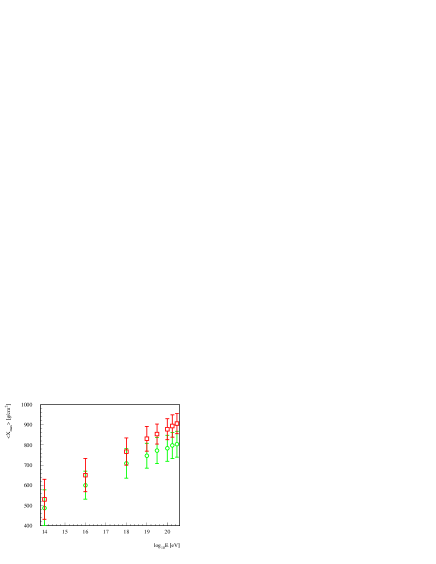
Figure 13: Simulation results for the average slant depth of maximum, $\langle X_{\rm max}\rangle$, for proton induced showers, plotted versus the logarithm of the primary energy. The error bars indicate the standard fluctuations (the RMS fluctuations of the means are always smaller than the symbols). The squares (circles) correspond to SIBYLL (QGSJET).

We have analyzed in detail the longitudinal development of the showers. The number of different kind of particles have been recorded as a function of the vertical depth for a number of different observing levels (more than 100).

The charged multiplicity, essentially electrons and positrons, is used to determine the number of particles and the location of the shower maximum by means of four-parameter fits to the Gaisser-Hillas function [31]. In Fig. 13, $\langle X_{\rm max}\rangle$ is plotted versus the logarithm of the primary energy for both, the SIBYLL and QGSJET cases. It shows up clearly that SIBYLL showers present higher values for the depth of the maximum, and that the differences between the SIBYLL and QGSJET cases increase with the primary energy. This is consistent with the fact that SIBYLL produces less secondaries than QGSJET –as discussed before– and as a result, there is a delay in the electromagnetic shower development which is strongly correlated with $\pi^{0}$ decays. The fluctuations, represented by the error bars, decrease monotonously as long as the energy increases, passing roughly from 95 g/cm² at $E=10^{14}$ eV to 70 g/cm² at $E=10^{20.5}$ eV.

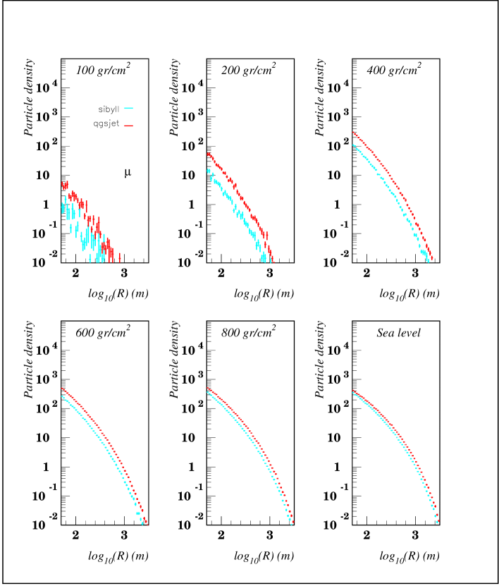
Figure 14: Comparison between the recorded muon lateral distributions displayed by SIBYLL and QGSJET at different atmospheric altitudes. Incident primary energy $10^{19}$ eV.

Using the recorded particle data, we have evaluated lateral distributions not only at ground altitude but also at predetermined observing levels. In the Figs. 14 and 15 we present the distributions corresponding to a subset of all the levels considered, taking into account particles whose distances to the shower axis are larger than 50 m.

The high-altitude lateral distributions show important differences between SIBYLL and QGSJET; such differences diminish as long as the shower front gets closer to the ground level. The behaviour can be explained taking into account the differences between the number of SIBYLL and QGSJET secondaries previously reported. Due to the fact that SIBYLL produces less number of secondaries, they have –in average– more energy and therefore the number of generations of particles undergoing hadronic collisions is increased with respect to the QGSJET case. As a result, during the shower development SIBYLL is called more times than QGSJET, and this generates a compensation that tends to reduce the difference in the final number of hadronic secondaries produced during the entire shower, and consequently in the final decay products, that is, electrons, gammas and muons.

The lateral distributions of electromagnetic particles are remarkably similar at both $\langle X_{\rm max}\rangle$ and ground level. However, it comes out from a more detailed analysis of the ground distributions that they are not strictly coincident and that the ratio between SIBYLL and QGSJET predictions does depend on $r$, the distance from the core. In fact, for electrons, this ratio runs from 1.25 for small $r$ to 0.73 for $r\sim 1000$ m, being equal to 1 at $r\sim 350$ m. A similar behaviour is observed for gammas where the lateral distributions intersect at $r\sim 1000$ m. In the case of lateral muon distributions, QGSJET predicts a higher density for all distances, but the SIBYLL/QGSJET ratio is not constant, ranging from 0.74 near the core to 0.56 at 1000 m.

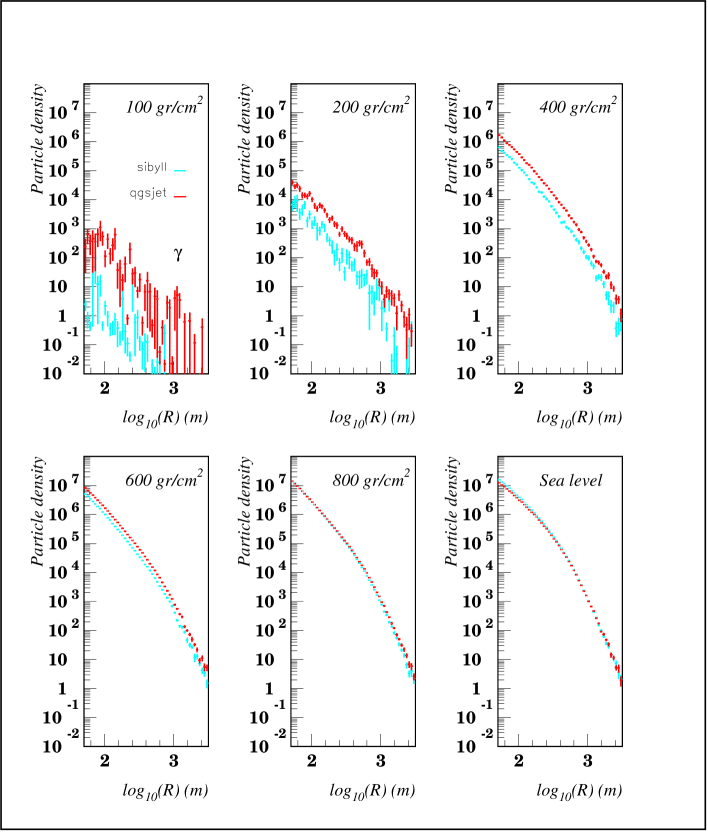
Figure 15: Same as Fig. 14 for the case of gammas.

Summing up, the most oustanding difference between SIBYLL and QGSJET is reflected in the predicted number of secondaries after single $p$-$\bar{p}$ and $\bar{p}$-nuclei collisions. Such a difference increase steeply with rising energy. The different number of secondaries predicted remains noticeable during the first stages of the shower development, however, the evolution of lateral distributions along the longitudinal shower path allows us to clearly observe how the differences in the distributions become monotonously damped, yielding rather similar shapes when reaching the ground. Further, we have shown that the differences observed at ground level do depend on the distance to the shower core. Consequently, we are convinced that it will be possible to obtain relevant information about the hadronic interactions in air showers from the measurement of particle densities at distances far from (as well as close to) the shower core. This can be achieved if CR experiments are designed with appropiate dynamic ranges.

Measurement of particle numbers at high atmospheric altitudes (fluorence detectors) together with shower maximun and changes rates, should contribute positively in the understanding of hadronic interactions if the kind of cosmic particle that induces the shower could be determined separately. Finally, it should be noted that most of the model discrepancies in hadronic interactions will be naturally reduced with the help of data obtained from future accelerator experiments like the well known Large Hadron Collider (LHC).

5 Looking Forward

Cosmic rays of extremely high energy are a weird phenomenon of nature for which no truly satisfactory explanation has been found yet. This may simply reflect our present ignorance of conditions or processes in some highly energetic regions of the Universe - or may imply that exotic mechanisms are at play.

After thirty years of careful work by several groups all over the world, we are in possession of a tantalizing body of data, sufficient to raise our curiosity and wonder, but not to succeed unravelling in the mistery. The coming avalanche of high quality CR-observations promises to make the begining of the next millenium an extremely exciting period for CR-physics.

References

- [1] V. F. Hess, Phys. Z. 13, 1804 (1912).
- [2] P. Auger et al., Comptes Rendus 206, 1721 (1938); P. Auger, Rev. Mod. Phys. 11, 288 (1939).
- [3] A. A. Penzias and R. W. Wilson, Ap. J 142,419 (1965).
- [4] K. Greisen, Phys. Rev. Lett. 16, 748 (1966); G. T. Zatsepin and V. A. Kuz’min, Pis’ma Zh. Éksp. Teor. Fiz. 4, 114 (1966) [JETP Lett. 4, 78 (1966)].
- [5] S. Yoshida and H. Dai, J. Phys. G 24, 905 (1998).
- [6] D. J. Bird et al., Phys. Rev. Lett. 71, 3401 (1993).
- [7] T. Stanev, P. L. Biermann, J. Lloyd-Evans, J. P.Rachen and A. A. Watson, Phys. Rev. Lett., 75, 3056 (1995).
- [8] N. Hayashida et al., Phys. Rev. Lett. 77, 1000 (1996).
- [9] D. J. Bird et al., astro-ph/9806096.
- [10] N. Hayashida et al., astro-ph/9807045.
- [11] M. Takeda et al., Phys. Rev. Lett. 81, 1163 (1998)
- [12] M. Hillas, Nature 395, 15 (1998).
- [13] G. R. Farrar and P. L. Biermann, Phys. Rev. Lett. 81, 3579 (1998).
- [14] R. J. Protheroe, talk presented at International School of Cosmic Ray Astrophysics: 10th Course: Toward the Millenium in Astrophysics: Problems and Prospects, Erice, Italy, 12-26 de junio 1996; astro-ph/9612212.
- [15] E. Waxman, Phys. Rev. Lett. 75, 386 (1995); M. Vietri, Ap. J. 453, 883 (1995); M. Milgrom and V. Usov, Ap. J. 449, L37 (1995).
- [16] T. Stanev, R. Schaefer and A. Watson, Astropart. Phys. 5, 75 (1996); A. Dar, astro-ph/9811196.
- [17] P. Bhattacharjee and G. Sigl, astro-ph/9811011.
- [18] T. W. Kephart and T. J. Weiler, Astropart. Phys. 4, 271 (1996); D. J. H. Chung, G. R. Farrar and E. W. Kolb, Phys. Rev. D 57, 4606 (1998).
- [19] L. Gonzalez-Mestres, 25th Int. Cosmic Ray Conf., Durban, South Africa, 1997, eds. M. S. Potgieter, B. C.Raubenheimer and D. J. van der Walt, Vol.VI, p.113; S. Coleman and S. L. Glashow, hep-ph/9808446.
- [20] M. S. Morris and K. S. Thorne, Am. J. Phys. 56, 395 (1988).
- [21] F. Halzen, R. A. Vazquez, T. Stanev and V. P. Vankov, Astropart. Phys. 3, 151 (1995).
- [22] F. W. Stecker, Phys. Rev. Lett. 80, 1816 (1998); L. N. Epele and E. Roulet, Phys. Rev. Lett. 81, 3295 (1998); F. W. Stecker, Phys. Rev. Lett. 81, 3296 (1998); F. W. Stecker and M. H. Salamon, Ap. J. (to be published), astro-ph/9808110.
- [23] L. N. Epele and E. Roulet, J. High. Energy Phys. 9810:009 (1998)
- [24] E. Roulet, Phys. Rev. D 47, 5247 (1993).
- [25] R. J. Protheroe, talk presented at International School of Cosmic Ray Astrophysics: 10th Course: Toward the Millenium in Astrophysics: Problems and Prospects, Erice, Italy, 12-26 de junio 1996; astro-ph/9612213.
- [26] J. W. Elbert and P. Sommers, Ap. J. 441, 151 (1995).
- [27] T. J. Weiler, preprint VAND-TH-97-8, hep-ph/9710431; D. Fargion, B. Mele and A. Salis, astro-ph/9710029.
- [28] E. Waxman, astro-ph/9804023.
- [29] N. N. Kalmykov, S. S. Ostapchenko and A. I. Pavlov, Nucl. Phys. B (Proc. Supp.) B52, 17 (1997); N. N. Kalmykov and S. S. Ostapchenko, Yad. Fiz. 56, 105 (1993) [Phys. At. Nucl. 56, 346 (1993)]; A. B. Kaidalov, K. A. Ter-Martirosyan and Yu. M. Shabel’skii, Yad. Fiz. 43, 1282 (1986) [Sov. J. Nucl. Phys. 43, 822 (1986)].
- [30] R. S. Fletcher, T. K. Gaisser, P. Lipari and T. Stanev, Phys. Rev. D 50, 5710 (1994).
- [31] S. J. Sciutto, AIRES: A System for Air Shower Simulations, Auger technical note GAP-98-032 (1998); electronically available from: http://www-td-auger.fnal.gov:82.
- [32] F. W. Stecker, Phys. Rev. Lett. 21, 1016 (1968); V. S. Berezinsky, Yad. Fiz. 11, 399 (1970).
- [33] H. P. Gush, M. Halpern and E. H. Wishnow, Phys. Rev. Lett. 65, 537 (1990).
- [34] G. Blumenthal, Phys. Rev. D 1, 1596 (1970).
- [35] J. P. Rachen and P. L. Biermann, Astron. Astrophys. 272, 161 (1993).
- [36] I. Golyak, Mod. Phys. Lett. A 7, 2401 (1992).
- [37] Particle Data Group, L. Montanet et al., Phys. Rev. D 50, 1173, 1335 (1994).
- [38] V. S. Berezinsky and S. I. Grigor’eva, Zh. Eksp. Teor. Fiz. 93, 812 (1987) [Sov. Phys. JETP 66, 457 (1987)]; Astron. Astrophys. 199, 1 (1988).
- [39] L. A. Anchordoqui, M. T. Dova, L. N. Epele and J. D. Swain, Nucl. Phys. B (Proc. Suppl.) 52B, 249 (1997); Phys. Rev. D 55, 7356 (1997).
- [40] F. A. Aharonian and J. W. Cronin, Phys. Rev D 50, 1892 (1994); J. W. Cronin, Nucl. Phys. B (Proc. Suppl.) 28B, 213 (1992).
- [41] S. Yoshida and M. Teshima, Prog. Theor. Phys. 89, 833 (1993).
- [42] F. W. Stecker, Phys. Rev D 180, 1264 (1969); V. S. Berezinsky and G. T. Zatsepin, Yad. Fiz. 13, 797 (1971) [Sov. J. Nucl. Phys. 13, 453 (1971)].
- [43] J. L. Puget, F. W. Stecker and J. H. Bredekamp, Ap. J. 205, 638 (1976).
- [44] L. A. Anchordoqui, M. T. Dova, L. N. Epele and J. D. Swain, 25th Int. Cosmic Ray Conf., Durban, South Africa, 1997, eds. M. S. Potgieter, B. C. Raubenheimer and D. J. van der Walt, Vol.VII, p.353.
- [45] E. Roulet, private comunication.
- [46] P. P. Kronberg, Rep. Prog. Phys. 57,325 (1994).
- [47] C. T. Hill and D. N. Schramm, Phys. Rev. D 31, 564 (1985).
- [48] F. W. Stecker, Nature 342, 401 (1989).
- [49] M. Abramowitz, I. A. Stegun, “Handbook of Mathematical Functions” (Dover, New York, 1970).
- [50] F. A. Aharonian, B. L. Kanevsky and V. V. Vardanian, Astrophys. Space Sci. 167, 93 (1990).
- [51] S. Lee, FERMILAB-Pub-96/066-A.
- [52] B. Binggeli, G. A. Tammann and A. Sandage, Astron. J. 94, 251 (1987).
- [53] M. T. Dova, L. Epele and C. Hojvat, 25th Int. Cosmic Ray Conf., Durban, South Africa, 1997, eds. M. S. Potgieter, B. C. Raubenheimer and D. J. van der Walt, Vol.VII, p.381.
- [54] M. T. Dova, L. N. Epele and C. Hojvat, work in progress.
- [55] L. A. Anchordoqui, M. T. Dova, L. N. Epele and J. D. Swain, Phys. Rev. D 57, 7103 (1998).
- [56] K. Meisenheimer, et al., Astron. Astrophys. 219, 63 (1989).
- [57] R. D. Blandford and M. J. Rees, Mon. Not. R. Astr. Soc. 169, 395 (1974). See also, K. S. Thorne, R. H. Price and D. A. Macdonald, Black Holes: The Membrane Paradigm (Yale University Press, 1986), chap.IV.
- [58] P. L. Biermann and P. A. Strittmatter, Ap. J. 322, 643 (1987).
- [59] T. A. Armstrong, et al., Phys. Rev. D 5, 1640 (1972).
- [60] A. R. Bell, Mon. Not. R. Astr. Soc. 182, 147 (1978); 182 443 (1978).
- [61] G. Cavallo, Astron. Astrophys. 269, 45 (1978).
- [62] J. O. Burns, E. D. Feigelson and E. J. Schreier, Ap. J. 273, 128 (1983).
- [63] N. Junkes et al., Astron. Astrophys. 269, 29 (1993).
- [64] C. G. T. Haslam, H. Stoffel, C. J. Salter and W. E. Wilson, Astron. Astrophys. S47, 1 (1982).
- [65] J. A. Combi and G. E. Romero, Astron. Astrophys. Suppl. 121, 11 (1997).
- [66] S. J. Tingay et al., (ASP Conference Series, eds. P. E. Hardee, A. H. Bridle and J. A. Zensus, 1996) Vol. 100, p.215.
- [67] L. Landau and E. Lifchitz, Fluid Mechanics (Pergamon Press, Oxford, 1958).
- [68] G. E. Romero, J. A. Combi, S. E. Perez Bergliaffa and L. A. Anchordoqui, Astropart. Phys. 5, 279 (1996). We take advantage here to note a typo error, Eq. (3) of [68] should read as Eq. (30).
- [69] A. G. Pacholczyk, Radio Astrophysics (Freeman, San Francisco, 1970).
- [70] J. E. Grindlay et al., Ap. J. 197, L9 (1975).
- [71] R. W. Clay, P. R. Gerhardy and D. F. Liebing, Aust. J. Phys. 37, 91 (1984).
- [72] N. E. B. Killeen, G. V. Bicknell and R. A. Ekers, Ap. J. 302, 306 (1986).
- [73] O. B. Slee, Aust. J. Phys. Suppl. 43, 1 (1997).
- [74] N. E. B. Killeen and G. V. Bicknell, Ap. J. 324, 198 (1988).
- [75] P. L. Biermann, Max-Plank-Institute für Radioastronomie, preprint No. 739.
- [76] L. A. Anchordoqui, G. E. Romero, S. E. Perez Bergliaffa and J. A. Combi, Mod. Phys. Lett. A 13, 3039 (1998).
- [77] J. W. Cronin, The Highest Energy Particles Produced in the Universe: Cosmic Rays, talk delivered at the Auger Project Workshop, Bariloche, Argentina, October 1995.
- [78] A. A. Watson, The Highest Energy Cosmic Rays: Recent Measurements and their Instrumentation, talk delivered at the Auger Project Workshop, Bariloche, Argentina, October 1995.
- [79] J. F. Ormes et al., 25th Int. Cosmic Ray Conf., Durban, South Africa, 1997, eds. M. S. Potgieter, B. C. Raubenheimer and D. J. van der Walt, Vol. V, p.273.
- [80] A. Capella, U. Sukhatme, C.-I. Tan & J. Tran Thanh Van, Phys. Rep. 236, 225 (1994).
- [81] A. B. Kaidalov, Phys. Lett B 116, 459 (1982); A. B. Kaidalov and K. A. Ter-Martirosyan, Phys. Lett. B 117, 247 (1982); Yad. Fiz. 39, 1545 (1984) [Sov. J. Nucl. Phys. 39, 979 (1984)].
- [82] K. Werner, Phys. Rep. 232, 87 (1993); C. A. García Canal Introduction a la physique des hadrons, (Série des cours et conférences sur la physique des hautes energies, N∘ 16, Centre de Recherches Nucléaires et Université Louis Pasteur, Strasbourg, France, 1980).
- [83] UA1 Collaboration, C. Albajar et al., Nucl. Phys. B 309, 405 (1988).
- [84] UA1 Collaboration, G. Arnison et al., Phys. Lett. B 118, 167 (1982).
- [85] T. K. Gaisser and T. Stanev, Phys. Lett. B 219, 375 (1989).
- [86] L. Durand & H. Pi, Phys. Rev. Lett. 58, 303 (1987).
- [87] R. J. Glauber, Nucl. Phys. B 21, 135 (1970).
- [88] G. M. Frichter, T. K. Gaisser and T. Stanev, Phys. Rev. D 56, 3135 (1997).
- [89] L. A. Anchordoqui, M. T. Dova, L. N. Epele and S. J. Sciutto, hep-ph/9810384.
- [90] Most of the electromagnetic algorithms are based on the well known MOCCA simulation program by A. M. Hillas, Nucl. Phys. B (Proc. Suppl.) 52, 29 (1997).
- [91] A. M. Hillas, in Proc. of the 16th International Cosmic Ray Conference, Tokyo, Japan, 1979 (University of Tokyo, Tokyo, 1979), Vol.8,p.7.; updated in, Proc. of the 17th International Cosmic Ray Conference, Paris, France, 1981 (CEN, Saclay, 1981), Vol.8,p.183.