A Simple Formulation of the Fast Multipole Method: Pseudo-Particle Multipole Method

Abstract

We present the pseudo-particle multipole method (P²M²), a new method to handle multipole expansion in fast multipole method and treecode. This method uses a small number of pseudo-particles to express multipole expansion. With this method, the implementation of FMM and treecode with high-order multipole terms is greatly simplified. We applied P²M² to treecode and combined it with special-purpose computer GRAPE. Extensive tests on the accuracy and calculation cost demonstrate that the new method is quite attractive.

1 Introduction

In this paper, we describe the pseudo-particle multipole method (P²M², Makino (1998)), a new method to express multipole expansion in fast multipole method(FMM, Greengard and Rokhlin (1987)) and treecode(Barnes and Hut (1986)). The basic idea of P²M² is to use a small number of pseudo-particles to express the multipole expansion. In other words, this method approximates the potential field of physical particles by the field generated by a small number of pseudo-particles. The distribution of pseudo-particles is determined so that it correctly describes the coefficients of multipole expansion.

P²M² offers two advantages over standard FMM which uses the multipole expansion directly. One advantage is its simplicity. As will be seen, the translation formulae used in P²M² are much simpler than their counterpart in standard FMM. Although the calculation cost is roughly the same for the same level of the accuracy, the simplicity implies that performance tuning and parallelization are easier.

Another advantage is that P²M²can take full advantage of special-purpose computers(GRAPE, Makino and Taiji (1998); Sugimoto et al. (1990)). GRAPE is a pipelined processor specialized to direct force calculation between particles. It offers the price-performance 100-1000 times better than that of general-purpose computers, for direct force calculation. Though treecode has been used on GRAPE(Athanassoula et al. (1998); Fukushige et al. (1991); Makino (1991)), it was difficult to go to high accuracy since only monopole can be calculated on GRAPE. With P²M² we can evaluate high-order terms using GRAPE, since these terms are expressed by distribution of pseudo-particles.

This paper is organized as follows. In section 2 we briefly describe the treecode and the FMM. In section 3 we give the description of Anderson’s method (Anderson (1992)), to which our method is closely related. In section 4 we describe the mathematics of P²M². In section 5 we present the result of numerical tests on the accuracy and the calculation cost for our implementation of treecode with P²M². In section 6 we discuss the implementation of treecode with P²M² on GRAPE. In section 7 we compare P²M² with Anderson’s method. In section 8 we summarize this paper.

2 Treecode and FMM

Here we give brief description of treecode and FMM. The treecode is described in section 2.1 and the FMM is described in section 2.2.

2.1 Treecode

In treecode, the forces from a group of distant particles are approximated by multipole expansions. Hierarchical tree structure is used for grouping of the particles.

Here we summarize the calculation procedure following Hernquist (1987); Hernquist and Katz (1989). First we construct an oct-tree structure by hierarchical subdivision of the space. The division procedure starts from the root node(root cell) of the tree which corresponds to a cube covering the entire system. The procedure is repeated until all leaf cells contain only one or zero particles.

In the next step we calculate the multipole expansions for all non-leaf cells. The calculation begins from the parents of the leaf cells and continued to the root cells ascending the tree structure. For a cell whose children are all leaves, the multipole expansion at its center is directly calculated from the distribution of the particles(leaves) in it. The expansion of a higher level cell is calculated from the expansions of its children. For each child cell, the center of the expansion is shifted to the center of the parent(M2M shift). All shifted expansions are then summed up at the center of the parent cell. Note that in most of existing implementation of treecode only up to quadrupole term is retained, and the center of mass is used as the center of expansion.

Then we calculate the total force on each particle. Starting from the root cell, we recursively traverse the tree structure collecting the force from cells(Barnes and Hut (1986)). We examine whether the cell in question is well separated from the particle or not. If the cell is well separated, the multipole expansion of the cell is evaluated at the position of the particle and added to the total force on the particle. In the case of a leaf cell, the force from the particle in it is used instead of the multipole expansion. If the cell is not well separated, we descend the tree to resolve the current cell into child cells, an then recursively examine each child in the same way. The condition that a cell is well separated is expressed as $l/d<\theta$. Here $l$ is the side length of the cell, $d$ is the distance between the cell and the particle, and $\theta$ is the opening angle that controls the accuracy. Leaf cells are always considered to be well separated.

The calculation cost of treecode is $O(N\log N)$, since the particle sees larger cell as distance becomes larger.

Treecode is widely used in astrophysics, in particular where accuracy requirement is modest. Most of existing implementations of treecode use only up to quadrupole moment and calculation cost rises quickly when high accuracy is required. The implementation detail is given in Hernquist (1987); Hernquist and Katz (1989). For the implementation on distributed-memory parallel computers, see Salmon et al. (1994).

2.2 FMM

Figure 1 shows the conceptual difference between treecode and FMM. In treecode, the forces from a cell to different particles are evaluated independently. In FMM, on the other hand, to calculate forces from cell $A$ to particles in cell $B$, we first calculate the spherical harmonics expansion(local expansion) of the potential field at the center of cell $B$ and then evaluate that expansion at the position of particles in cell $B$.

FMM was first presented in Greengard and Rokhlin (1987) for two dimensional case and was extended to three dimension in Greengard and Rokhlin (1988). The implementation detail for the three dimensional case is given in Board et al. (1994); Greengard and Rokhlin (1988); Hu et al. (1996); Pfalzner and Gibbon (1996); Schmidt and Lee (1991).

Figure 1: Approximation used in treecode(left) and FMM(right).

In the following we describe the non-adaptive version of FMM for three dimensional case. First we construct an oct-tree structure by hierarchical subdivision of the space. The division procedure starts from the root cell at refinement level $R=0$, which covers the entire system. Here we define the refinement level $R$ as the depth of the tree. We repeat the procedure until a given refinement level $R_{\rm max}$ is reached. The level $R_{\rm max}$ is chosen so that the average number of particles in one leaf cell roughly equals the prescribed number which is determined to optimize the calculation speed.

In the next step, we calculate the multipole expansions for all cells. This part is the same as that for treecode described in section 2.1.

Then, for each cell, we calculate the local expansion due to its interaction cells. Figure 2 shows the relation between a cell and its interaction cells. Interaction cells of a cell are defined as the children of its parent’s neighbor cells which are not its own neighbors. Here, neighbor cells are the cells at the same level which are in contact with the cell. The contribution from the interaction cells are calculated by converting their multipole expansion to the local expansions at the center of the objective cell(M2L conversion), and then summing them up.

In the next step, we add up the local expansions at different levels to obtain the total potential field at the leaf cells. We start calculation at $R=3$. For all cells in $R=3$, we shift the center of the local expansion of its parent(L2L shift), and then add it to the local expansion of the cell. By this procedure, all cells in $R=3$ will have the local expansion of the total potential field except for the contribution of the neighbor cells. By repeating this procedure for all levels, we obtain the potential field for all leaf cells.

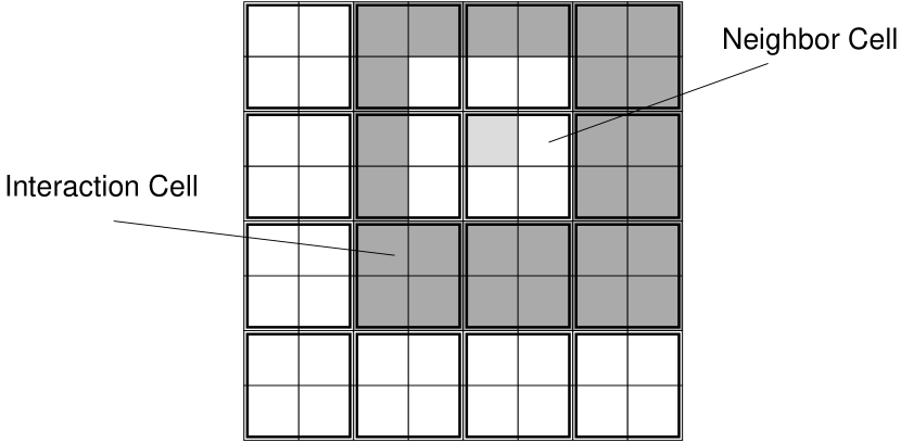
Figure 2: Relation between interaction cells(shaded) and neighbor cells of a hatched cell.

Finally, we calculate the total force on each particle. The total force is calculated as a sum of the distant and the neighbor contributions. The distant part is calculated by evaluating the local expansion of the leaf cell at the position of the particle. The neighbor part is directly calculated by evaluating the particle-particle forces.

In the following, we summarize the mathematics used in FMM. FMM requires two types of expansion of the potential and three transformations of them. One of the two expansions is the multipole expansion and the other is the local expansion. The multipole expansion of the potential $\Phi({\mbox{\boldmath{${r}$}}})$ up to $p$-th order is expressed as

$$\Phi({\mbox{\boldmath{${r}$}}})=\sum_{l=0}^{p}\sum_{m=-l}^{m=l}\frac{\alpha_{l}^{m}}{r^{l+1}}Y_{l}^{m}(\theta,\phi)$$ (1)

in spherical coordinates ${\mbox{\boldmath{${r}$}}}(r,\theta,\phi)$. Here $Y_{l}^{m}(\theta,\phi)$ is the spherical harmonics and $\alpha_{l}^{m}$ are the expansion coefficients. In order to approximate the potential field due to the distribution of particles, the coefficients should satisfy

$$\alpha_{l}^{m}=\frac{4\pi}{2l+1}\sum_{i=1}^{N}m_{i}r_{i}^{l}Y_{l}^{m*}(\theta_{i},\phi_{i}),$$ (2)

where $N$ is the number of particles to be approximated, $m_{i}$ and $(r_{i},\theta_{i},\phi_{i})$ are the masses and positions of the particles, and * denotes the complex conjugate. The local expansion $\Psi({\mbox{\boldmath{${r}$}}})$ up to $p$-th order is given by

$$\Psi({\mbox{\boldmath{${r}$}}})=4\pi\sum_{l=0}^{p}\sum_{m=-l}^{m=l}\beta_{l}^{m}r^{l}Y_{l}^{m}(\theta,\phi),$$ (3)

where $\beta_{l}^{m}$ is the expansion coefficients.

The three transformation required for FMM are the M2M shift, the M2L conversion, and the L2L shift. These transformation are expressed as follows:

$$\alpha_{l^{\prime}}^{m^{\prime}} = \sum_{l=0}^{p}\sum_{m=-l}^{m=l}T^{MM}_{l^{\prime}m^{\prime},lm}\alpha_{l}^{m}\hskip 30.0pt{\rm:M2M},$$ (4)

$$\beta_{l^{\prime}}^{m^{\prime}} = \sum_{l=0}^{p}\sum_{m=-l}^{m=l}T^{LM}_{l^{\prime}m^{\prime},lm}\alpha_{l}^{m}\hskip 30.0pt{\rm:M2L},$$ (5)

$$\beta_{l^{\prime}}^{m^{\prime}} = \sum_{l=0}^{p}\sum_{m=-l}^{m=l}T^{LL}_{l^{\prime}m^{\prime},lm}\beta_{l}^{m}\hskip 30.0pt{\rm:L2L}.$$ (6)

Using

$$a_{lm}=(-1)^{l+m}\frac{(2l+1)^{1/2}}{[4\pi(l+m)!(l-m)!]^{1/2}},$$ (7)

the transformation matrices are expressed as

$$T^{MM}_{l^{\prime}m^{\prime},lm} = 4\pi\frac{(-r_{t})^{l^{\prime}-1}Y^{(m^{\prime}-m)*}_{l^{\prime}-l}(\theta_{t},\phi_{t})a_{l^{\prime}-l,m^{\prime}-m}a_{lm}(2l^{\prime}+1)}{(2l+1)[2(l^{\prime}-l)+1]a_{l^{\prime}m^{\prime}}},$$ (8)

$$T^{LM}_{l^{\prime}m^{\prime},lm} = 4\pi\frac{(-1)^{l+m}Y^{(m^{\prime}-m)*}_{l^{\prime}+l}(\theta_{t},\phi_{t})a_{lm}a_{l^{\prime}m^{\prime}}}{r_{t}^{l^{\prime}+l+1}(2l+1)(2l^{\prime}+1)a_{l^{\prime}+l,m^{\prime}-m}},$$ (9)

$$T^{LL}_{l^{\prime}m^{\prime},lm} = 4\pi\frac{r_{t}^{l-l^{\prime}}Y^{(m-m^{\prime})*}_{l-l^{\prime}}(\theta_{t},\phi_{t})a_{l^{\prime}m^{\prime}}a_{l-l^{\prime},m-m^{\prime}}}{a_{lm}(2l^{\prime}+1)[2(l-l^{\prime})+1]}.$$ (10)

Here, $(r_{t},\theta_{t},\phi_{t})$ is the position of the new origin relative to the old one.

The calculation cost of FMM is $O(N)$. Therefore the scaling of FMM is better than that of treecode. However, at least in three dimension, comparisons indicate that treecode is faster for realistic number of particles (Blackston and Suel (1997)).

3 Anderson’s Method

Anderson (Anderson (1992)) proposed a simple formulation of FMM based on Poisson’s formula. Poisson’s formula gives the solution of the boundary value problem of the Laplace equation. When potential on the surface of a sphere of radius $a$ is given, the potential $\Phi$ at position ${r}$ is expressed as

$$\Phi({\mbox{\boldmath{${r}$}}})=\frac{1}{4\pi}\int_{S}\sum_{n=0}^{\infty}(2n+1)\left(\frac{a}{r}\right)^{n+1}P_{n}\left(\frac{{\mbox{\boldmath{${s}$}}}\cdot{\mbox{\boldmath{${r}$}}}}{r}\right)\Phi(a{\mbox{\boldmath{${s}$}}})ds$$ (11)

for $r>a$, and

$$\Phi({\mbox{\boldmath{${r}$}}})=\frac{1}{4\pi}\int_{S}\sum_{n=0}^{\infty}(2n+1)\left(\frac{r}{a}\right)^{n}P_{n}\left(\frac{{\mbox{\boldmath{${s}$}}}\cdot{\mbox{\boldmath{${r}$}}}}{r}\right)\Phi(a{\mbox{\boldmath{${s}$}}})ds$$ (12)

for $r<a$. Here $\Phi(a{\mbox{\boldmath{${s}$}}})$ is the given potential on the sphere surface. The range $S$ of the integration covers the surface of a unit sphere centered at the origin. The function $P_{n}$ denotes the $n$-th Legendre polynomial.

In Anderson’s method the value of $\Phi(a{\mbox{\boldmath{${s}$}}})$ is used to express the multipole/local expansion, while the original FMM uses the coefficients of the expansion terms. The advantage of Anderson’s method over the original FMM is its simplicity. The translation operators described in section 2.2 are all realized by evaluating the potential on points of the target sphere due to the source sphere. All such evaluations are performed using equation(11) and (12). These are by far simpler to implement the original FMM using equation(4)-(10).

In order to evaluate the integral in equation(11) and (12) numerically, we need to sample the values of $\Phi(a{\mbox{\boldmath{${s}$}}})$ on the surface of the sphere. The number of sample points required and the optimal positions of such points are given in Hardin and Sloane (1996).

4 Pseudo-Particle Multipole Method

P²M² is quite similar to Anderson’s method. The difference is that in P²M² we use the mass distribution on the surface of a sphere instead of the potential. The continuous mass distribution is again approximated by finite number of pseudo-particles, and the potential exerted by these pseudo-particles are calculated in the same way as that exerted by physical particles.

Conceptually, physical particles are converted to pseudo-particles in the following two steps. First we calculate multipole expansion. Then we assign mass to pseudo-particles so that they have the same multipole expansion as physical particles.

Calculation procedure of these two steps are as follows: In the first step we expand the potential with spherical harmonics. As we have seen in section 2.2, the multipole expansion and its coefficients are given by equation(1) and (2). In the second step we find a continuous mass distribution $\rho(a,\theta,\phi)$ on a sphere of radius $a$, which approximate the potential field. Then we approximate that distribution by pseudo-particles. The mass distribution should satisfy

$$\alpha_{l}^{m}=\frac{4\pi a^{l+2}}{2l+1}\int_{S}\rho(a,\theta,\phi)Y_{l}^{m*}(\theta,\phi)ds,$$ (13)

for $0\leq l\leq p$. Here $p$ is the highest order of multipole expansion to express and $S$ denotes the surface of the unit sphere. Because the spherical harmonics comprise an orthonormal system, $\rho(a,\theta,\phi)$ is expressed as

$$\rho(a,\theta,\phi)=\sum_{l=0}^{p}\sum_{m=-l}^{l}\frac{2l+1}{4\pi a^{l+2}}\alpha_{l}^{m}Y_{l}^{m}(\theta,\phi).$$ (14)

Following Hardin and Sloane (1996), we place $K$ points on the sphere so that they satisfy $\sum^{K}_{j=1}f({\mbox{\boldmath{${r_{j}}$}}})/K=\int_{S}f(a{\mbox{\boldmath{${s}$}}})ds$, where $f$ is any polynomial of degree at most $[2p+1]$(order $[2p+1]$ is necessary to guarantee orthogonality of spherical harmonics of up to order $p$), and ${\mbox{\boldmath{${r}$}}}_{j}$ are the positions of the distributed points. Thus equation(14) is replaced by

$$m_{j}=\frac{4\pi}{K}\sum_{l=0}^{p}\sum_{m=-l}^{l}\frac{2l+1}{4\pi a^{l}}\alpha_{l}^{m}Y_{l}^{m}(\theta_{j},\phi_{j}).$$ (15)

where $m_{j}$ are the masses of pseudo-particles located at ${\mbox{\boldmath{${r}$}}}_{j}(a,\theta_{j},\phi_{j})$. In practice, the masses $m_{j}$ of pseudo-particles are calculated directly from the positions ${\mbox{\boldmath{${r}$}}}_{i}(r_{i},\theta_{i},\phi_{i})$ and masses $m_{i}$ of physical particles. Combining equation(2) and (15), $m_{j}$ is expressed as

$$m_{j}=\frac{4\pi}{K}\sum_{l=0}^{p}\sum_{m=-l}^{l}\sum_{i=1}^{N}m_{i}\left(\frac{r_{i}}{a}\right)^{l}Y_{l}^{m}(\theta_{j},\phi_{j})Y_{l}^{m*}(\theta_{i},\phi_{i}).$$ (16)

Applying the addition theorem of spherical harmonics to equation(16), we obtain:

$$m_{j}=\sum^{N}_{i=1}m_{i}\sum^{p}_{l=0}\frac{2l+1}{K}\left(\frac{r_{i}}{a}\right)^{l}P_{l}(\cos\gamma_{ij}),$$ (17)

where $\gamma_{ij}$ is the angle between ${\mbox{\boldmath{${r}$}}}_{i}$ and ${\mbox{\boldmath{${r}$}}}_{j}$.

5 Accuracy of the Force Calculated with P²M²

Here we present the result of numerical tests for our implementation of treecode with P²M². In section 5.1 we compare the accuracy of P²M² and the original FMM for single particle. In section 5.2 we present the relation between the accuracy and the calculation cost for our implementation of treecode with P²M².

5.1 Accuracy of the Force Exerted from One Particle

We measured the accuracy of the potential calculated with P²M² and the original multipole expansion. A point mass located at ${\mbox{\boldmath{${p}$}}}(1,0,0)$ in spherical coordinate is used as the source of the potential. In figure 3 the error of the potential evaluated at point ${\mbox{\boldmath{${q}$}}}(q,2\pi/3,0)$ is plotted as a function of $q$ for both P²M² and the original multipole expansion. We can see that their agreement is quite good.

Figure 3: The error of potential calculated with P²M²(solid) and original multipole expansion (dashed). The error of potential generated by one particle at p are plotted against the distance from the origin to the evaluation point q. The error $e$ is defined as the difference from the exact potential. From top to bottom, four curves are for $p=1$, $2$, $4$ and $8$, respectively. The sphere radius $a$ is 1.0.

5.2 Accuracy of the Total Force

We measured the accuracy of the force calculated by the treecode with P²M². We used 262144 equal-mass particles uniformly distributed in a sphere. We measured the relative error $e$ of the force averaged over all the particles, and the calculation cost $c$ for $p$ = 1, 2, and 4. The average error $e$ is defined as

$$e^{2}=\frac{1}{N}\sum^{N}_{i=1}\frac{|\hat{\mbox{\boldmath{${f}$}}}_{i}-{\mbox{\boldmath{${f}$}}}_{i}|}{|{\mbox{\boldmath{${f}$}}}_{i}|}^{2},$$ (18)

where $\hat{\mbox{\boldmath{${f}$}}}_{i}$ is the force calculated with treecode and ${\mbox{\boldmath{${f}$}}}_{i}$ is the force calculated with direct summation method. We define the cost $c$ as the average number of (pseudo)-particle-particle interactions evaluated for one particle. Figure 4 shows the results. We can see that P²M² version with high-order terms is faster than the original version with monopole term, when high accuracy ($e<10^{-4}$) is required.

Figure 4: The error $e$ plotted against the calculation cost $c$(top-left panel) and the opening angle $\theta$(top-right panel). The relation between $c$ and $\theta$ is also shown in the bottom-left panel. Thick and thin curves denote treecode with and without P²M², respectively. Solid, long dashed, and short dashed curves are for $p=1$, $2$, and $4$, respectively.

6 P²M² Treecode on GRAPE

We implemented the treecode with P²M² on GRAPE (Makino and Taiji (1998); Sugimoto et al. (1990)). GRAPE is a special-purpose computer for gravitational $N$-body problem(figure 5). It consists of general-purpose host and special-purpose backend which calculates particle-particle interaction.

Figure 5: The GRAPE system.

With P²M², high-order terms of multipole expansion are expressed as particles. Therefore we can implement FMM and treecode with arbitrary order of multipole expansion on GRAPE systems. Previously, we could use GRAPE only to evaluate monopole terms.

Figure 6 shows the timing results of our treecode. The CPU time per timestep is measured on DEC AlphaServer 8400 5/300 (DEC 21164, 300MHz, one processor) with and without GRAPE-4(Makino et al. (1997)). We used a uniform distribution of 262144 particles in a sphere. The calculation with GRAPE-4 is 10–100 times faster than that without GRAPE-4. The gain becomes larger as we increase $p$ or decrease $\theta$. Thus we can conclude that the combination of P²M² and GRAPE is quite attractive if high accuracy is required.

Figure 6: Performance of P²M² treecode with and without GRAPE-4. The CPU time per one timestep is plotted for the opening angle $\theta$(left panel) and the force calculation error $e$(right panel). Thick and thin curves are the results with and without GRAPE-4, respectively. Solid, long dashed, and short dashed curves are for $p=1$, $2$, and $4$, respectively.

7 Relation between P²M² and Anderson’s Method

P²M² and Anderson’s method are quite similar. Both approximate the multipole expansion by discrete values on points on a sphere. The difference is that P²M² assigns mass to points while Anderson’s method assigns potential.

P²M² has two advantages over Anderson’s method. One is that the calculation of M2L part is significantly simpler for P²M² since the expanded potential $\Phi$ is evaluated as the summation of the potential due to pseudo-particles. The expression of $\Phi$ in P²M² is given by

$$\Phi({\mbox{\boldmath{${r}$}}})=\sum_{j=1}^{K}\frac{m_{j}}{r},$$ (19)

while the expression for Anderson’s method is given by equation(11). Since M2L is dominant part in FMM calculation, total calculation speed for the same expansion order would be faster for P²M². As we have seen in section 6, P²M² has an additional advantage that it can make use of special-purpose computers to achieve further speed up.

The other advantage is that the accuracy of the force calculated with P²M² is higher than that with Anderson’s method for the same expansion order. In Anderson’s method, the potential due to particles are converted to the potential on the sphere surface. The potential evaluated during this conversion is expressed as $m_{i}/r$ and not truncated to the $p$-th order. Therefore “aliasing error” is introduced into the potential during this conversion. This error tends to degrade the accuracy. In P²M², this aliasing error is completely suppressed. Of course, it is easy to modify Anderson’s method to use the truncated form. Such a modification would significantly improve the overall accuracy.

8 Summary

In this paper, we present P²M², a new method to express multipole expansion used in FMM and treecode. In P²M², multipole expansion is expressed by pseudo-particles on a sphere. P²M² has two advantages over the original multipole expansion. One is its simplicity and the other is that it can effectively use special-purpose computers. We implemented treecode with P²M² and evaluated its performance with and without GRAPE-4. We found that GRAPE-4 accelerates the calculation by a factor of 10-100. We conclude that P²M² is a quite attractive method to implement FMM and treecode.

References

- Anderson (1992) C. R. Anderson, An implementation of the fast multipole method without multipoles, SIAM Journal on Scientific and Statistical Computing, 13 (1992), pp. 923–947.
- Athanassoula et al. (1998) E. Athanassoula, A. Bosma, J.-C. Lambert, and J. Makino, Performance and accuracy of a GRAPE-3 system for collisionless -body simulations, Monthly Notices of the Royal Astronomical Society, 293 (1998), pp. 369–380.
- Barnes and Hut (1986) J. E. Barnes and P. Hut, A hierarchical force calculation algorithm, Nature, 324 (1986), pp. 446–449.
- Blackston and Suel (1997) D. Blackston and T. Suel, Highly portable and efficient implementations of parallel adaptive N-body methods, Proceedings of SC97, ACM, 1997.
- Board et al. (1994) J. A. Board, Jr., Z. S. Hakura, W. D. Elliott, and W. T. Rankin, Scalable Variants of multipole-based algorithms for molecular dynamics applications, Proceedings of the Seventh SIAM Conference on Parallel Processing for Scientific Computing(edited by Bailey et al.), SIAM, Philadelphia, 1995, pp. 295–300.
- Fukushige et al. (1991) T. Fukushige, T. Ito, J. Makino, T. Ebisuzaki, D. Sugimoto, and M. Umemura, GRAPE-1A: Special-purpose computer for N-body simulation with a tree code, Publication of the Astronomical Society of Japan, 43 (1991), pp. 841–858.
- Greengard and Rokhlin (1988) L. Greengard and V. Rokhlin, Rapid evaluation of potential fields in three dimensions, Vortex Methods(edited by C. Anderson and C. Greengard), number 1360 in Lecture Notes in Mathematics (1988), Springer-Verlag, Berlin, pp. 121–141.
- Greengard and Rokhlin (1987) L. Greengard and V. A. Rokhlin, Fast algorithm for particle simulations, Journal of Computational Physics, 73 (1987), pp. 325–348.
- Hernquist (1987) L. Hernquist, Performance characteristics of tree codes, Astrophysical Journal Supplement, 64 (1987), pp. 715–734.
- Hernquist and Katz (1989) L. Hernquist and N. Katz, TREESPH — a unification of SPH with the hierarchical tree method, Astrophysical Journal Supplement, 70 (1989), pp. 419–446.
- Hardin and Sloane (1996) R. H. Hardin and N. J. Sloane, McLaren’s improved snub cube and other new spherical designs in three dimensions, Discrete and Computational Geometry, 15 (1996), pp. 429–441.
- Hu et al. (1996) Y. Hu, S. L. Jonsson, and S.-H. Teng, A data-parallel adaptive -body method, Proceedings of the Eighth SIAM Conference on Parallel Processing for Scientific Computing, SIAM, 1997, (CD-ROM).
- Makino (1991) J. Makino, Treecode with a special-purpose processor, Publication of the Astronomical Society of Japan, 43 (1991), pp. 621–638.
- Makino et al. (1997) J. Makino, M. Taiji, T. Ebisuzaki, and D. Sugimoto, GRAPE-4: a massively parallel special-purpose computer for collisional -body simulations, Astrophysical Journal, 480 (1997), pp. 432–446.
- Makino (1998) J. Makino, Yet another fast multipole method without multipoles — pseudo-particle multipole method, submitted to Journal of Computational Physics, astro-ph/9806213.
- Makino and Taiji (1998) J. Makino and M. Taiji, Special purpose computer for scientific simulations — the GRAPE systems, John Wiley and Sons, Chichester, 1998.
- Pfalzner and Gibbon (1996) S. Pfalzner and P. Gibbon, Many-body tree methods in physics, Cambridge University Press, New York, 1996.
- Salmon et al. (1994) J. K. Salmon, G. S. Winckelmans, and M. S. Warren, Fast parallel treecodes for gravitational and fluid dynamical -body problems, International Journal of Supercomputer Applications, 8 (1994), pp. 129–143.
- Schmidt and Lee (1991) K. E. Schmidt and M. A. Lee, Implementing the fast multipole method in three dimensions, Journal of Statistical Physics, 63 (1991), pp. 1223–1235.
- Sugimoto et al. (1990) D. Sugimoto, Y. Chikada, J. Makino, T. Ito, T. Ebisuzaki, and M. Umemura, A special-purpose computer for gravitational many-body problems, Nature, 345 (1990), pp. 33–35.