STIS Observations of He II Gunn-Peterson Absorption
Toward Q 0302–003 ^†

Abstract

The ultraviolet spectrum (1145–1720 Å) of the distant quasar Q 0302–003 ($z=3.286$) was observed at 1.8 Å  resolution with the Space Telescope Imaging Spectrograph aboard the Hubble Space Telescope. A total integration time of 23,280 s was obtained. The spectrum clearly delineates the Gunn-Peterson He II absorption trough, produced by He II Ly$\alpha$  along the line of sight over the redshift range $z=2.78-3.28$. Its interpretation was facilitated by modeling based on Keck HIRES spectra of the H I Ly$\alpha$  forest (provided by A. Songaila and by M. Rauch and W. Sargent). We find that near the quasar, He II Ly$\alpha$  absorption is produced by discrete clouds, with no significant diffuse gas; this is attributed to a He II “proximity effect” in which the quasar fully ionizes He in the diffuse intergalactic medium, but not the He in denser clouds. By two different methods we calculate that the average He II Ly$\alpha$  opacity at $z\approx 3.15$ is $\tau\geq 4.8$. In the Dobrzycki-Bechtold void in the H I Ly$\alpha$  forest near $z=3.18$, the average He II opacity $\tau=4.47^{+0.48}_{-0.33}$. Such large opacities require the presence of a diffuse gas component as well as a soft UV background spectrum, whose softness parameter, defined as the ratio of the photo-ionization rate in H I over the one in He II $S\equiv\Gamma^{\mathrm{J}}_{\mathrm{H}I}/\Gamma^{\mathrm{J}}_{\mathrm{H}eII}\simeq 800$, indicating a significant stellar contribution. At $z=3.05$, there is a distinct region of high He II Ly$\alpha$  transmission which most likely arises in a region where helium is doubly ionized by a discrete local source, quite possibly an AGN. At redshifts $z<2.87$, the He II Ly$\alpha$  opacity detected by STIS, $\tau=1.88$, is significantly lower than at $z>3$. Such a reduction in opacity is consistent with Songaila’s (1998) report that the hardness of the UV background spectrum increases rapidly from $z=3$ to $z=2.9$.

${}^{\phantom{1}1}$ Laboratory for Astronomy & Solar Physics, Code 681, NASA/GSFC, Greenbelt MD 20771, USA
${}^{\phantom{1}2}$ National Optical Astronomy Observatories, Tucson, AZ 85726, USA
${}^{\phantom{1}3}$ Princeton University Observatory, Princeton, NJ 08544, USA
${}^{\phantom{1}4}$ Queen’s College, Oxford OX1 4AW, England
${}^{\phantom{1}5}$ heap@srh.gsfc.nasa.gov
${}^{\phantom{1}6}$ williger@tejut.gsfc.nasa.gov
${}^{\phantom{1}7}$ asmette@band3.gsfc.nasa.gov
${}^{\phantom{1}8}$ hubeny@tlusty.gsfc.nasa.gov
${}^{\phantom{1}9}$ msahu@panke.gsfc.nasa.gov
¹⁰ ebj@astro.princeton.edu
¹¹ tripp@astro.princeton.edu
¹² jonathan.winkler@queens.oxford.ac.uk

$\dagger$Based on observations with the NASA/ESA Hubble Space Telescope, obtained at the Space Telescope Science Institute, which is operated by the Association of Universities for Research in Astronomy, Inc., under NASA contract NAS5-26555.

1 INTRODUCTION

Once-ionized helium is the most abundant absorbing ion in the intergalactic medium (IGM). It outnumbers H I by a factor equal to the ratio of the ion number densities $n_{\mathrm{H}eII}/n_{\mathrm{H}I}\gtrsim 100$, and therefore serves as an ideal tracer of the IGM in the early universe ($z>2$). The presence of He II is signaled by absorption of He II Ly$\alpha$  $\lambda 304$ Å  redshifted to the far-ultraviolet (far-UV) where it can be observed by space observatories such as HST. If He II ions reside in clumps or clouds positioned along the line of sight to a quasar, they produce discrete absorption lines similar to the H I Ly$\alpha$ forest. But if instead they are diffused throughout the IGM, they will smoothly depress the flux level of a quasar shortward of its He II Ly $\alpha$ emission line. This is known as the Gunn-Peterson effect ([18]; [45]). Although the Gunn-Peterson opacity was originally formulated for H I, there is an analogous formula for He II:

$$\tau_{\mathrm{HeII}}(z)=\frac{c}{H_{\mathrm{o}}}~{}\frac{n_{\mathrm{HeII}}(z)~{}\sigma_{\mathrm{HeII}}}{(1+z)\sqrt{1+\Omega_{\mathrm{o}}z}}~{},$$ (1)

where $\sigma_{\mathrm{H}eII}\equiv(\pi e^{2}/m_{e}c^{2})f\lambda$ is the resonant scattering Ly$\alpha$  cross-section, and $f$ and $\lambda$ are the oscillator strength and wavelength of the He II Ly$\alpha$ line, respectively. The cross-section for H I is a factor of 4 larger than for He II. Hence, the ratio of opacities, $R=\tau_{\mathrm{HeII}}(z)/\tau_{\mathrm{HI}}(z)=\eta/4$, where $\eta\equiv N_{\mathrm{H}eII}/N_{\mathrm{H}I}$, and $N_{\mathrm{H}I}$ and $N_{\mathrm{H}eII}$ are the column densities of H I and He II, respectively. In evaluating the Gunn-Peterson optical depth and throughout this paper, we assume $H_{\mathrm{o}}=65~{}{\mathrm{\mbox{{\rm km~{}s}${}^{-1}$}}}~{}{\mathrm{M}pc}^{-1}$, $\Omega_{\mathrm{o}}=0.2$ and $\Lambda=0$.

He II Gunn-Peterson absorption has been explored in a variety of numerical simulations (e.g. [58]; [39]; [8]; [57]; [40], hereafter MHR). It has also been observed in four lines of sight. He II Gunn-Peterson absorption was first detected in the spectrum of the $z=3.286$ quasar, Q 0302–003, obtained with the Faint Object Camera (Jakobsen et al. 1994). However, because of the low spectral resolution and signal-to-noise ratio, the FOC data could not distinguish whether the absorption is produced by a uniformly distributed medium or by the He II counterpart of a forest of Ly$\alpha$  lines (cf. Songaila et al. 1995). Subsequent spectra covering the wavelength range, 1140–1530 Å  taken by the Goddard High Resolution Spectrograph (Hogan et al. 1997) confirmed the strongly depressed flux level shortward of He II Ly$\alpha$ in the QSO rest frame. It also showed a ledge in the flux level between 1280 – 1295 Å, attributed to the proximity effect ([3]; [58]; [17]), an effect of increased ionization of gas in the vicinity of the QSO. In the region from 1240 to 1280 Å, the GHRS spectrum was consistent with a null flux – however one with unacceptably large uncertainties (cf. Heap 1997).

Measurements of the He II Gunn-Peterson effect provide a test of cosmological models. Cosmological simulations can make concrete predictions of the epoch of IGM re-ionization from singly to doubly ionized helium (e.g. MHR), the timescale for the ionization change, and the characteristics of transition regions which might produce patchy He II absorption ([43]). Combining observations and simulations would constrain the density and ionization state of the gas, and the diffuse far-UV background radiation at $z\sim 3$.

In this paper, we present new observations of Q 0302–003 made with the Space Telescope Imaging Spectrograph (STIS). STIS brings several improvements over GHRS for faint, point-source spectroscopy: first, a lower instrumental background resulting in higher S/N ratios; second, an imaging format that allows direct measurement of the (sky + instrumental) background; and finally, a wider spectral range covered in a single exposure, presenting an opportunity to study the properties of the IGM over a broader range in redshift. The STIS observations presented here permit the strictest constraint to date for He II Gunn-Peterson absorption, over a wide spectral interval, and thus offer a significant advance in our understanding of the physical processes at $z\sim 3$. In §2 and §3, we describe the new observations. We then analyze in detail three important aspects of Gunn-Peterson absorption: the opacity of the absorption trough (§4), the “proximity effect” (§5), and the appearance of opacity gaps in an otherwise solid wall of absorption (§6). In §7, we summarize the implications of our findings.

2 OBSERVATIONS AND REDUCTIONS

Our analysis of He II Gunn-Peterson absorption along the line of sight to Q 0302–003 relies on two sets of observations: a far-UV spectrum of the QSO taken with STIS at low resolution, and high-resolution Keck spectra obtained by Songaila and by Rauch and Sargent, which were kindly made available to us. In this section, we describe the two datasets and our techniques of data reduction.

2.1 STIS UV Spectra

We obtained STIS observations of Q 0302–003 in December 1997 during the course of two “visits,” each five orbits long (Program 7575). See Woodgate et al. (1998) and Kimble et al. (1998) for details of the instrument and its performance. The observation used the G140L grating which produces a spectrum covering the wavelength interval, 1145–1720 Å, at a nominal two-pixel resolution of 1.2 Å. The sensitivity decreases strongly with wavelength below its peak at 1300 Å: it is only 10% of its peak value at 1150 Å, less than 4% at 1145 Å, and zero at at 1140 Å. The total exposure time (10 orbits) was 23,280 s.

Because of the faintness of the QSO, we selected a rather wide entrance slit (0$\farcs$2) in order to maximize throughput. As a consequence, the resolution is degraded to about 3 pixels, or 1.8 Å. A wide slit also has the disadvantage of transmitting rather strong geo-coronal emission of H I Ly$\alpha$  and a triplet of O I centered at $\lambda 1302$ (cf. Figure 1). This can be a serious problem because Ly$\alpha$  lies in the Gunn-Peterson trough, and O I $\lambda 1302$ lies at its edge and might therefore interfere with the assessment of the “proximity effect”. To counteract this problem, we obtained the spectra in the “TIME-TAG” mode with the intention of using only those data recorded during the earth-shadow time. We found, however, that contamination by geo-coronal emission can be fully accounted for in the reduction. We therefore assembled all of the TIME-TAG data from each orbit into a conventional spectrogram.

Figure 1: STIS observations of Q 0302–003. The top panel shows a major portion of the co-added spectrogram (lines 310-970 on the detector format). The two bright emission lines are geo-coronal Lyman $\alpha$ (left) and OI $\lambda$1302 (right). The spectrum of the QSO has a strong continuum flux at $\lambda\gtrsim 1280$ Å, while the Gunn-Peterson absorption trough sets in at shorter wavelengths. Within this trough, there is a major flux finger at $\lambda$1231, and several minor regions of flux are visible shortward of Lyman $\alpha$. The dashed red lines delimit the regions used to determine the background in the STScI reduction (not used for this paper), while the solid red lines apply to the region we adopted. The bottom panel shows the extracted spectrum, including the gross spectrum (QSO + background) shown by the black line and the average of the background above and below the quasar (squiggly red line). In the reduction, the background was smoothed (smooth orange line). Since the STIS MAMA1 detector is a photon-counting imaging detector, the errors in the total counts are simply the square root of the counts.

The observations were reduced at the Goddard Space Flight Center with the STIS Investigation Definition Team (IDT) version of CALSTIS (Lindler 1998), which allowed us to make a customized treatment of the background. Such flexibility is needed in order to ensure accurate fluxes and opacities in the Gunn-Peterson trough. As shown in Figure 1, the background in a STIS G140L spectrogram is highly non-uniform. The strong geo-coronal emission at Ly$\alpha$ and O I $\lambda$1302 affects a region wider than the projected entrance slit because of grating scatter. An additional source of background is the bright, diffuse background at the short-wavelength region of the image (the MAMA1 “hotspot”; cf. Landsman 1998). The QSO spectrum intersects this hotspot roughly through the middle. Because of the non-uniformity of the background, we sampled the background in two zones on either side of the QSO spectrum as closely as possible to the QSO (30-pixel offset) using an extraction slit height 30 pixels high (red lines in Figure 1). In order to avoid smearing out the geo-coronal emission lines, we smoothed the background (15-point running mean, executed twice) only in the regions away from the emission lines. In contrast, the STScI data processing system (RSDP) samples the background of STIS G140L spectra within bands located $\pm 300$ pixels away from the QSO spectrum (inside each pair of dashed red lines in Figure 1) where the background is only half that of our measured background. The resulting spectrum shows a spurious residual flux in the Gunn-Peterson absorption trough.

Figure 2 shows our reduced spectrum overplotted with an error spectrum that assumes $\sqrt{N}$ statistics. Despite the low S/N ratio at short wavelengths, the residual flux below 1175 Å  is real, since we see repeated appearances of signals at about the $5\sigma$ level. There is also a feature just shortward of geocoronal Ly$\alpha$  detected at the $5\sigma$ level. The wavelength uncertainty is much harder to estimate. We made an on-board calibration between successive exposures, which ensures that the dispersion is precise. However, there is still the possibility of a shift in the spectral direction between the QSO spectrum and the spectrum of the calibration source. Such a shift might be induced by imperfect centering of the QSO within the 0$\farcs$2 slit (8 pixels wide) or by thermally-induced drifts between the QSO and calibration exposures. Indeed, we find a 3-pixel shift in the zeropoint of the wavelength scale between the first exposure in a visit and the other four. Because of these uncertainties, we allow for a $\pm$1 pixel (0$\farcs$025) offset in the observed wavelength scale. Consistency with the wavelength scale of the H I Lyman forest suggests that a 1.06-Å  shift (1.8 pixels) is in order.

Figure 2: The STIS spectrum of Q 0302–003 after applying a background correction. Top: the absolute flux distribution in erg s^-1 cm^-2 Å^-1 (solid line) showing He II absorption shortward of 1300 Å, overlaid with the 1 $\sigma$ uncertainty (dashed line). Bottom: a magnified portion of the spectrum in the Gunn-Peterson absorption trough. In this panel, the flux was normalized to unity at $F_{\mathrm{c}}=2.1\times 10^{-16}$ erg s^-1 cm^-2 Å^-1, and binned by 3 pixels in order to show the average flux in a resolution element.

The spectral resolution is also difficult to estimate because there are no sharp, well defined lines in the co-added spectrum. We therefore used the cross-dispersion profile of the co-added QSO spectrum as a proxy for the line spread function. The cross-dispersion profile grows broader toward shorter wavelengths. We estimate that in the Gunn-Peterson absorption trough, the FWHM is 3.1 pixels; thus the corresponding spectral resolution is 1.80 Å.

2.2 Keck HIRES Spectra

We used spectra of Q 0302–003 taken with the Keck HIRES spectrograph (Vogt et al. 1994) provided by A. Songaila and by M. Rauch and W. Sargent to compare H I Ly$\alpha$  absorption with the He II Ly$\alpha$  absorption in the STIS spectrum. Table 1 summarizes the data. Successive columns give the observed wavelength range of the echellogram in Å, the equivalent wavelength range applicable to the STIS spectrum (i.e. the observed wavelength divided by 4 for the He II /H I wavelength ratio), the observed resolution in km s^-1, the maximum signal-to-noise ratio, and observer/source of the data. Hu et al. (1995) and Rauch et al. (1999) provide reduction details for the Songaila and Rauch datasets respectively. We processed the Rauch data and estimated the 1$\sigma$ uncertainties from the detector noise and photon counting statistics; for the Songaila data we calculated the 1$\sigma$ uncertainties from the apparent rms noise in the spectrum itself. In our analysis, we relied on the Rauch spectrum at $\lambda\mathrel{\hbox to0.0pt{\lower 3.0pt\hbox{$\mathchar 536\relax$}\hss}\raise 2.0pt\hbox{$\mathchar 318\relax$}}4600$ Å  where it has higher S/N ratio; we used the Songaila spectrum at shorter wavelengths for some metal-line identifications and to improve our H I Ly$\alpha$ profile fits using higher members of H I Lyman series. We detected a 2–3% residual flux in the bottoms of saturated absorption lines in the Songaila data, but found that it makes no significant difference to our analysis.

Table 1: Keck HIRES Spectra of the H I Lyman Forest Toward Q 0302–003

$\lambda_{\mathrm{v}ac}$ (Å)	$\lambda/4$	$R$ (km/s)	$(S/N)_{\mathrm{max}}$	Observer
3650–5983	912-1496	8.3	170	Songaila
4220–6656	1050-1664	6.9	130	Rauch & Sargent

Absorption lines of H I, C IV and other ions detected in the Keck spectra were fitted with Voigt profiles with the program, VPFIT (Webb 1987). We base our redshifts on wavelengths corrected to the vacuum heliocentric frame. Higher members of the H I Lyman series were used wherever possible to constrain the profile fits. We estimate the completeness limit at $\log N_{\mathrm{H}I}\sim 13.0$ (cm^-2) based on the point at which the H I column density distribution turns over. Our results for redshift $z$, Doppler parameter $b_{\mathrm{H}I}$, and H I column density, $N_{\mathrm{H}I}$, largely agree with those published by Hu et al. (1995). The few differences that we find can be attributed to $(i)$ the higher resolution of the Rauch dataset, $(ii)$ newly identified metal lines, or $(iii)$ an accounting for the ink spot in the middle of the HIRES CCD. The absorption-line parameters for the H I systems will be used in §5 to model the He II absorption. A detailed line list will be presented elsewhere ([42]).

3 OBSERVATIONAL RESULTS

In this section, we present the STIS spectrum of Q 0302–003, which covers the wavelength interval, 267–402 Å  in the rest frame of the QSO. We make this presentation in the form of two comparisons. In §3.1, we compare the He II Ly$\alpha$  absorption trough ($\lambda_{\mathrm{r}est}<304$ Å) with the corresponding H I Ly$\alpha$  forest. In §3.2, we compare the He II Ly$\alpha$  absorption in the spectrum of Q 0302–003 with other lines of sight.

3.1 Comparison of the He II and H I Ly$\alpha$  Spectra

In order to measure the strength of He II Ly$\alpha$  absorption, it is necessary first to define the continuum flux distribution of the QSO in this spectral region. Of course, the continuum is not a directly observable quantity, since it has been blocked by He II Ly$\alpha$ absorption. We must therefore extrapolate the flux longward of the Gunn-Peterson trough. But even this continuum is contaminated by absorption by intervening systems. Figure 3 shows a “widened spectrum” of the QSO in order to highlight the absorption features longward of the Gunn-Peterson trough. (It was constructed by vertically shifting successive raw spectrograms by 2 pixels and superposing them.) There is a break in the spectrum at $\sim$1620 Å  suggestive of a Lyman limit system at $z=0.773$. We searched for its Mg II $\lambda 2800$ absorption but could not conclusively identify these metal lines, because they are obscured by strong H I lines. There is also a known metal-line system at $z=1.889$ (Hu et al. 1995). A strong absorption line ($W_{\lambda}=1.2$ Å) at 1689 Å  is probably He I Ly$\alpha$  $\lambda$584 from this system. Because of the absorption from these intervening systems, the QSO flux distribution is not a smooth power law and hence, not easily extrapolated to shorter wavelengths.

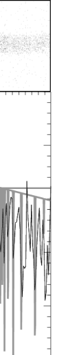
Figure 3: Far-UV flux distribution of Q 0302–003. Top: a 2-D display of the 10 spectra stacked vertically to show the reality of spectral features. Bottom: the observed flux distribution in units of erg s^-1 cm^-2 Å^-1. Two continuum estimates are shown as gray lines: one allowing for a Lyman limit system at $z=0.773$, and the other set to a constant value. The latter was used to normalize the flux in the Gunn-Peterson trough.

The lower panel of Figure 3 shows the observed flux distribution with two continuum estimates superposed. One attempts to account for the absorption of intervening systems via the program, CLOUDSPEC (Hubeny 1998), a combination of CLOUDY ([15]) and SYNSPEC (Hubeny et al. 1994). The other (and the one we adopt) is a flat continuum in wavelength (corresponding to $\alpha=2$, $f_{\nu}\sim\nu^{-\alpha}$) set at F_c=$2.1\times 10^{-16}~{}{\mathrm{e}rg}~{}{\mathrm{s}}^{-1}~{}{\mathrm{c}m}^{-2}~{}{\mathrm{\AA}}^{-1}$.

Figure 4 compares the STIS spectrum of Q 0302–003 with a simple model of the He II Ly$\alpha$  forest derived from the high-resolution (6 km s^-1) Keck/HIRES spectrum of the H I Ly$\alpha$  forest. The model calculation involved four steps: (i) estimate the optical depth in the H I Ly$\alpha$  lines from the flux of each data-point normalized to the apparent continuum, $\tau_{\mathrm{H}I}(\lambda)=-\ln(I_{\lambda}^{\mathrm{H}I})$; (ii) calculate the corresponding optical depth in the He II lines $\tau_{\mathrm{H}eII}(\lambda)$ at each data-point assuming a ratio of He II to H I optical depths $R=\tau_{\mathrm{H}eII}(\lambda)/\tau_{\mathrm{H}I}(\lambda)$; (iii) reconstitute the He II Ly$\alpha$  forest, $I(\lambda/4)=\exp(-\tau_{\mathrm{H}eII}(\lambda))$; and (iv) degrade the spectrum to the STIS resolution (1.8 Å). The values of $R=25$ and 100 used in the figure correspond to a ratio of He II to H I column densities, $\eta=N_{\mathrm{H}eII}/N_{\mathrm{H}I}=100$ and 400 respectively, and assume pure turbulent line broadening. The comparison makes clear what strong absorptions are part of the Ly$\alpha$  forest and what absorption is associated with the diffuse, or underdense, medium. For example, the high opacity of He II Ly$\alpha$  in the region, 1260-1280 Å, known as the Dobrzycki-Bechtold void ([11]; hereafter the D-B void), must originate in the diffuse medium. On the other hand, the H I opacity gap at 1231 Å  is also a gap in He II. At the very shortest wavelengths, there is a fair correlation of the observed spectrum with the simulated He II Ly$\alpha$  forest, suggesting that the opacity of the diffuse medium may be lower in this region. Close to the QSO redshift, there is also significant flux that has been interpreted as evidence of the proximity effect (Hogan et al. 1997).

Figure 4: Comparison of the observed (black line) and simulated (filled gray) spectra of Q 0302–003 in the Gunn-Peterson trough. The simulations assumed pure turbulent broadening ($\xi=1$) and two different values of the He II/H I optical depth ratio, R = 25 and 100. The region contaminated by geo-coronal Ly$\alpha$  was omitted in order to avoid confusion.

3.2 Comparison With Other Lines of Sight

To put the line of sight to Q 0302–003 in context, Figure 5 compares the STIS spectrum of Q 0302–003 with those of PKS 1935–692, a $z=3.18$ quasar observed by the GHRS (Tytler et al. 1995, Jakobsen 1996) and by STIS (Anderson et al. 1999), and HE 2347-4342, a $z=2.885$ QSO observed by GHRS (Reimers et al. 1997). (The raw observational data of PKS 1935–692 and HE 2347-4342 were re-reduced at Goddard.) The abscissa in this figure is now the redshift of He II Ly$\alpha$, $z=(\lambda/303.78)-1$, instead of observed wavelength. In each panel, the downward pointing arrow shows the wavelength of He II Ly$\alpha$  at the redshift of the QSO. Below, we discuss the three major features of the He II Ly$\alpha$  absorption trough: the proximity effect, the absorption trough itself, and gaps in the absorption.

Figure 5: Comparison of the He II Gunn-Peterson absorption trough plotted as a function of redshift for the He II line at 303.78 Å. Q 0302–003 and PKS 1935–692 were observed with STIS, and HE 2347-4342 by GHRS. The downward arrows denote the redshift of the QSO. As in Figure 4, the spectral region near geo-coronal Ly$\alpha$  is grayed out. In the case of PKS 1935–692, which has an intervening damped Ly$\alpha$  system at $z=0.30$, the predicted absorption spectrum from the DLA is also shown in gray as a warning that the opacity at $z<3$ should not be interpreted as Gunn-Peterson absorption.

The Proximity Effect. This term refers to an observed decrease in the number of H I Ly$\alpha$  - absorbing clouds in the neighborhood of a QSO, at least in part caused by the H-ionizing radiation field of the QSO. A He II proximity effect involving both He II-absorbing clouds and diffuse components of the IGM is also expected. It is best defined by the spectrum of Q 0302–003, although it is also evident in PKS 1935-692; however, note that the edge of the proximity zone is blocked by a pronounced gap in the absorption. In §5, we will use the observed flux distribution in the proximity zone to explore the shape of the radiation field of the QSO and the metagalactic background at $z\approx 3$.

The He II Gunn-Peterson Absorption Trough. Strong, continuous absorption is evident in all three quasar spectra outside of the proximity zone. Of the three, only the spectrum of Q 0302–003 has the broad baseline in redshift ($z=2.78-3.28$) needed for studying the evolution of the IGM. The spectrum of PKS 1935–692 would appear at first also to be useful for this purpose, but it is contaminated by a $z=0.30$, damped Ly$\alpha$  system ($\log N_{\mathrm{H}I}=21.2$) whose Lyman continuum absorption effectively blocks the light from the quasar corresponding to He II Ly$\alpha$ at $z<3.0$ (the shaded region in Figure 5). In §4, we will analyze the absorption trough in the spectrum of Q 0302–003 in detail.

Gaps in the Absorption Trough. At wavelengths shortward of the shelf of transmitted flux that we attribute to the proximity effect, there are significant gaps in an otherwise solid wall of absorption by He II. As can be seen in Figure 5, there are windows of transmitted flux in the spectrum of Q 0302–003 at $z=3.05$, PKS 1935–692 at $3.10$, and HE 2347–4342 at $z=2.87$ and $2.82$. Since these windows of transmitted flux are broader than our instrumental resolution and are not accompanied by similar, much narrower ones elsewhere, it is doubtful that they correspond to gaps appearing by chance among randomly distributed absorbing clouds. In §6, we shall argue that these coherent stretches of transmission are probably the result of discrete sources photo-ionizing the surrounding material.

Note how the morphology of low-opacity regions changes with redshift. At redshifts $z>3$ (and outside of the proximity zone), the opacity gaps are isolated, discrete, and major. In contrast, regions of transmission at $z\mathrel{\hbox to0.0pt{\lower 3.0pt\hbox{$\mathchar 536\relax$}\hss}\raise 2.0pt\hbox{$\mathchar 316\relax$}}2.9$ occur more frequently but with smaller amplitude. This changing morphology will be discussed in the following three sections.

4 THE He II GUNN-PETERSON ABSORPTION TROUGH

In this section, we make quantitative assessments of the He II Ly$\alpha$  optical depth of the IGM along the line of sight to Q 0302–003. These include both direct determinations of the average transmission within the He II Gunn-Peterson absorption trough (§4.1), and a more sensitive but less direct method that makes use of the low level of fluctuations in transmission in the trough (§4.2). Since the measurements cover a wide redshift range ($z=2.78-3.28$), we were able to trace the redshift evolution of the He II Ly$\alpha$  opacity. We find that it rises rapidly with redshift, a result that is compatible with a shift in the C IV/Si IV ratio between $z=2.9$ and $z=3.0$ reported by Songaila (1998) (§4.3). On the assumption that a lower He II Ly$\alpha$  opacity is due to a higher fraction of doubly-ionized helium, we follow the re-ionization history of helium over the redshift interval, $z=2.8-3.2$ (§4.4).

4.1 Measured Opacities

We estimated the He II Ly$\alpha$  opacity for different regions as shown in Figure 6. The upper panel shows the normalized flux (i.e. the relative transmission of the IGM) as a function of redshift, while the bottom panel shows the spectrum of apparent optical depths. The region labeled “D-B” is the Dobrzycki-Bechtold void (1991). Regions A and B are used together to characterize the He II opacity at $z\approx 3$ for comparison with theoretical predictions. The region labeled “S” corresponds to redshifts that Songaila (1998) identified as the high-ionization regime (cf. §4.3). We measured the average residual intensities in each region ($\bar{I}$) and converted them to representative optical depths ($\tau=-\ln\bar{I}$) with results listed in Table 2. Successive columns give the region ID, the number of data-points in the region, the average transmission and its uncertainty, the rms error of a single data-point, and the optical depth corresponding to the average of the transmitted intensities.

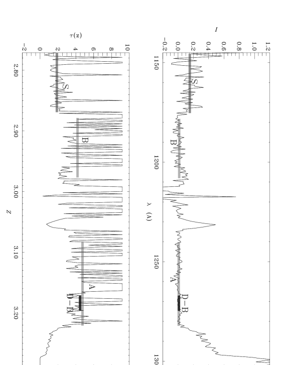
Figure 6: Transmissions (upper panel) and opacities (lower panel) in the Gunn-Peterson absorption trough. The selection of the different spectral regions is explained in the text. The measured values of the apparent transmissions and optical depths are given in Table 2 and depicted by gray bars.

Table 2: Measured Opacities in the Gunn-Peterson Trough

Region	$\bar{z}$	N	Ī	$\sigma$(I)	$\tau_{\mathrm{r}egion}$
D-B	3.18	14	0.0114 $\pm$ 0.0044	0.0164	$4.47^{+0.48}_{-0.33}$
A	3.15	73	0.0086 $\pm$ 0.0029	0.0246	$4.75^{+0.41}_{-0.29}$
B	2.93	52	0.0151 $\pm$ 0.0079	0.0567	$4.19^{+0.73}_{-0.42}$
S	2.82	52	0.1532 $\pm$ 0.0179	0.1292	$1.88^{+0.12}_{-0.11}$
A+B	3.06	125	0.0113 $\pm$ 0.0037	0.0410	$4.48^{+0.39}_{-0.28}$

In agreement with previous GHRS observations, the optical depth of the D-B void $\tau_{\mathrm{DB}}=4.47^{+0.48}_{-0.33}$ is quite high, implying that the absorption appears to be due to diffuse or underdense material. Alternatively, there may be a nearby starburst galaxy or other soft ionizing source that could ionize H I but not He II, thereby producing a low H I opacity but not affecting the He II opacity. As the GHRS spectrum only sampled the Gunn-Peterson trough above $z=3.1$, the measured opacities in the other regions (A, B, S) are new, and will be discussed later in this section.

The $rms$ errors quoted in the table give a measure of the random errors. There remains the question of systematic errors, which are the more serious of the two. Since the STIS detector is a pulse-counting detector with a linear response at low light levels, we can rule out the possibility that the low residual flux in the Gunn-Peterson trough is due to a systematic error in the response function. However, there could be a systematic error in the residual flux if the cross-dispersion (“vertical”) gradation in the background were not linear, so that the average of the upper and lower background regions would not be representative of the background under the QSO spectrum. We can put an upper limit on this systematic error by re-reducing the spectrograms with the upper background or lower background only. These alternate reductions produce residual fluxes in the Gunn-Peterson absorption trough that are well within the uncertainties quoted in the table. Other reduction procedures (15-point background smoothing applied twice, registration of the observations before co-addition) yield differences on the same order as adopting the upper or lower background only. We therefore interpret the errors listed in the table as representing total errors.

4.2 Opacity Fluctuations

Now that we have explicitly measured the opacities, we can obtain a more sensitive, but less direct result by looking for gaps in the opacity that appear by chance and comparing them with predictions. We find that a high opacity is required to produce the broad stretches of nearly zero transmission as seen, for example, in spectral region A. This region has 24 independent samples of width $\Delta z=0.0058$, where independent samples are assumed to be separated by the instrumental resolution (3 pixels). All 24 samples show a relative transmission, $\bar{I}\leq 0.030$ (cf. Figure 2), implying that the optical depths exceed $-\ln(0.03)=3.50$ everywhere in this region. We designate this opacity as $\tau_{\mathrm{l}imit}$. Even in the absence of extra ionizing sources, we should expect to see some variations caused by the random gaps in the overlapping of clouds. The fact that such variations do not cause observable transmission spikes implies that the average optical depth is greater than a certain amount – a value that we shall now evaluate.

Fardal, Giroux & Shull (1998) constructed a model for the clouds in the IGM based on the observed properties of the Ly$\alpha$ forest and then, on the basis of Monte Carlo simulations, found that fluctuations in the apparent opacity of He II, defined as $\tau\equiv-\ln\bar{I}$, over an interval $\Delta z$, follow the approximate relationship (their Eq. 17):

$$\left({\Delta\tau}\over\bar{\tau}\right)_{\mathrm{m}odel}\approx 0.03(\xi\,\eta_{100})^{-0.1}\Delta z^{-0.5}\left({1+z}\over 4\right)^{-1.0}~{},$$ (2)

where $\bar{\tau}$ is the average of $\tau$ over many intervals of $\Delta z$, and $\Delta\tau$ represents a deviation of $\tau$ from this average. The quantity $\xi$ is the characteristic ratio of the He II line width to that of H I (ranges from 0.5 to 1.0, depending on whether the line broadening is dominated by thermal or turbulent processes), and $\eta_{100}=N_{\mathrm{H}eII}/(100~{}N_{\mathrm{H}I})$.

Now consider the (very small) probability $p$ that a single sample of width $\Delta z$ shows a spike $\bar{I}\geq 0.030$, i.e. $\tau_{\mathrm{l}imit}\leq 3.50$. This quantity $p$ then represents the one-tail area below $\tau_{\mathrm{l}imit}$ for a normal distribution with a standard deviation $\Delta\tau$ centered on $\bar{\tau}$. The chances of not seeing a spike over all 24 samples is $e^{-24~{}p}$. We now determine the limiting condition that would create a 10% expectation of seeing no spikes in any of the samples, since this leads to a confidence level of 90% that we are not overestimating $\bar{\tau}$ and/or underestimating $\Delta\tau$. This happens when $p=-\ln(0.1)/24=0.096$ which is the one-tail area for $\sigma=1.30$ standard deviations below the center of the normal distribution. This requirement sets a lower limit for the average opacity,

$$\bar{\tau}>\tau_{\mathrm{l}imit}\left[1-\sigma\left({\Delta\tau\over\bar{\tau}}\right)_{\mathrm{m}odel}\right]^{-1}~{}.$$ (3)

For $\tau_{\mathrm{l}imit}=3.50$, $\sigma=1.30$, $\eta_{100}$ =3.5 (cf. §5.4.3), and $\xi=0.5$ or $1.0$, we obtain $\bar{\tau}>6.6$ and $6.2$, respectively. Both values are somewhat higher than the measured value, $\tau_{\mathrm{A}}=4.75\pm 0.4$ in Region A.

4.3 A Break in He II Ly$\alpha$ Opacity at $z=2.9-3.0$?

Songaila (1998) recently reported on a study of Keck HIRES spectra of 13 quasars, in which she found that the C IV/Si IV ratio at $z=2.9$ was 3.4 times higher than at $z=3.0$. Since the ionization potentials of Si IV (45.1 eV) and C IV (64.5 eV) straddle the ionization potential of He II (54.4 eV), C IV/Si IV serves as a proxy for the ionization state of helium, and she attributed the change in this ratio to a hardening of the metagalactic spectrum below $z=3.0$. However, Songaila’s findings were disputed by Boksenberg et al. (1998) who found no sudden change in ionization, although they did note a gradual increase in C IV/Si IV toward lower redshifts between $z\approx 3.8$ and $z\approx 2.2$.

The STIS spectrum of Q 0302–003 provides an opportunity to trace the ionization evolution of helium over a broad redshift range, $z=2.8-3.2$. (We assume that a lower He II opacity means a higher fraction of doubly ionized helium.) Our calculations with CLOUDY ([15]) indicate that the He III/He II ratio should change by at least as much as C IV/Si IV for a Madau et al. (1999) background radiation field at $z=3$. We therefore looked to see whether the He II opacities show a distinct change between $z=2.9$ and $z=3.0$. We find that Region S of Figure 6 does indeed show a residual flux in the Gunn-Peterson trough at $z<2.87$ implying an average transmission that corresponds to $\tau_{\mathrm{S}}=1.88$ in this region.

The redshift interval, $z=2.77-2.87$, however, is by no means a void in the conventional sense. Many H I Ly$\alpha$  forest lines occur there, in some cases with clear corresponding increases in He II opacity. To compare the $z<2.9$ and $z>3.0$ opacities, we selected those data points in Region S unassociated with features in the Lyman forest, i.e., positions identified as having a normalized H I transmitted flux greater than 0.95 even when degraded to STIS resolution. We find 10 non-contiguous data-points in Region S fulfilling this $I_{\mathrm{H}I}>0.95$ requirement. The He II opacity corresponding to the average transmission for these 10 data-points is $\tau=1.41\pm 0.06$, which is a factor of 3 times lower than in the D-B void. Similarly, the opacity for the whole Songaila region ($\bar{z}=2.82$) which includes numerous Ly$\alpha$  lines, $\tau_{\mathrm{S}}=1.88$, is a factor of 2.5 times lower than for Region A at $\bar{z}=3.15$. We conclude that the He II Gunn-Peterson data are in accord with Songaila’s assertion of an abrupt shift in ionization between $z=2.9$ and $z=3.0$.

4.4 Comparison with Cosmological Models

Observations of He II Ly$\alpha$  absorption give a direct connection with cosmological simulations if differences in resolution are taken into account. For example, simulations by Zhang et al. (1998) cover a cube only 9.6 comoving Mpc on a side with a cell size of 75 kpc³. In contrast, our STIS spectrum of the G-P trough covers a much larger distance (400 comoving Mpc) but at a coarser resolution ($\sim 2$ comoving Mpc), so it smooths over all of the fine-scale fluctuations predicted by theory. Nevertheless, we can apply the same kind of smoothing on the theoretical opacities by taking averages. Zhang et al. (1998, their figure 20) predict that the average He II opacity should increase from $\bar{\tau}=0.50$ at $z=2.4$, to $\bar{\tau}=0.83$ at $z=3$, and $\bar{\tau}=2.43$ at $z=4$.

The measurements listed in Table 2 imply that the total He II opacity rises more rapidly with redshift than the models (Zhang et al. 1998, Fardal et al. 1998). As shown in Figure 7, which combines data for HS 1700+6416 ([10]) with the measured opacities derived from Regions S, B, and A in the spectrum of Q 0302–003, the He II optical depth in Ly$\alpha$  increases sharply from $\tau=1.0$ at $z=2.4$ to $\tau\sim 4.7$ at $z=3.15$. The more sensitive estimates of the He II opacity based on the lack of opacity fluctuations suggest that it may rise with redshift even faster than shown. The top panel also plots the mean He II Ly$\alpha$ opacity predicted by Zhang et al.’s (1998) cosmological model. It shows that the model generally underestimates the He II Ly$\alpha$ opacity and does not reproduce the observed steep rise in opacity with increasing redshift.

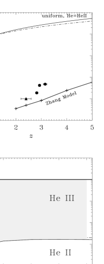
Figure 7: Evolution of the He II Ly$\alpha$  opacity (top) and helium ionization fractions (bottom). Top: The filled circles represent data from our STIS observations of Q 0302–003, while the filled triangle represents the HUT results for HS 1700+6416 (Davidsen et al. 1996). The bold curve shows the opacity predicted by Zhang et al. (1998). The other curves show the expected He II Ly$\alpha$  opacity if all helium were singly ionized and uniformly distributed. The assumed cosmological parameters are: $H_{\mathrm{o}}$=65 km s^-1Mpc^-1 and $\Omega_{\mathrm{o}}=0.2$, $\Lambda=0$ (solid line) , or $H_{\mathrm{o}}$=50 km s^-1Mpc^-1 and $\Omega_{\mathrm{o}}=1.0$, $\Lambda=0$ (dash-dot). Bottom: Implied helium ionization fractions in the redshift range observed by STIS, based on the assumption that all helium is once or doubly ionized. The fraction of HeII is only about 0.1 % at $z\sim 3$.

The top panel of Fig. 7 also shows the opacity expected if all helium were in the form of He⁺ and were uniformly distributed. Two curves are shown: one for our assumed cosmological parameters (solid line), the other for Madau et al.’s (1999), i.e. $H_{\mathrm{o}}$=50 km s^-1Mpc^-1, $\Omega_{\mathrm{o}}=1.0$ and $\Lambda=0$. In either case, the measured opacity is more than 600 times smaller than expected. The fact that we detect a small residual intensity in Regions A and B indicates that most, but not all, of the helium is doubly ionized at $z=3$. Accordingly, the bottom panel shows the implied fractions of He III and He II.

In summary, away from distinct gaps in the He II absorption, the Ly$\alpha$  opacity shows a sharp rise between $z=2.8$ and $z=3.2$. At $z\sim 3.15$, the optical depth is estimated at 4.7 or more. It therefore appears that we are witnessing the transition from a He II Ly$\alpha$  forest to a He II Gunn-Peterson trough. The sharp rise in opacity at $z\sim 3$ (interpreted as an increased fraction of He II ) is consistent with Songaila’s claim of a lower ionization level of the IGM at $z>3$ . However, we caution that these results are based on a single line of sight. Other lines of sight may give different results since He II is such a minor fraction of helium (0.16%). In fact, some of the large scatter in Songaila’s measured C IV/Si IV ratios may reflect such differences. We plan to pursue the question of a “universal epoch of reionization” by studies of the He II Gunn-Peterson effect along the sightlines to PKS 1935–692 and HE 2347–4342.

5 MODELS OF GUNN-PETERSON ABSORPTION AND THE PROXIMITY EFFECT

The He II opacities measured in §4 imply that the vast majority of He is doubly ionized at $z\sim 3$, presumably by the UV background. In this section, we derive the properties of the UV background at $z\sim 3$ from the H I and He II Ly$\alpha$  spectra of Q 0302–003. To pursue the matter, we constructed spectral models that take into account just one ionizing source, the QSO itself, in addition to the UV background. These models allow us (1) to identify regions within the proximity zone that are particularly sensitive to the shape of the UV background, and can thus be used to constrain it, and (2) to discriminate among the He II opacity gaps those likely caused by underdense regions in the IGM from those due to discrete ionizing sources. In the following sections, we describe the model input, calculations, and results.

5.1 Model Input

The three main inputs to the models are the observed flux distribution in the He II Gunn-Peterson absorption trough, the QSO flux distribution, and the physical parameters of the H I Ly$\alpha$  forest. Below, we describe our methods for estimating the QSO continuum flux distribution and the physical characteristics of the H I Ly$\alpha$  lines.

5.1.1 The spectral energy distribution of Q 0302–003

We estimated the ionizing flux distribution of the QSO from measurements of the apparent continuum combined with model continuum flux distributions. Figure 8 plots the theoretical luminosity distribution of Q 0302–003 along with observationally derived continuum points transformed to the quasar rest frame ($z=3.29$). The observed points are taken from our STIS data and from the ground-based spectrum obtained by Sargent, Steidel, & Boksenberg (1989). The STIS observations cover the restframe interval, 267 - 402 Å, or $7.5\times 10^{15}-1.12\times 10^{16}$ Hz. The SSB fluxes were multiplied by a factor of 1.25 to account for the depression of the apparent continuum by the multitude of lines that make up the Ly$\alpha$  forest. This factor was estimated from the normalized Songaila et al. spectrum (Table 1) degraded to the resolution of the spectrum obtained by Sargent et al. We found that a power law of the form $f^{\rm QSO}=f_{\mathrm{H}I}^{\mathrm{Q}SO}~{}(\nu/\nu_{\mathrm{H}I})^{-\alpha_{\mathrm{H}I}^{\rm QSO}}$ with ${\alpha_{\mathrm{H}I}^{\mathrm{Q}SO}}=1.9$, gives a good representation of the data from the optical to the far-UV ($\lambda_{\mathrm{r}est}=1000-304$ Å). In our models of the QSO flux distribution, we extrapolate this power law into the unobserved He II Lyman continuum as well.

Figure 8: Probable spectral energy distribution of Q 0302–003. The filled squares show the observed continuum flux transformed to the quasar rest frame. The upward-pointing arrows give the frequencies of HI Ly$\alpha$  (left) and the HI Lyman limit (right). The downward-pointing arrows show the same quantities for He II. The solid lines show two theoretical models of a bare accretion disc around a super-massive, Kerr black hole with a black-hole mass $M=2\times 10^{10}$ $M_{\odot}$ and the mass accretion rate $\dot{M}=24$ $M_{\odot}\,{\mathrm{y}r}^{-1}$ (upper curve); and $M=1.6\times 10^{10}$ $M_{\odot}$ and mass accretion rate $\dot{M}=16$ $M_{\odot}\,{\mathrm{y}r}^{-1}$ (lower curve). Both models assume an almost face-on disk, with inclination $\cos i=0.99$.

The two theoretical models shown in the figure are for a bare accretion disk around a super-massive, Kerr black hole, one with a black-hole mass $M=2\times 10^{10}$ $M_{\odot}$, and accretion rate $\dot{M}=24$ $M_{\odot}\,{\rm yr}^{-1}$ (upper curve); and the other with $M=1.6\times 10^{10}$ $M_{\odot}$ and mass accretion rate $\dot{M}=16$ $M_{\odot}\,{\rm yr}^{-1}$ (lower curve). Both models assume the maximum stable rotation of the black hole, with a specific angular momentum $(a/M)=0.998$. The integrated spectrum of the disk taking into account all general relativistic effects was computed by program KERRTRANS ([1]); the best fit was obtained for disk seen almost face-on. A detailed description of the modeling procedure is given by Hubeny & Hubeny (1998); the presented models are taken from the grid of Hubeny, Blaes & Agol (1998). As these spectra represent a bare accretion disk, they do not take into account the effects of a Comptonizing corona.

The theoretical flux distribution has three distinct spectral regions, each with its characteristic spectral slope, $\alpha$, defined by $f\propto\nu^{-\alpha}$. For frequencies $\nu<$ $3\times 10^{15}$ Hz ($\lambda_{rest}>1000$ Å), $\alpha\approx 0.55$. For $\nu=3\times 10^{15}-1\times 10^{16}$ Hz ($\lambda_{rest}=1000-300$ Å), $\alpha\approx 2$. At $\nu>10^{16}$ Hz, the flux falls off steeply, and $\alpha\approx 11$. The models reproduce the observed flux in the first two regions. In the high-frequency region, where we have no observed data, the theoretical flux is likely a lower limit, because the models do not take into account the effects of a Comptonizing corona, which increase the flux dramatically. Therefore, we conclude that the power-law slope of the He II Lyman continuum in the QSO spectrum is $2\lesssim\alpha_{\mathrm{H}eII}^{\mathrm{Q}SO}\lesssim 11$.

5.1.2 Line lists

In order to estimate the value of $\eta=N_{\mathrm{H}eII}/N_{\mathrm{H}I}$ as a function of $z$, we made use of a line list containing the observed Ly$\alpha$  lines whose parameters ($z,\mbox{$N_{\mathrm{H}I}$},b_{\mathrm{H}I}$) were derived from VPFIT measurements of the Keck HIRES spectra (cf. §2.2). This line list is hereafter referred to as the ‘observed line list’. Following Songaila et al. (1995), we expanded the sample in the range of $9<\log{(N_{\mathrm{H}I})}<13$, by producing a line list with random values of $N_{\mathrm{H}I}$, $b$ and $z$, whose distribution parameters were obtained by interpolating in redshift the values determined by Kim et al. (1997). The resulting line list is called the ‘combined line list’. Note that even if $\eta=1000$, the $\log{N_{\mathrm{H}I}}=9$ clouds do not contribute much to the He II opacity.

The immediate effect of including this plethora of very weak lines is to depress the apparent continuum in the H I Ly$\alpha$ forest, i.e. to produce a shallow H I Gunn-Peterson absorption trough. Figure 9 compares the H I Ly$\alpha$  forest computed with the combined line list vs. the observed line list. The predicted Gunn-Peterson trough has a depth of about 6%, which is shallow enough to escape detection in real data. However, it is consistent with Fang et al.’s (1998) measurement ($\tau_{\mathrm{H}I}=0.113\pm 0.02$) of the H I Gunn-Peterson effect in the $z=3.787$ QSO, PKS 1937–101.

Figure 9: Effect of very weak Ly$\alpha$  lines on the observed H I Ly$\alpha$  forest. Top: the normalized spectrum of the Ly$\alpha$  forest computed with observationally derived parameters, $N_{\mathrm{H}I}$, $b$ and $z$. Bottom: the same as above except that the “combined” line list was used (see text). The effect of including very weak lines is to produce a shallow H I Gunn-Peterson trough by depressing the apparent continuum by about 6%.

5.2 Model Calculations

The model calculation is recursive. First, we consider the cloud closest to the QSO: we assume that it sees the ‘pure’ QSO spectrum and the UV background. We compute its H I and He II photo-ionization rates, whose ratio is proportional to the value of $\eta$ for this cloud (with the simplifying assumptions used), and allows the derivation of its He II column density. We then consider the second closest cloud to the QSO: it sees the UV background and the QSO whose spectrum shortward of the H I and He II Lyman limit is depressed by the continuum absorption due to the first cloud. Since we know the H I and He II column densities and redshift of the first cloud, we can compute the QSO spectrum seen by the second cloud, the resulting H I and He II photo-ionization rates; and from the observed H I column density of the second cloud, we compute its He II column density. The process is then repeated for each cloud of the considered line list. We then use the calculated value of $N_{\mathrm{H}eII}$ and the line-width ratio $b_{\mathrm{H}eII}/b_{\mathrm{H}I}=1$ (pure turbulent broadening) to calculate the He II absorption spectrum (Voigt profiles) of all the lines in the line list.

The main difference between the development made here and the theory of Strömgren spheres is the presence of a diffuse ionizing radiation field (the UV background) which leads to a much more gradual stratification in ionization compared to the sharp edge of a Strömgren sphere. Also, contrary to a Strömgren sphere, the gas is considered to be inhomogeneous, i.e. composed of numerous clouds embedded in a diffuse medium. Finally, there is a velocity gradient within the ionized region (due to the expansion of the Universe) so that clouds far from the main ionizing source, i.e. the QSO, recede faster from the QSO than do closer ones.

5.2.1 Assumptions

To compute the ratio of column densities of He II and H I, we assume that Ly$\alpha$  clouds at $z\sim 3$ are in photo-ionization equilibrium with hydrogen mostly ionized and helium mostly doubly ionized. Indeed, since all the Ly$\alpha$  clouds in front of Q 0302–003 have $\log{N_{\mathrm{H}I}}\leq 15.47$, most H  is certainly ionized, and Figure 7 shows that nearly all of the helium must be doubly ionized. We also assume that the ratio of column densities of He II and H I is given by

$$\eta\equiv\frac{N_{\mathrm{H}eII}}{N_{\mathrm{H}I}}=\frac{n_{\mathrm{H}e}}{n_{\mathrm{H}}}~{}\frac{\alpha_{\mathrm{H}eII}}{\alpha_{\mathrm{H}I}}~{}\frac{\Gamma_{\mathrm{H}I}}{\Gamma_{\mathrm{H}eII}},$$ (4)

where $\alpha_{i}$ is the recombination coefficient of ion $i$ (H I or He II), $\Gamma_{i}$ is its ionization rate, and $n_{\mathrm{H}e}$, $n_{\mathrm{H}}$ are the total number densities of helium and hydrogen respectively. Note that for clouds with high $N_{\mathrm{H}eII}$, self-shielding and emissivity of the clouds start to be substantial, and this simple equation is no longer valid. For $n_{\mathrm{H}e}/n_{\mathrm{H}}=0.082$ and $\alpha_{\mathrm{H}eII}/\alpha_{\mathrm{H}I}=5.418$ (cf. Osterbrock 1974), the equation reduces to

$$\eta=0.44\,\frac{\Gamma_{\mathrm{H}I}}{\Gamma_{\mathrm{H}eII}}.$$ (5)

The photo-ionization rates are given by:

$$\Gamma_{i}=\int_{\nu_{i}}^{\infty}~{}\frac{f}{h\nu}~{}\sigma_{\nu}~{}{\rm d}\nu,$$ (6)

where $f$ is the total (QSO + UV background) ionizing photon flux, $\sigma_{\nu}\simeq\sigma_{i}~{}(\nu/\nu_{i})^{-3}$ is the photo-ionization cross-section (cf. for example, Osterbrock 1974), and $\nu_{i}$ is the frequency of ion $i$ Lyman limit. At all redshifts, the photo-ionization rates due to the UV background, $\Gamma_{i}^{\mathrm{J}}$, are related to the intensities at the Lyman limits $J_{i}$ by the relation:

$$\Gamma_{i}^{\mathrm{J}}=\frac{4\pi\sigma_{i}}{h}~{}\frac{J_{i}}{3+\beta_{i}^{\mathrm{J}}},$$ (7)

if the Lyman continuum radiation of the UV background spectrum can be represented by a power-law $J(\nu)=J_{i}(\nu/\nu_{i})^{-\beta_{i}^{\mathrm{J}}}$. Useful, numerical relations between these quantities are:

$$\Gamma_{\mathrm{H}I}^{\mathrm{J}} = 2.99\times 10^{-12}~{}\frac{J_{\mathrm{H}I}}{10^{-21}}~{}\frac{4}{3+\beta_{\mathrm{H}I}^{J}}~{}{\mathrm{s}}^{-1},$$

$$\Gamma_{\mathrm{H}eII}^{\mathrm{J}} = 7.47\times 10^{-15}~{}\frac{J_{\mathrm{H}eII}}{10^{-23}}~{}\frac{4}{3+\beta_{\mathrm{H}eII}^{J}}~{}{\mathrm{s}}^{-1}.$$ (8)

5.2.2 The first cloud

Starting with the closest cloud to the quasar and moving towards decreasing redshifts, we compute the expected value of $\eta$ as the contributions from the quasar decrease while the UV background remains the same. The photo-ionization rates of the first cloud at $z=z_{\mathrm{1}}$ are:

$$\Gamma_{i}^{\rm 1}=\Gamma_{i}^{\mathrm{J}}+\frac{\sigma_{i}}{h}~{}\frac{f_{i}^{\rm QSO}}{3+\alpha_{i}^{\rm QSO}}~{}\left(\frac{1+z_{\mathrm{Q}SO}}{1+z_{1}}~{}\right)^{-\alpha_{i}^{\rm QSO}},$$ (9)

where the QSO flux at a redshift $z$ and frequency $\nu\geq\nu_{i}$ is $f^{\rm QSO}(z,\nu)=f_{i}^{\rm QSO}(z)~{}[(1+z_{\mathrm{Q}SO})~{}\nu/\nu_{i}]^{-\alpha_{i}^{\rm QSO}}$. The quasar flux at the Lyman limit seen by a cloud at redshift $z$ is related to the QSO luminosity $L_{i}^{\rm QSO}$ by:

$$f_{i}^{\rm QSO}(z)=\frac{1+z}{1+z_{\mathrm{Q}SO}}~{}\frac{L^{\rm QSO}}{4\pi D_{\mathrm{L}}^{2}},$$ (10)

where $D_{\mathrm{L}}(z,z_{\mathrm{Q}SO})$ is the luminosity distance between the cloud and the QSO (cf. Kayser, Helbig & Schramm 1997). The photo-ionization rates of H I and He II are calculated with Eq. 9, and then Eq. 5 is used to compute $\eta$. The value of the He II column density is then easily calculated from the observed H I column density.

5.2.3 The ${\mathrm{k}}$th cloud

Since the QSO spectrum below the ion $i$ Lyman limit seen by the $k$th cloud ($k\geq 2$) is depressed by the continuum opacity produced by the $k-1$ clouds located between it and the QSO, the photo-ionization rates of the $k$th cloud at $z=z_{\mathrm{k}}$ are:

$$\Gamma_{i}^{\rm k}=\Gamma_{i}^{\mathrm{J}}+\int_{\nu_{i}/(1+z_{\mathrm{k}})}^{\infty}~{}\frac{f}{h~{}\nu}~{}\sigma_{\nu}~{}\exp{\left(-\sum_{l=1}^{k-1}~{}\tau_{i}^{\rm l}\right)}~{}{\rm d}\nu$$ (11)

where $\tau_{i}^{\rm l}=N_{i}^{\rm l}~{}\sigma_{i}~{}(\nu(1+z_{\mathrm{l}})/\nu_{i})^{-3}$. The values of $N_{\mathrm{H}I}^{\rm l}$ are obtained from the observations and the values of $N_{\mathrm{H}eII}^{\rm l}$ have been estimated at the calculation of the $l^{\mathrm{t}h}$ cloud. Expanding the exponential as a series ($\exp{(-x)}=\sum_{\mathrm{m}=0}^{\infty}(-x)^{m}/m!$) we obtain an analytical formula for the second term in Eq. 11, which can be conveniently written as:

$$\frac{f_{i}^{\mathrm{Q}SO}~{}\sigma_{i}}{h}~{}\left(\frac{1+z_{\mathrm{Q}SO}}{1+z_{\mathrm{k}}}~{}\right)^{-\alpha_{i}^{\mathrm{Q}SO}}~{}\sum_{m=0}^{\infty}~{}\frac{(-1)^{m}}{m!~{}(3m+\alpha_{i}^{\mathrm{Q}SO}+3)}~{}\left[\sum_{l=1}^{{\mathrm{k}}-1}~{}~{}N_{i}^{l}~{}\sigma_{i}~{}\left(\frac{1+z_{\mathrm{k}}}{1+z_{l}}\right)^{3}\right]^{m}.$$ (12)

In practice, the number of terms to be evaluated depends on the number and values of the largest $N_{i}^{l}$ lines; we find that a summation on $m$ up to $\sim 30$ is sufficient for our purpose.

5.2.4 Model spectrum

Once the ionization rates are known, we can calculate $\eta$ (Eq. 5) and $N_{\mathrm{H}eII}$. In the final step, we apply the calculated value of $N_{\mathrm{H}eII}$ and the line-width ratio $b_{\mathrm{H}eII}/b_{\mathrm{H}I}=1$ to obtain the He II absorption spectrum (Voigt profiles) of all the lines in the line list. After convolution by a line spread function of FWHM=3.1 pixels (cf. §2.1), we obtain a model spectrum of the He II Ly$\alpha$  absorption trough suitable for comparison with the STIS observations. By adjusting the input parameters in different simulations, we can measure diagnostic properties of the UV background and evaluate the need for diffuse gas in the IGM.

To summarize, $\eta(z)$ can be evaluated based on only the observed values of $N_{\mathrm{H}I}$, the QSO observed flux and spectral slope, and on some assumptions about the UV background. By matching the observed spectrum, we can set constraints on the H I photo-ionization rate due to the UV background, and on the softness parameter,

$$S\equiv\frac{\Gamma_{\mathrm{H}I}^{J}}{\Gamma_{\mathrm{H}eII}^{J}}.$$ (13)

We prefer to use $S$, which intrinsically takes into account the shape of the UV background spectrum, instead of another, often used measure of the shape of the UV background:

$$S_{\mathrm{L}}\equiv\frac{J_{\mathrm{H}I}}{J_{\mathrm{H}eII}},$$ (14)

where $J_{\mathrm{H}I}$ and $J_{\mathrm{H}eII}$ are the UV background intensities at the H I and He II Lyman limits, respectively. The two quantities are of course proportional,

$$S=r~{}S_{\mathrm{L}}$$ (15)

where the constant of proportionality $r$ takes into account the exact shape of the UV background spectrum. If we express the UV background spectrum in terms of a broken power law, then from Eq. 7, we obtain

$$r=\frac{\sigma_{\mathrm{H}I}}{\sigma_{\mathrm{H}eII}}~{}\frac{3+\beta_{\mathrm{H}eII}^{\mathrm{J}}}{3+\beta_{\mathrm{H}I}^{\mathrm{J}}}.$$ (16)

However, the latest models of the UV background spectrum depart significantly from a broken power-law. For example, Figure 10 shows the UV background spectrum predicted by Madau, Haardt & Rees (MaHR; 1999). We have numerically evaluated the integral given by Eq. 6, using values for $J(\nu)$ kindly provided to us by F. Haardt. We obtain $S\simeq 230$ and $S_{\mathrm{L}}\simeq 30$, so that $r_{\mathrm{M}aHR}\simeq 8.8$. [13] (see their Figure 6) present another model of the UV background spectrum resulting from their source model Q1 with spectral index $\alpha_{\mathrm{s}}=1.8$, stellar contribution, absorption model A2 and taking cloud re-emission into account. The stellar contribution is fixed at 1 Ryd to have an emissivity twice that of the quasars and is considerably softer than the MaHR’s model or other models without stellar contribution. This Fardal et al. model has $S\simeq 930$, $S_{\mathrm{L}}\simeq 140$ and $r_{\mathrm{F}GS}\simeq 6.9$.

Figure 10: Comparison between the Madau, Haardt and Rees (1999) spectrum of the UV background at $z=3$ (left panel) and broken power laws of index $\beta_{\mathrm{H}I}=\beta_{\mathrm{H}eII}=1$ (middle panel) and $\beta_{\mathrm{H}I}=1$, $\beta_{\mathrm{H}eII}=5$ (right panel). For the middle and right panels, the values of $J_{\mathrm{H}eII}$ and $J_{\mathrm{H}I}$ are inferred from the photo-ionization rates necessary to explain the proximity effect and the observed opacity in the He II opacity trough, respectively. The Madau et al. (1999) UV background spectrum has been multiplied by 1.47 to match our choice of cosmological parameters.

We can set constraints on the UV background shape and intensity from the spectrum of Q 0302–003 for several reasons. First, the QSO is bright so that the proximity effect extends far away from it. Second, the largest $N_{\mathrm{H}I}$  cloud in front of it has a $\log{N_{\mathrm{H}I}}=15.4$, so that even with values of $\eta\sim 500$, very few clouds have $\log{N_{\mathrm{H}eII}}>17$ where other radiative transfer effects start to be important. There is no $z_{\mathrm{a}bs}\simeq z_{\mathrm{e}m}$ system nearly as strong in H I absorption as in HE 2347-4342 ([43]), which leads to continuous absorption shortward of the He II edge for that object. The closest major absorber to Q 0302–003 at $z=3.2673$ shows only a single C IV component, two O vi  components and a H I column density of $\log N_{\mathrm{H}I}=14.66$. There are no higher column density systems at $z>3.221$.

Third, the STIS spectrum covers a wide range in redshift, probing both the proximity region and regions far from the QSO. Without the proximity effect, the observations could not constrain the UV background shape and intensity independently. Rather, the observations yield the softness parameter, $S$, which is a function of both ${J_{\mathrm{H}I}}/{J_{\mathrm{H}eII}}$, and the continuum slopes, $\beta_{i}$. This ambiguity is also shown in the middle and righthand panels of Figure  10. In both panels, the UV background has a softness $S=800$, but in the righthand panel, ${J_{\mathrm{H}eII}}$ is two times higher which is compensated for by the steeper Lyman continuum slope. With the observation of the proximity effect, however, we gain a direct measurement of ${\Gamma_{\mathrm{H}eII}^{J}}$ by itself (not the ratio ${\Gamma_{\mathrm{H}I}^{J}}/{\Gamma_{\mathrm{H}eII}^{J}}$), which can then be combined with the observationally derived quantities to calculate ${J_{\mathrm{H}eII}}$ and ${J_{\mathrm{H}I}}$.

5.3 Sensitivity of the models to input parameters

Before presenting the results of our modeling, we first summarize the sensitivity of the model spectra to input assumptions or parameters, such as the presence/absence of a diffuse gas component (§5.3.1), the UV background H I photo-ionization rate $\Gamma_{\mathrm{H}I}^{\mathrm{J}}$, and its spectral shape as described by the softness parameter $S$. As shown in Eq. 15, $S$ is related to the conventional softness parameter, $S_{\mathrm{L}}\equiv J_{\mathrm{H}I}/J_{\mathrm{H}eII}$, but we work in terms of $S$, because it directly takes into account the shape of the UV background spectrum. In §5.3.2, we will show that far from the QSO, the He II Ly$\alpha$  spectrum depends only on $S$, but that close to the QSO, it depends on both $\Gamma_{\mathrm{H}I}^{\mathrm{J}}$ and $S$. Finally, we will also briefly discuss the effect of turbulent vs. Doppler broadening of the He II lines in §5.3.3.

For simplicity, we assume that the slope of the QSO Lyman continuum evaluated near the He II Lyman-limit is the same as that of the H I Lyman continuum, i.e. $\alpha_{\mathrm{H}I}^{\rm QSO}=\alpha_{\mathrm{H}eII}^{\rm QSO}=1.9$. We will then discuss the sensitivity of the results to $\alpha_{\mathrm{H}eII}^{\rm QSO}$ in §5.3.4.

5.3.1 Presence of a diffuse gas component

Diffuse gas in the form of numerous clouds of low column density ($N_{\mathrm{H}I}<10^{13}~{}{\mathrm{c}m}^{-2}$) produces a decrease in the transmitted flux in the H I spectrum compared to the ‘observed’ line list, which is only complete down to $N_{\mathrm{H}I}<10^{13}~{}{\mathrm{c}m}^{-2}$. This diffuse gas is especially important for the He II Ly$\alpha$  forest at $z\sim 3$, where the optical depth is larger than unity for large values of the softness parameter.

5.3.2 Dependence of $\eta$ on $\Gamma_{\mathrm{H}I}^{\mathrm{J}}$ and $S$

Far from the QSO, where the second term of Eq. 12 is negligible compared to the first one, the value of the ratio of column densities $\eta=N_{\mathrm{H}eII}/N_{\mathrm{H}I}$ is only proportional to $S$, through Eq. 5. This region of the spectrum can be used to constrain the spectral shape of the UV background.

Close to the QSO, the second term in Eq. 11 becomes important. For reference, the H I photo-ionization rates due to the UV background and the QSO are equal at $z=3.268$ if $\log{J_{\mathrm{H}I}}=-21$, $\beta_{\mathrm{H}I}^{\rm J}=1$, and for the QSO H I Lyman limit luminosity shown in Fig. 8. The same will be true for the He II photo-ionization rates if $S_{\mathrm{L}}=4^{\alpha^{\mathrm{Q}SO}}=13.9$ (and if $\beta_{\mathrm{H}I}^{\rm J}=\beta_{\mathrm{H}eII}^{\rm J}=1$). Decreasing $\Gamma_{\mathrm{H}I}^{\mathrm{J}}$ while holding constant the softness parameter, $S$, extends the redshift range over which the QSO has a significant effect on both H I and He II. Increasing $S$ while holding $\Gamma_{\mathrm{H}I}^{\mathrm{J}}$ constant has the same effect but only for He II, since this manipulation actually corresponds to decreasing $\Gamma_{\mathrm{H}eII}^{\mathrm{J}}$. Since decreasing $\Gamma_{\mathrm{H}I}^{\mathrm{J}}$ and increasing $S$ have the same effect on the He II spectrum, the proximity effect can constrain the softness parameter if $\Gamma_{\mathrm{H}I}^{\mathrm{J}}$ is known. Similarly, limits on $\Gamma_{\mathrm{H}I}^{\mathrm{J}}$ can be derived from $S$ which can be estimated from the run of $\eta$ far from the QSO.

5.3.3 Doppler broadening

As mentioned in §5.2, we only consider turbulent line broadening ($b_{\mathrm{H}eII}/b_{\mathrm{H}I}=1$) to calculate the He II absorption spectrum. If instead, thermal motions were the dominant broadening mechanism ($b_{\mathrm{H}eII}/b_{\mathrm{H}I}=0.5$), then the He II opacity would be lower, and the UV background would have to be even softer in order to reproduce the observations.

5.3.4 Sensitivity of results to the QSO flux distribution

The value of $\alpha_{\mathrm{H}I}^{\rm QSO}=1.9$ is secure, but stating that $\alpha_{\mathrm{H}eII}^{\rm QSO}=1.9$ results from an extrapolation. To our knowledge, the He II Lyman continuum region has never been observed, even in low-redshift quasars. As noted in §5.1.1, a softer QSO spectrum is theoretically possible but improbable since high-ionization absorption lines are detected in quasar spectra. If the spectrum were as soft as given by $\alpha_{\mathrm{H}eII}^{\rm QSO}=11$, then the QSO contribution to the photo-ionization rate of a cloud would be three times lower than for $\alpha_{\mathrm{H}eII}^{\rm QSO}=1.9$, and the proximity zone would be smaller. In order to match the observations, $\Gamma_{\mathrm{H}eII}^{\mathrm{J}}$ would have to be smaller, and the softness parameter $S$ increased by a factor of 3.

5.4 Results

We now present the results of modeling He II Gunn-Peterson absorption in the spectrum of Q 0302–003. Comparing the modeled spectra with the observations allows us: (1) to confirm the absence of a diffuse gas component close to the quasar (§5.4.1); (2) to constrain the values of $J_{\mathrm{H}I}$ and $S$ from the proximity effect (§5.4.2); (3) to show that diffuse gas component must be present far from the quasar, and to set limits on $\eta$ and $S$ (§5.4.3); (4) to show evidence for a soft UV background (§5.4.4), which allows the UV background flux at the H I Lyman limit $J_{\mathrm{H}I}$ to be determined (§5.4.5).

In practice, the calculations were performed using $\beta_{\mathrm{H}I}^{\mathrm{J}}=\beta_{\mathrm{H}eII}^{\mathrm{J}}=1$ for the slopes of the UV background just blueward of the Lyman limits, and we present the models in terms of $J_{\mathrm{H}I}$ and $S$ for easy comparison with other studies. Since the the fundamental variables are the photo-ionization rates, an easy conversion to $J_{i}$ for other values of $\beta_{i}^{\mathrm{J}}$ can be done using Eq. 5.2.1.

5.4.1 No diffuse gas component close to Q 0302–003

We explored a wide range in parameter space ($J_{\mathrm{H}I}$, $S$) and found no way to reproduce the observed quasar spectrum in the proximity zone (1280 – 1300 Å) if we use the combined line list, i.e. if we allow the presence of a diffuse gas component. Even for a UV background spectrum that is harder than the QSO’s (cf. Figure 11), the 1297 Å  edge is too depressed, and the region between 1285 Å  and 1297 Å  is too flat compared to the observed spectrum. On the other hand, we can achieve a satisfactory fit if we use only the observed line list. We therefore agree with Hogan et al. (1997) that there is no diffuse component close to the QSO.

Figure 11: Attempt to reproduce the observed spectrum (solid) using the combined line list (dotted: $J_{\mathrm{H}I}=1\times 10^{-19}~{}{\mathrm{e}rg}~{}{\mathrm{s}}^{-1}~{}{\mathrm{c}m}^{-1}~{}{\mathrm{H}z}^{-1}~{}{\mathrm{s}r}^{-1}$, dashed: $J_{\mathrm{H}I}=1\times 10^{-22}~{}{\mathrm{e}rg}~{}{\mathrm{s}}^{-1}~{}{\mathrm{c}m}^{-1}~{}{\mathrm{H}z}^{-1}~{}{\mathrm{s}r}^{-1}$). The ‘best’ match is obtained with $S=40$, as shown here.

5.4.2 Constraint on $J_{\mathrm{H}I}$ and $S$ from the proximity effect

Here, we focus on reproducing the STIS spectrum in the proximity zone of the QSO, i.e. $\lambda=1282-1301$ Å. A large number of observed pixel fluxes can be reproduced by a wide range of values of $J_{\mathrm{H}I}$ and $S$ and thus are not useful for their precise determination. There are, however, two regions of $\sim 5$-pixel width, centered at $\sim$1285 Å  and $\sim$1290 Å, that are quite sensitive to $J_{\mathrm{H}I}$ and $S$. Indeed, in the absence of a diffuse component, the predicted values of $N_{\mathrm{H}eII}$  for lines in these regions imply a $\tau_{\mathrm{H}eII}\sim 1$ in the cores of the lines for the values of $\Gamma_{\mathrm{H}I}^{\mathrm{J}}$ and $S$ of interest. Hence, these regions provide the best way to estimate $J_{\mathrm{H}I}$ and $S$. The opacity in the $1285$ Å  region is somewhat larger than in the $1290$ Å  region, so that satisfactory fits are only obtained with a relatively small set of parameters. However, it is possible that the 1285 Å  region is affected by an ionizing source that could be also responsible for the Dobrzycki-Bechtold void seen in H I (see below). If so, the $1290$ Å  region provides the stronger constraint on the UV background spectrum. Finally, we note that there are other spectral intervals within the proximity zone that have line-core opacities close to 1, but at the STIS resolution, these intervals are contaminated by strong lines nearby. Spectra at higher resolution are needed to better define these spectral intervals with $\tau\sim 1$ and thus allow a better determination of $\Gamma_{\mathrm{H}I}^{\mathrm{J}}$ and $S$.

Figure 12 compares two model spectra with the normalized observed spectrum. The two models, with their different values of $S$, bracket a best model of the proximity effect. If $J_{\mathrm{H}I}$ were fixed at a lower value, e.g. $1\times 10^{-21}~{}{\mathrm{e}rg}~{}{\mathrm{s}}^{-1}~{}{\mathrm{c}m}^{-2}~{}{\mathrm{H}z}^{-1}~{}{\mathrm{s}r}^{-1}$, then a very large value of $S\gtrsim 4000$ would be required. On the other hand, the background radiation field could be as high as $J_{\mathrm{H}I}=1\times 10^{-18}~{}{\mathrm{e}rg}~{}{\mathrm{s}}^{-1}~{}{\mathrm{c}m}^{-2}~{}{\mathrm{H}z}^{-1}~{}{\mathrm{s}r}^{-1}$ if $400<S<800$.

Figure 12: Models of the proximity effect region for two values of the softness parameter $S=\Gamma_{\mathrm{H}I}^{\mathrm{J}}/\Gamma_{\mathrm{H}eII}^{\mathrm{J}}$ (in gray). The solid line represents the normalized STIS spectrum.

5.4.3 Determination of $S$ far from the quasar

We now estimate the softness parameter $S$ at lower redshifts. It quickly appears that a diffuse component is needed to reproduce the high He II opacity in the D–B region. We thus created a line list that contains only the observed lines at $z>3.220$ (i.e. in the proximity zone) and all the lines from the ‘combined’ line list at $z<3.220$. This boundary redshift corresponds to the redshift of the strongest H I absorber in the spectrum of Q 0302-003. As this absorber is relatively close to the quasar, it efficiently blocks He II ionizing flux from the quasar.

Figure 13 compares the observed spectrum with model spectra computed for two different values of the softness parameter $S$. It shows that a hard UV background with $S\sim 120$ produces a good match to the He II opacity gap at $\lambda=1230$ Å  ($z=3.05$), and it provides a reasonable fit to the low-redshift regions of the spectrum, $1150~{}{\mathrm{\AA}}<\lambda<1175~{}{\mathrm{\AA}}$. The region, $1205~{}{\mathrm{\AA}}<\lambda<1210~{}{\mathrm{\AA}}$, needs a somewhat softer background with $S\sim 300$. However, the UV background must be quite soft, i.e. $S=800-1000$, to explain the observed opacity over most of the STIS spectrum including the Dobrzycki-Bechtold ‘void’ (the D–B region). An even softer UV background produces too large an opacity: if $S\sim 1400$, the model produces only 1/6 of the flux observed in Region A.

Figure 13: Model vs observed spectrum. The thick solid line represents the observed spectrum. The gray regions shows the model spectra: above: with $S=120$ that best matches the low opacity region at $z=3.05$ and produces an acceptable fit in the regions $1150~{}{\mathrm{\AA}}<\lambda<1175~{}{\mathrm{\AA}}$; below: with $S=800$ (and $\log{J_{\mathrm{H}I}}=-20.6$) giving a good fit over most of the observed spectral range.

We stress that the method here automatically takes into account changes in the gas density traced by the Ly$\alpha$ clouds, as long as most of the hydrogen is ionized and helium is doubly ionized. Consequently, the features that our model spectra cannot reproduce with a unique value of the softness parameter are likely due to local changes in the ionizing flux. For example, the fact that the strong He II opacity in the Dobrzycki-Bechtold ‘void’ can be reproduced by a diffuse component suggests a nearby source that is able to completely ionize the hydrogen but unable to doubly ionize the helium. Such a source must have a much softer spectrum than a typical QSO. Other examples include the low He II opacity at $1230$ Å  ($z=3.05$) which corresponds to a local decrease in the $J_{\mathrm{H}I}/J_{\mathrm{H}eII}$ ratio, and suggests an AGN close by, or some overlapping Strömgren spheres of more distant sources. The marginal decrease in the He II opacity at 1207 Å  may be similarly explained. In addition, some regions of low He II opacity like the one at $\sim 1182$ Å  are expected in our model; we discuss them in §6.2. Finally, the extent of the region $1150~{}{\mathrm{\AA}}<\lambda<1175~{}{\mathrm{\AA}}$ and the observation of HS 1700+6416 (Davidsen et al. 1996) suggest that the UV background presents a harder spectrum at $z<3$ at which the Universe is effectively transparent.

Figure 14 shows how the ratio of column densities $\eta=N_{\mathrm{H}eII}/N_{\mathrm{H}I}$ varies as a function of wavelength (redshift). All the curves assume the same intensity of the UV background, $\log{J_{\mathrm{H}I}}=-20.60$, and use the same line list (observed line list in the proximity zone, combined line list further away from the QSO). They differ only in the softness of the UV background. In all cases, $\eta$ increases gradually with distance from the QSO. A similar figure for larger $J_{\mathrm{H}I}$ would display flatter curves. In all the cases which reproduce the data well, $\eta\mathrel{\hbox to0.0pt{\lower 3.0pt\hbox{$\mathchar 536\relax$}\hss}\raise 2.0pt\hbox{$\mathchar 318\relax$}}350$ far from the quasar, as shown by the top curve.

Figure 14: Behaviour of $\eta$ as derived by our model using the ’observed’ line list in the proximity region and the ’combined’ line list far from the quasar. Three different values of $S$ are presented for $\log{J_{\mathrm{H}I}}=-20.60$, although only the $S=800$ case models the data well. Note that lower values for $J_{\mathrm{H}I}$ are allowed, but require even larger values for $S$, so that $\eta\mathrel{\hbox to0.0pt{\lower 3.0pt\hbox{$\mathchar 536\relax$}\hss}\raise 2.0pt\hbox{$\mathchar 318\relax$}}200$ far from the quasar in all the cases which reproduce the data acceptably.

5.4.4 Evidence for a soft UV background

From the previous sections, and as also inferred from previous observations of the He II Gunn-Peterson effect, we find little support for a ‘hard’ ($S_{\mathrm{L}}\sim 30$) UV background as predicted by Haardt & Madau (1996) and Madau, Haardt & Rees (1999). Instead, in addition to the direct measurement of $\tau_{\mathrm{H}eII}$ described in section 4, our modeling shows evidence for a soft background both from the proximity effect and from the redshift domain away from the quasar ionizing region. The value of the softness parameter $S\simeq 800$ is close to the value $\simeq 930$ derived for the Fardal et al. (1998) model (their Figure 6, source model Q1 with spectral index $\alpha_{\mathrm{s}}=1.8$, stellar contribution fixed at 1 Ryd to have an emissivity twice that of the quasars, absorption model A2 and taking cloud re-emission into account), which suggests that a significant stellar contribution is required.

In order to compare the ratio $S_{\mathrm{L}}=J_{\mathrm{H}I}/J_{\mathrm{H}eII}$ of H I to He II UV background intensities with other values found in the literature, we have to assume a shape for the UV background spectrum. For a broken power-law model with $\beta_{\mathrm{H}I}=\beta_{\mathrm{H}eII}=1$, the proportionality constant $r=4$ (Eq. 16) so that $S_{\mathrm{L}}=200$. Instead, if we use the shape of the spectrum obtained by Fardal et al. (1998), $r=r_{\mathrm{F}GS}\simeq 6.9$ (§5.2.4) and $S_{\mathrm{L}}\sim 120$.

5.4.5 A determination of $J_{\mathrm{H}I}$

Since a softness parameter $S\simeq 800$ is required by our models over most of the range of the STIS spectrum, the constraint imposed by the proximity effect sets $\log{J_{\mathrm{H}I}}=-20.6$ for $\beta_{\mathrm{H}I}=1$ (cf. Fig. 10).

Taking into account the differences in the assumed cosmological parameters and UV background spectral slopes between the ones we assume and those chosen in the following studies, this value of the UV background is smaller than the 3$\sigma$ upper limit derived by a recent attempt to detect Ly$\alpha$ emission in Lyman-limit absorption systems ([5]), but is a factor of 2 larger than the one obtained by [46] and a factor of $\sim 3$ larger than the one derived by [16] from the study of the Ly$\alpha$ forest.

6 THE OPACITY GAP AT $z=3.05$

We now return to the windows of transmitted flux seen in all three sightlines probed by STIS (cf. Figure 5). These windows give insight into the reionization history of the IGM and how the reionization of He occurred. Indeed, their observed properties provide a direct point of comparison with the growing number of theoretical studies that predict the He II opacity with respect to the UV background flux, IGM density and other physical aspects of the early universe ([8]; [13]; [58]; [57]; MHR and references therein).

The results of our models described in §5 imply that the opacity gap at $z=3.05$ is most likely produced by a local source able to doubly ionize helium, or the result of a change in the $J_{\mathrm{H}I}/J_{\mathrm{H}eII}$ ratio (due, for example, to additional ionizing sources or to increased transparency of the medium to He II Lyman continuum radiation). In this section, we analyze this opacity gap in more detail. We first describe in §6.1 the observed properties of these regions of enhanced transmitted flux seen in the Q 0302-003 spectrum. We then examine three proposed explanations of He II opacity gaps. In §6.2, we consider the possibility that low opacities are the signatures of voids, or underdense regions ($\rho/\bar{\rho}\sim 10^{-1}$). For our second interpretation, we explore in §6.3 the hypothesis that opacity gaps are associated with regions in which helium has been doubly ionized by nearby discrete sources. Here, we have used the estimated UV background from §5 to test whether an AGN is required near the $z=3.05$ gap. Finally, in §6.4, we briefly examine the possibility that opacity gaps are regions that have been collisionally ionized by shock–heated gas.

Table 3: HeII Absorption Gaps

Sightline	$z_{\mathrm{g}ap}$	$\Delta D$	Linear extent			Instrument
		(comoving Mpc)	(Å)	(km s-1)	(comoving Mpc)
Q 0302–003	3.052	202.5	5.8	1420	17.2	STIS
PKS 1935–692	3.100	069.8	4.7	1130	13.6	STIS
HE 2347–4342	2.865	019.0	2.3	0590	07.2	GHRS
HE 2347–4342	2.814	067.9	4.0	1043	12.8	GHRS

Table 4: H I, metal absorbers near the $z=3.0526$ He II opacity gap

ion	$z$	$b$ (km s-1)	log $N_{\mathrm{i}on}$ (cm-2)
C IV	$3.046980\pm 0.000018$	1$6.2\pm 2.2$	$12.22\pm 0.11$
C IV	$3.047275\pm 0.000015$	$11.4\pm 2.0$	$12.62\pm 0.05$
H I	$3.045994\pm 0.000039$	$28.1\pm 2.6$	$14.50\pm 0.09$
H I	$3.047073\pm 0.000036$	$63.8\pm 2.0$	$15.32\pm 0.02$
H I	$3.048479\pm 0.000039$	$35.6\pm 2.0$	$14.29\pm 0.06$

Table 5: High-Redshift Emission Line Galaxy Surveys

redshift	density	$3\sigma$ flux	No.	Reference
	($10^{-4}$ Mpc-3)	($10^{-16}$ erg cm-2 s-1)	found
2.3–2.4, 0.89	string6string	04.80	18	Mannucci et al. 1998
2.3–2.5	string41string	01.00	05	Teplitz et al. 1998
3.4	string17string	00.09	12	Cowie & Hu 1998

6.1 Observed properties of He II opacity gaps

Table 3 gives some of the measured characteristics of the observed opacity gaps in all three sightlines probed by HST. Successive columns list the redshift of the opacity gap and its comoving distance from the QSO ($\Delta D$), the size of the gap (in Å, km s^-1, and comoving Mpc), and finally, the HST instrument used to obtain the observation. For consistency, the redshift and widths of the two gaps in the spectrum of HE 2347-4342 were measured from GHRS data rebinned to the (lower) resolution of STIS. The gap size is defined as the interval of continuous pixels with flux $>1\sigma$, except for PKS 1935–692, where the flux redward of the gap is not zero. In that case, the boundary of the gap was taken as the wavelength at which the flux equals the mean flux over 1248–1264 Å.

Since all three lines of sight observed by HST show opacity gaps, we assume that the line of sight to Q 0302–003 is typical. We can therefore calculate the filling factor of the region responsible for the $z=3.05$ opacity gap as the ratio of the path-length through the gap, $\Delta\ell\simeq 17.2$ comoving Mpc, with respect to the total path-length probed by the STIS spectrum, $\Delta L$. We obtain $\Delta L=395$ comoving Mpc if we integrate over the observed Gunn-Peterson trough ($2.7609<z<2.9879$ and $3.0142<z<3.2183$; that is, avoiding the proximity-effect region and the region contaminated by geo-coronal Ly$\alpha$), or $\Delta L=180$ comoving Mpc, if we only integrate down to $z=3.0142$, just longward of geo-coronal Ly$\alpha$. The resulting filling factors are 0.04 and 0.10 respectively. If we include all three sightlines, which probe a total of $\Delta L\simeq 560$ comoving Mpc, then we obtain a filling factor of 0.09. If we assume that each region of enhanced transmission is a sphere whose diameter is given by the average size of the opacity gaps, $d=13$ comoving Mpc, then the volume probed by the spectra is $\pi~{}(d/2)^{2}~{}\Delta L\simeq 7.4\times 10^{4}$ comoving Mpc³, and the number density of opacity gaps is $n_{\mathrm{g}ap}\sim 5\times 10^{-5}$ Mpc^-3.

6.2 He II opacity gaps as low-density regions

Cosmological hydro-dynamical simulations predict growing density fluctuations with time, and MHR interpret opacity gaps in the He II Gunn-Peterson absorption trough as the spectral signatures of underdense regions. Below, we test their interpretation by comparing the predicted properties of low-density regions to the observed widths and amplitudes of opacity gaps.

Sizes of underdense regions. MHR modeled the effects of a clumpy IGM on the reionization history of helium. They concluded that there were sufficient photons to ionize most of the helium by $z=3$ unless very luminous QSOs were the only sources of He II ionizing photons. Based on the He II Ly$\alpha$ opacities we measure, they estimate that at $z=3$, helium is doubly ionized up to an overdensity of $\rho/\bar{\rho}\approx 12$, with a volume fraction $F_{V}\approx 0.9943$ of helium doubly ionized, and a mean free path of 4-Ryd photons of $\sim 1500$ km s^-1. Fluctuations in the density and ionizing background should produce opacity fluctuations with a similar scalelength. The predicted mean free path is consistent with the largest of the He II opacity gaps (cf. Table 3).

Transmission of underdense regions. In §5.4.3, we noted that gaps in the He II opacity appear in our simulations due to random fluctuations in the diffuse IGM (i.e. $\log N_{\mathrm{HI}}\leq 13$). An example of such an opacity gap can be seen at $\lambda\sim 1182$ Å  ($z=2.890$) in Fig. 13. Could similar fluctuations produce the prominent $z=3.05$ opacity gap, which has optical depths as low as $\tau=0.5$? To answer this question, we obtained 100 realizations of the simulations described in §5 using $S=800$ and $\log J_{\mathrm{HI}}=-20.6$. As mentioned in §5.4.2, this value of $S$ can account for the large opacities in the Gunn-Peterson trough; lower values of $J_{\mathrm{HI}}$ lead to larger $S$ values. We then measured the distribution of opacity gaps produced by our simulations. We found that none of our 100 simulations produced a gap having an optical depth smaller than $\tau=1.3$ over the whole spectral range covered by our STIS spectrum. Instead, the simulations produced an average of 1.2 opacity gaps with optical depths $\tau\leq 2.0$. Most occur at low redshift where the number density H I Ly$\alpha$ lines is low, or less frequently, near the redshift of the QSO where excess ionization by the QSO is not negligible. In contrast, the observed opacity gap at $z=3.05$ is located in a region unlikely to show an opacity gap caused by fluctuations in the diffuse IGM. In fact, only one of our simulations produced a gap having an optical depth smaller than $\tau=1.8$ in the redshift range $3.0<z<3.1$.

In summary, the predicted sizes of underdense regions are compatible with the observed widths of the opacity gaps. However, our simulations indicate that the underdense regions cannot produce the distribution and amplitude of the observed transmission. This failure constitutes a strong argument against the hypothesis that the $z=3.05$ gap arises as a fluctuation in the diffuse gas component of the IGM.

6.3 He II opacity gaps produced by discrete ionizing sources

Another possibility advanced by Reimers et al. (1997) is that He II opacity gaps may be caused by discrete ionizing sources along or near the QSO line of sight. In this case, the UV source would most likely be an AGN or QSO since star-forming galaxies will not substantially ionize intergalactic He II ([13]). Support for a discrete ionizing source comes from the optical Keck HIRES data of Q 0302–003. As shown in Figure 15, the Keck spectrum reveals eight C IV absorption complexes in the redshift range probed by STIS. The redshifts of these complexes are indicated by vertical bars. We follow Steidel (1990) in defining a complex as a group of systems spanning less than 1000 km s^-1  in velocity space; in each of the relevant complexes towards Q 0302–003, the components span less than 200 km s^-1. Two of the complexes, at $z=$ 3.22 and 3.27, are at the edge of (or within) the proximity zone of the QSO. One C IV complex, at $z=3.0$, falls too close to the H I Ly$\alpha$  geo-coronal emission line to judge whether it has associated transmission of He II Ly$\alpha$. Of the remaining five, four C IV absorption complexes, at $z=$ 2.79, 2.83, 2.97 and 3.05, are close to regions with diminished He II Ly$\alpha$  opacity. Assuming a Poissonian distribution of C IV systems, we estimate a probability, $p=12$% of one coincidence of a C IV absorber with a He II opacity gap; four coincidences are much less likely ($p=0.02$%).

Figure 15: Location of CIV absorbers toward Q 0302–003. The STIS spectrum of Q 0302–003, binned by 3 pixels for clarity, is shown by the thick solid line. The optical HIRES spectrum (thin solid line) has been divided by a continuum fit to remove the Ly$\alpha$  emission line, scaled by $2.5\times 10^{-16}$ to match the STIS spectrum redward of 1300 Å, and offset by $1\times 10^{-16}$ for clarity. The HIRES wavelengths have been divided by the ratio of the wavelengths of HeII to HI Ly$\alpha$. The vertical ticks show the redshifts of detected C IV absorption systems. Flux is in erg cm^-2 s^-1 Å^-1.

The window at $z=3.05$ is of course the most prominent of the three. Figure 16 shows detailed plots of the C IV and H I absorption by this system. Table 4 gives the detailed measurements of absorbing systems near the major He II opacity gap at $z=3.05$. Successive columns list the ion (and spectral line), measured redshift, Doppler parameter $b$, and column density. The table also gives $4\sigma$ detection limits for a series of C, Si, N and O ions.

Figure 16: The Voigt profile fit in velocity space, in units of normalized flux vs. wavelength in Å, to the $z=3.047$ C IV doublet toward Q 0302–003. The H I Ly$\alpha$  and Ly$\beta$ regions required a three component fit, while the C IV doublet required only two components.

Below, we test the hypothesis that the C IV absorber at $z=3.05$ could be photo-ionized by a hypothetical AGN that is also responsible for the adjacent He II opacity gap. Our diagnostics include: the required luminosity of the ionizing source, its spectral energy distribution and the space density of galaxies or AGN at $z\sim 3$. We shall find consistent support for the discrete ionizing source hypothesis.

Luminosity requirements. To first approximation, the luminosity of the putative He⁺-ionizing source relative to the QSO scales with the relative volume of their Strömgren spheres. The radius of the QSO Strömgren sphere is given by the physical extent (luminosity distance in the local frame) of the proximity effect, $\Delta\ell_{\mathrm{p}rox}\approx 14.4$ Mpc, while the radius of the ionized region caused by the putative ionizing source is the half-width of the opacity gap $\Delta\ell_{\mathrm{g}ap}\approx 2.15$ Mpc. Given these size estimates, the hypothetical source would need to be only 0.3% as luminous as the QSO ($V=17.4$, [53]) and would have an apparent magnitude of $V=23.4$ if it were on the line-of-sight to the QSO and radiates isotropically. A more detailed luminosity estimate with Kraemer’s (1985, [34]) photo-ionization code supports the conclusion that a bright Seyfert I galaxy about 0.3% as luminous as Q 0302–003 could produce the observed gap at $z=3.05$ if it were directly along the line of sight to the QSO. A source offset from the line of sight would need to be more luminous.

The ionizing flux distribution near the C IV absorber. Let us assume that the metal-line system at $z=3.047$ originates in the halo of the host galaxy (or a nearby galaxy in the host cluster) of an AGN, the putative source of the ionization which produces the opacity gap. To explore whether this C IV absorber could be photo-ionized by the hypothetical AGN, we constructed photo-ionization models with CLOUDY ([15]). For the model calculation, we assumed the usual plane-parallel geometry and allowed the gas to be ionized by a model AGN spectral energy distribution (SED) and/or a Fardal et al. (1998) UV background at $z=3.0$. The Fardal et al. UV background spectra are more consistent with the results derived in §5 than the Haardt & Madau (1996) or Madau, Haardt & Rees (1999) ones because of their larger values for $S_{\mathrm{L}}=J_{\mathrm{H}I}/J_{\mathrm{H}eII}$. We tried the Fardal et al. backgrounds due to QSOs with and without a contribution from stars (see their Figure 6). We used Ferland et al.’s (1996) model of an AGN SED, where the “big blue bump” is approximated as a power law with a UV exponential cutoff with characteristic temperature $T_{\mathrm{B}B}$. We calculated the C IV/Si III, C IV/Si IV, C IV/N V, and C IV/O VI column density ratios as a function of the ionization parameter, $U$ = $n_{\gamma}/n_{\mathrm{H}}$, where $n_{\gamma}$ is the H I ionizing photon density and $n_{\mathrm{H}}$ is the total hydrogen number density.

Figure 17: Column densities of high-ionization species, predicted by a photo-ionized gas model for the C IV absorber at $z_{\mathrm{a}bs}$ = 3.047 as a function of the ionization parameter $U$ (bottom axis) and total hydrogen number density $n_{\mathrm{H}}$ (top axis). This model assumes that the ionization is predominantly due to the UV background from QSOs and AGN and adopts the radiation field calculated by Fardal et al. (1998) for $z$ = 3.0. The relative heavy element abundances are assumed to be solar, and the overall metallicity [M/H] = -2.5 with log $N_{\mathrm{H}I}$ = 15.32.

Figure 17 shows a sample CLOUDY calculation for the case in which the ionizing flux is dominated by the UV background, including a contribution from stars. We find that the model is in agreement with the observed constraints (Table 4) for $10^{-1.30}\ \leq\ U\ \leq\ 10^{-0.76}$, which corresponds to 1.5$\times 10^{-4}$ $\leq\ n_{\mathrm{H}}/J_{21}\ \leq$ 5.3$\times 10^{-4}$ cm^-3 where $J_{21}=J_{\mathrm{H}I}/10^{-21}$ erg s^-1 cm^-2 Hz^-1 sr^-1. Since these are reasonable particle densities for the distant outer halo of a galaxy, we conclude that it is not necessary to have an AGN nearby to explain the observed high level of ionization. However, we find from another CLOUDY calculation in which the ionizing flux is due to a nearby AGN that the model column density ratios can be brought into agreement with the observations over a reasonable range of $U$ as long as the characteristic temperature of the “big bump” $T_{\mathrm{B}B}$ is less than $\sim 10^{5.5}$ K. Since luminous QSOs tend to have higher values of $T_{\mathrm{B}B}$ (Hamann 1997), this indicates that the putative AGN must be at least a low-luminosity QSO. We conclude that it is possible, but not necessary, that a low-luminosity AGN near the sight line at $z\approx$ 3.05 ionizes the region around the He II opacity gap and may also play an important role in the ionization of the nearby C IV system.

The space density of opacity gaps vs. galaxies. How plausible is it that regions of low He II opacity are produced by galaxies, or more likely, galaxies associated with AGN? To answer this question, we compare the number density of He II opacity gaps, $n_{\mathrm{g}ap}\sim 5\times 10^{-5}$ Mpc^-3, with the number density of star-forming galaxies and AGN as revealed in narrow-band or emission-line surveys of galaxies at high-redshift. These surveys, which are summarized in Table 5, show that the comoving space density of galaxies at $2.4<z<3.4$ is $n_{\mathrm{g}al}\sim 60-410\times 10^{-5}$ Mpc^-3. Hence, the space density of opacity gaps is about 1–8 % that of galaxies. If the AGN fraction among galaxies were similar, it would be consistent with the hypothesis that He II gaps are produced by such discrete ionizing sources. The incidence of low-luminosity AGN at high redshift is poorly known. About 10% of Lyman limit dropout galaxies at $z\sim 3$ are QSOs or AGN ([49]) with a space density of $\sim 1\times 10^{-4}$ comoving Mpc^-3. An independent estimate by Teplitz et al. (1998) from an extrapolation of the QSO luminosity function gives a similar number density at $2.3<z<2.5$ for an H$\alpha$ emission line flux of $10^{-16}$ erg cm^-2  s^-1. This value is within a factor of two of the number density of He II low-opacity regions, so it is quite plausible that the gaps are produced by AGN.

6.4 Can the gaps be caused by shock-heated gas?

In hydro-dynamical cosmological simulations, galaxies are found in the vicinity of hot, collisionally ionized gas regions. This is not only because the collapse of initial density perturbations leads to shock heating of the gas; it also enables the condensation of cool objects to form galaxies (Davé et al. 1999; Cen & Ostriker 1999). It is likely that the C IV absorber near the He II opacity gap at $z=3.05$ arises in a galaxy halo. Thus, it is possible that the low He II opacity is basically due to the high temperature of the region in which the galaxy is located. The volume fraction of gas with temperature 10${}^{5}\ \leq\ T\ \leq 10^{7}$ K is roughly 0.01 at $z\approx$ 3 (see Figure 2 in Cen & Ostriker 1999), which is a factor of 4–10 times lower than that of the observed opacity gaps. It may be possible to explain the discrepancy by uncertainties in the hot gas fraction as computed by the hydro-dynamical codes; the matter clearly deserves further study.

6.5 Summary

In summary, we have considered three explanations of the high-transmission regions in the He II Gunn-Peterson absorption trough: (a) they result from underdense regions in a clumpy IGM; (b) they are regions ionized by nearby AGN; and (c) they arise in hot, collisionally ionized regions. We find that the observed opacity gap at $z=3.05$ is located in a region unlikely to show an opacity gap caused by fluctuations in the diffuse IGM. Discrete ionizing sources, however, are consistent with the observed gaps for the following reasons: (1) The luminosity required is consistent with an AGN. (2) There is a C IV absorber at a velocity separation of $\Delta v=350$ km s^-1. (3) The ionization state of the C IV absorber does not preclude the existence of a nearby AGN, although it does rule out the possibility of a bright QSO in the immediate vicinity. (4) The space density of He II opacity gaps is consistent with the best available estimates of AGN at $z\sim 3$. Collisionally ionized regions, which are predicted in galaxy formation models, do not produce a high enough filling factor of ionized gas in current models.

7 DISCUSSION AND CONCLUSIONS

Our analysis of the STIS spectrum of Q 0302–003 leads to the following conclusions.

1. Opacity of He II Ly$\alpha$  at $z\sim 3$. Away from distinct opacity gaps that we could identify in the He II absorption, we made direct measurements of the average transmission of the IGM. We found values that ranged from $\bar{I}=0.0086$ for an interval centered at $z=3.15$ to $\bar{I}=0.15$ for another zone centered at $z=2.82$. If the opacity were constant within one of these intervals (which it is not), these intensities correspond to $\tau=4.75$ and 1.88, respectively. A stronger statement can be made about the IGM opacity when we note that there are no regions near $z=3.15$ that have a relative transmission greater than 0.03. If we apply this result to the expectations for opacity fluctuations computed by Fardal et al. (1998), we find that the average transmission must be even lower than what we could measure, with representative values of optical depth greater than 6.0, depending on some initial assumptions.

2. Evolution of He II $\tau$(Ly$\alpha$). The total He II opacity rises more rapidly with redshift than previously thought (e.g. [13], Zhang et al. 1998). The observed data are compatible with an opacity break occurring between $z=2.9$ and $z=3.0$ as suggested by other lines of evidence presented by Songaila (1998). This rapid rise in opacity, however, is overshadowed by the fact that at $z\sim 3$, He II is such a minor fraction of helium ($\sim 1.6\times 10^{-3}$). Clearly, reionization of helium is essentially complete by $z\sim 3$.

3. Comparison with cosmological models. Observations of He II Ly$\alpha$  absorption give a direct connection with cosmological simulations if differences in resolution are taken into account. A comparison of Zhang et al.’s model to the observations indicates that their predicted He II Ly$\alpha$ opacity is 3–5 times lower than observed by STIS.

4. The UV background and the He II Ly$\alpha$  opacity. We constructed detailed models of the Gunn-Peterson trough over the observed range in redshift. In agreement with Hogan et al. (1997), we find that the observed proximity effect cannot be reproduced in the presence of a diffuse component. Instead, a model based only on known H I Ly$\alpha$  lines provides a good match to the observations. The model also requires that the UV background has a soft spectrum with a softness parameter $S=\Gamma_{\mathrm{H}I}^{\mathrm{J}}/\Gamma_{\mathrm{H}eII}^{\mathrm{J}}$ certainly larger than 400 and close to 800, indicating a significant stellar contribution. We can also set the constraint that if $J_{\mathrm{H}I}\mathrel{\hbox to0.0pt{\lower 3.0pt\hbox{$\mathchar 536\relax$}\hss}\raise 2.0pt\hbox{$\mathchar 316\relax$}}10^{-21}~{}{\mathrm{e}rg}~{}{\mathrm{s}}^{-1}~{}{\mathrm{c}m}^{-2}~{}{\mathrm{H}z}^{-1}~{}{\mathrm{s}r}^{-1}$, then $S>4000$.

Outside of the proximity region, most of the He II Gunn-Peterson trough requires a large value of $\eta=N_{\mathrm{H}eII}/N_{\mathrm{H}I}\simeq 350\pm 50$, which in turn requires both a diffuse gas component and a soft UV background with values of $S\sim 800$. In particular, these constraints are needed to explain the high He II opacity in the Dobrzycki-Bechtold void. As also deduced from the observations of HS 1700+6416 (Davidsen et al. 1996), our model indicates that the UV background has a harder spectrum at $z<3$ as the Universe becomes transparent to He II Lyman continuum radiation.

5. Nature of the opacity gaps. We considered three explanations for the He ii  opacity gaps observed in QSO spectra: shock-heated gas, low density regions demarcated by gaps in the H i  Ly$\alpha$  forest, and regions ionized by a discrete, local sources. The shock-heated gas scenario, as calculated by current hydro-dynamical codes, is inconsistent with the observed opacity gap filling factor. The clumpy IGM model of Miralda-Escudé, Haehnelt & Rees (1999) predicts low-opacity regions with a mean free path similar to that of the observed He ii  opacity gaps. We can reproduce the observed He ii  opacity gaps only if $\eta\mathrel{\hbox to0.0pt{\lower 3.0pt\hbox{$\mathchar 536\relax$}\hss}\raise 2.0pt\hbox{$\mathchar 316\relax$}}100$, contrary to other regions of the spectrum where $\eta\simeq 350$. The softness parameter corresponding to $\eta\mathrel{\hbox to0.0pt{\lower 3.0pt\hbox{$\mathchar 536\relax$}\hss}\raise 2.0pt\hbox{$\mathchar 316\relax$}}100$, $S\lesssim 200$, is consistent with a local hard ionizing source, such as an AGN.

In the case of the $z=3.05$ opacity gap, there are further supporting reasons for the presence of such an ionizing source. (1) The luminosity required is consistent with a bright Seyfert I galaxy. (2) There is a nearby C IV absorber at a velocity separation of $\Delta v=350$ km s^-1, possibly indicating the existence of a nearby AGN. Three other regions of lower He II opacity can also be associated with a C IV system. We estimate at $p=0.02\%$ the probability that four opacity gaps are associated with C IV absorbers by chance. (3) The ionization state of the C IV absorber does not preclude the existence of a nearby AGN. (4) The space density of He II gaps ($5\times 10^{-5}$ comoving Mpc^-3) is consistent with the best available estimates of AGN at $z\sim 3$.

References

- Agol [1997] Agol, E. 1997, PhD thesis, Univ. of California, Santa Barbara
- Anderson et al. [1999] Anderson, S. F., Hogan, C. J., Williams, B. F., & Carswell, R. F. 1999, AJ, 117, 56
- Bajtlik et al. [1988] Bajtlik, S., Duncan, R. C., & Ostriker, J. P. 1988, ApJ, 327, 570
- Boksenberg et al. [1998] Boksenberg, A., Sargent, W. L. W., & Rauch, M. 1998, Proc. Xth Recontres de Blois, “The Birth of Galaxies”, in press, astro-ph/9810502
- Bunker et al. [1998] Bunker, A.J., Marleau, F.R., Graham, J.R. 1998, AJ 116, 2086
- Cen & Ostriker [1999] Cen, R., & Ostriker, J. P. 1999, ApJ, 514, 1
- Cowie et al. [1998] Cowie, L. L., & Hu, E. M. 1998, AJ, 115, 1319
- Croft et al. [1997] Croft, R. A. C., Weinberg, D. H., Katz, N., & Hernquist, L. 1997, ApJ, 488, 532
- Davé et al. [1999] Davé, R., Hernquist, L., Katz, N., & Weinberg, D. 1999, ApJ, 511, 521
- Davidsen et al. [1996] Davidsen, A.F., Kriss, G.A., & Wei, Zheng, 1996, Nature, 380, 47
- Dobrzycki & Bechtold [1991] Dobrzycki, A., & Bechtold, J. 1991, ApJ 377, L69
- Fang et al. [1998] Fang,Y., Fan X., Tytler D., & Crotts, A. P. S. 1998, ApJ 497, 67
- Fardal et al. [1998] Fardal, M. A., Giroux, M. L., & Shull, J. M. 1998, AJ, 115, 2206
- Ferland et al. [1996] Ferland, G. J., Baldwin, J. A., Korista, K. T., Hamann, F., Carswell, R. F., Phillips, M., Wilkes, B. A., & Williams, R. E. 1996, ApJ, 461, 683
- Ferland et al. [1998] Ferland, G. J., Korista, K. T., Verner, D. A., Ferguson, J. W., Kingdon, J. B., & Verner, E. M. 1998, PASP, 110, 761
- Giallongo et al. [1996] Giallongo, E., Cristiani, S., d’Odorico, S., Fontana, A., Savaglio, S. 1996, ApJ 466, 46
- Giroux et al. [1995] Giroux, M. L., Fardal, M. A., & Shull, J. M. 1995, ApJ, 451, 477
- Gunn & Peterson [1965] Gunn, J., & Peterson, B. 1965, ApJ 142, 1633
- Haardt & Madau [1996] Haardt, F., & Madau, P. 1996, ApJ, 461, 20
- Hamann [1997] Hamann, F. 1997, ApJS, 109, 279
- Heap [1997] Heap, S. R. 1997, in The Ultraviolet Universe at Low and High Redshift: Probing the Progress of Galaxy Evolution, ed. W. H. Waller, M. N. Fanelli, J. E. Hollis, A. C. Danks (AIP: College Park), p. 329
- Hogan et al. [1997] Hogan C., Anderson S., & Rugers M. 1997, AJ 113,1495
- Hu et al. [1995] Hu, E., Kim, T-S., Cowie, L. L., Songaila, A., & Rauch, M. 1995, AJ, 110, 1526
- Hubeny et al. [1994] Hubeny, I., Lanz, T., & Jeffery, C. S. 1994, in “Newsletter on Analysis of Astronomical Spectra” No. 20, ed. C. S. Jeffery (St Andrews Univ.), 30
- Hubeny [1998] Hubeny, I. 1998, “CLOUDSPEC: An Interactive IDL Driver for Running CLOUDY and SYNSPEC (unpublished)
- Hubeny & Hubeny [1998] Hubeny, I., & Hubeny, V. 1998, ApJ, 505, 558
- Hubeny et al. [1998] Hubeny, I., Blaes, O., & Agol, E. 1998, BAAS, 192, 3606
- Jakobsen et al. [1994] Jakobsen, P. , Boksenberg, A., Deharveng, J.M., Greenfield, P., Jedrzejewski, R., Paresce, F. 1994, Nature, 370, 35
- Jakobsen [1996] Jakobsen, P. 1996, in Science with the Hubble Space Telescope - II, proceedings : STScI/ST-ECF Workshop, Paris, France, 4-8 December 1995, ed. P. Benvenuti, F. D. Macchetto, & E. J. Schreier (European Space Agency, Paris, France), p. 153
- Kayser et al. [1997] Kayser, R., Helbig, P., & Schramm, T. 1997, A&A 318, 680
- Kim et al. [1997] Kim, T.-S., Hu, E.M., Cowie, L.L., & Songaila, A. 1997, AJ 114, 1
- Kimble et al. [1998] Kimble, R. et al. 1998, ApJ, 492, L83
- Kraemer [1985] Kraemer, S. B. 1985, Ph.D. thesis, University of Maryland
- Kraemer et al. [1994] Kraemer, S. B., Wu, C.-C., Crenshaw, D. M., & Harrington, J. P. 1994, ApJ, 435
- Landsman [1998] Landsman, W. 1998, in: STIS Users Handbook, Version 2.0, Walborn, N. & Baum, S., 1998, p. 112, http://hires.gsfc.nasa.gov/stis/postcal/quick_reports/r057/r057.html
- Lindler [1998] Lindler, D. 1998, CALSTIS Reference Guide (Version 5.1), http://hires.gsfc.nasa.gov/stis/software/software.html
- Madau et al. [1999] Madau, P., Haardt, F., & Rees, M. J. 1999, ApJ, 514, 648
- Mannucci et al. [1998] Mannucci, F., Thompson, D., Beckwith, S. V. W., & Williger, G. M. 1998, ApJ, 501, L11
- Miralda-Escudé et al. [1996] Miralda-Escudé, J., Cen, R., Ostriker, J. P., & Rauch, M. 1996, ApJ, 471, 582
- Miralda-Escudé, Haehnelt & Rees [1999] Miralda-Escudé, J., Haehnelt, M., Rees, M. J. 1999, ApJ, in press, astro-ph/9812306 (revised version)
- Osterbrock [1974] Osterbrock, D.E. 1974, in Astrophysics of Gaseous Nebulae, Eds. G Burbidge & M. Burbidge, W.H. Freeman & Co, p.14.
- Rauch et al. [1999] Rauch, M., Sargent, W. L. W. et al. 1999, in preparation
- Reimers et al. [1997] Reimers, D., Köhler, S., Wisotzki, L., Groote, D., Rodriguez-Pascual, P., & Wamsteker, W. 1997, A&A, 327, 890
- Sargent et al. [1989] Sargent, W.L.W., Steidel, C.S., & Boksenberg, A. 1989, ApJS 69, 703
- Scheuer [1965] Scheuer, P. 1965, Nature, 207, 963
- Scott et al. [1998] Scott, J.,Bechtold, J., Dobrzycki, A., Kulkarni, V. 1998, BAAS 193, 6103
- Songaila et al. [1995] Songaila, A. Hu, E.M., & Cowie, L.L. 1995, Nature, 375, 124
- Songaila [1998] Songaila, A. 1998, AJ, 115, 2184
- Steidel et al., [1996] Steidel, C. C., Giavalisco, M., Pettini, M., Dickinson, M., & Adelberger, K. L. 1996, ApJ, 462, L17
- Steidel [1990] Steidel, C. C. 1990, ApJS, 72, 1
- Teplitz et al. [1998] Teplitz, H. I., Malkan, M., & McLean, I. S., 1998, ApJ, 506, 519
- Tytler et al. [1995] Tytler, D., Fan, X-M., Burles, S., Cottrell, L., Davis, C., Kirkman, D., & Zuo, L. 1995, in: QSO Absorption Lines, ed. G. Meylan, ESO Astrophysics Series (Springer-Verlag: Heidelberg), p. 289
- Véron-Cetty & Véron, [1998] Véron-Cetty, M.-P., & Véron, P. 1998, ESO Scientific Report, 18, 1, “Quasars and Active Nuclei (8th Ed.)”
- Vogt et al. [1994] Vogt, S. et al. 1994, in Instrumentation in Astronomy VIII. Vol. 2198. (Part 1 of 2) (Eds: D. L. Crawford, E. R. Craine) (Proceedings of the SPIE.) SPIE, Bellingham, 362
- Webb [1987] Webb, J.K. 1987, PhD thesis, Cambridge University
- Woodgate et al. [1998] Woodgate, B. E. et al. 1998, PASP, 110, 1183
- Zhang et al. [1998] Zhang, Y., Meiksin, A., Anninos, P., & Norman, M. L. 1998, ApJ, 495, 63
- Zheng & Davidsen [1995] Zheng, W., & Davidsen, A. 1995, ApJ, 440, L53