Long- and short-term variability in O-star winds

Abstract

A quantitative analysis of time series of ultraviolet spectra from a sample of 10 bright O-type stars (cf. Kaper et al. KH96 (1996), Paper I) is presented. Migrating discrete absorption components (DACs), responsible for the observed variability in the UV resonance doublets, are modeled. To isolate the DACs from the underlying P Cygni lines, a method is developed to construct a template (“least-absorption”) spectrum for each star. The central velocity, central optical depth, width, and column density of each pair of DACs is measured and studied as a function of time.

It turns out that the column density of a DAC first increases and subsequently decreases with time when the component is approaching its asymptotic velocity. Sometimes a DAC vanishes before this velocity is reached. In some cases the asymptotic DAC velocity systematically differs from event to event.

In order to determine the characteristic timescale(s) of DAC variability, Fourier (CLEAN) analyses have been performed on the time series. The recurrence timescale of DACs is derived for most targets, and consistent results are obtained for different spectral lines. The DAC recurrence timescale is interpreted as an integer fraction of the stellar rotation period. In some datasets the variability in the blue edge of the P Cygni lines exhibits a longer period than the DAC variability. This might be related to the systematic difference in asymptotic velocity of successive DACs.

The phase information provided by the Fourier analysis confirms the expected change in phase with increasing velocity. This supports the interpretation that the DACs are responsible for the detected periodicity. The phase diagram for the O giant $\xi$ Per shows clear evidence for so-called “phase bowing”, which is an observational indication for the presence of curved wind structures like corotating interaction regions in the stellar wind. An important difference with the results obtained for the B supergiant HD 64760 (Fullerton et al. FM97 (1997)) is that in this O star the phase bowing can be associated with the DACs. No other O stars in our sample convincingly show phase bowing, but this could be simply due to the absence of periodic signal and hence coherent phase behaviour at low wind velocities.

1 Introduction

Variability is a fundamental property of the radiation-driven winds of early-type stars. Discrete absorption components (DACs) are the most prominent features of wind variability. They migrate from red to blue in UV P Cygni lines, narrowing in width when they approach the terminal velocity $v_{\infty}$ of the stellar wind. Obviously, DACs cannot be observed in saturated P Cygni profiles; however, the steep blue edges of these profiles often show regular shifts of up to 10% in velocity. Edge variability is probably related to the DAC behaviour, but the precise phase relation has not been unraveled yet. For a more extensive introduction and various examples of the DAC phenomenon we refer to the first paper in this series (Kaper et al. KH96 (1996), Paper I). Reviews on this subject were presented by Henrichs (He84 (1984),He88 (1988)), Howarth (Ho92 (1992)), Kaper & Henrichs (KH94 (1994)), Prinja (Pr98 (1998)), and Kaper (Ka98 (1998)).

Table 1: Main observational properties of the program stars. Notes: (a) Walborn Wa72 (1972), except HD 210839 Walborn Wa73 (1973); (b) Penny Pe96 (1996); (c) Prinja et al. PB90 (1990). A typical uncertainty in $v_{\infty}$ is 50 km s^-1. For comparison, also the (maximum) asymptotic velocity of the DACs, $v_{\mbox{\scriptsize asymp}}$ is given based on our datasets. In the last column we list the number of highest flux points selected from the total set of spectra to construct the template spectrum.

HD	Name	Spectral type${}^{\,a}$	$v\sin{i}^{\,b}$	$v_{\infty}$${}^{\,c}$	$v_{{\rm asymp}}$	#spectra	$n$
			(km s-1)	(km s-1)	(km s-1)	($N$)
24912	$\xi$ Per	O7.5 III(n)((f))	204	2330	2300	124	2
30614	$\alpha$ Cam	O9.5 Ia	115	1590		31	3
34656		O7 II(f)	85	2155	2125	29	2
36861	$\lambda$ Ori A	O8 III((f))	66	2125	2000	27	3
37742	$\zeta$ Ori A	O9.7 Ib	123	1860	(2100)	26	3
47839	15 Mon	O7 V((f))	62	2055	2280	20	2
203064	68 Cyg	O7.5 III:n((f))	295	2340	2500	149	5
209975	19 Cep	O9.5 Ib	90	2010	2080	83	5
210839	$\lambda$ Cep	O6 I(n)fp	214	2300	(2100)	123	10
214680	10 Lac	O9 V	31	1120	990	23	3

One of the key problems is to understand why DACs start to develop and how they evolve. Since DAC behaviour is different for different stars, and even shows detailed changes from year to year for a given star, a detailed quantitative description of the observed variability over a significant amount of time (years) is essential. It should be emphasized that in the planning phase of this project the sampling times of the targets have been carefully tuned to each individual star, based on sample spectra collected in earlier pilot studies. As a result, in Paper I, time series of more than 600 high-resolution ultraviolet spectra of 10 O-type stars were presented. In this follow-up paper we analyse the series of spectra obtained with the International Ultraviolet Explorer (IUE) in a quantitative manner and evaluate the behaviour of DACs and edge variability in the UV P Cygni lines. In the following section we describe the data analysis and present our methods to isolate and model the DACs in the ultraviolet spectra. Furthermore, a period-search analysis was performed to derive the characteristic timescales of both DAC and edge variability. The results of the modeling and the time series analyses are presented in section 3. We compare the results obtained for different stars in section 4 and draw general conclusions. In the last section we discuss the observed variability and its regular behaviour in terms of the corotating interaction regions model of Cranmer & Owocki (CO96 (1996)).

2 Data analysis

High-resolution ($R=$10,000) ultraviolet spectra of the 10 studied O-type stars (see Table 1 for our sample) were obtained with the Short Wavelength Prime (SWP) camera on board the IUE satellite. Time series of the relevant UV P Cygni lines are presented in Paper I, together with a detailed description of the targets and their observational history. For each of the 10 O stars, the high-resolution SWP spectra form a homogeneous dataset resulting from similar observational constraints and a uniform reduction procedure (cf. Paper I).

2.1 Construction of template spectrum

To isolate the migrating DACs from the underlying P Cygni profiles, a template (in this case a “least-absorption”) spectrum is needed that represents the undisturbed-wind profile to which the P Cygni profile apparently returns after the passage of a DAC (e.g. Prinja et al. PH87 (1987), Paper I). Subsequent division of the individual spectra by this template then results in quotient spectra, which are used to model the DACs (see next subsection).

Close inspection of the intrinsic variability in the P Cygni lines (cf. Paper I) suggests that the observed changes are mainly due to variations in the wind column in front of the stellar disk, since the wind variability is only found in the blue-shifted absorption troughs, and not in the P Cygni emission peaks. On the one hand, this is what one would expect in the case of relatively modest variations in the density and/or velocity structure of the stellar-wind. To illustrate this, one could imagine a small blob of gas in the stellar wind absorbing photons at a particular velocity and reemitting them isotropically. When this blob is in the line of sight, it leaves a blue-shifted absorption feature, so that we can “count” all the photons that were scattered out of the absorbing column. For a blob outside the line of sight, only the few photons that are reemitted in the direction of the observer can be detected. On the other hand, the absorbing blob has to cover a significant fraction of the stellar disk in order to give rise to an observable change in the P Cygni absorption.

Our basic assumption is that the changes in the P Cygni profiles are caused by variable amounts of additional absorption caused by material in the line of sight. In terms of Sobolev optical depth, a change in P Cygni absorption could be due to a (local) change in the wind density or the velocity gradient. The simplest construction of a reference template spectrum is to select the highest flux point (per wavelength bin) from the available spectra. Such a procedure applied to non-variable parts of the spectrum would, however, yield a template that is systematically too high because of instrumental and photon noise. Here we describe a method which automatically corrects for this overestimation.

Figure 1: To demonstrate our method for the construction of a “least-absorption” template, we show the Si iv resonance doublet of the O7.5 giant 68 Cyg. The dotted line indicates the average $\mu$ (upper panel) and standard deviation $\sigma$ (lower panel) of the 5 highest flux points (out of 149 spectra) as a function of wavelength. The average and standard deviation of the total number of spectra are represented by a thin line. The derived template spectrum ($\mu_{0}$, thick line) is identical to the average spectrum in the continuum, and should represent the undisturbed-wind profile in the variable Si iv line. In the lower panel the difference can be seen between the instrumental noise (estimated by $\sigma_{0}$, thick line) and the observed variance (thin line) in the resonance lines due to wind variability.

Our method is based on a paper by Peat & Pemberton (PP70 (1970)) which documents computer programs for the automatic reduction of stellar spectrograms, in particular to locate the continuum level in a spectrogram. The large number of available spectra ($N$, listed in Table 1) enables the construction of a “noise-corrected” template spectrum. We assume that the flux points not disturbed by DACs are normally distributed with mean value $\mu_{0}(\lambda)$ and variance $\sigma_{0}^{2}(\lambda)$ within each wavelength bin (taken 0.1 Å) at wavelength $\lambda$. We choose a suitable number $n$ (last column in Table 1), not too small, but small enough to have the $n$ highest flux values in every bin sufficiently free from DACs. The underlying assumption is that if the P Cygni profiles always return to the same flux level after passage of a DAC, a sufficient number of flux points per wavelength bin will be available (provided that the total number of spectra is large enough) to define the undisturbed-wind profile.

Figure 2: Left: the template spectrum (thick line) and a “representative” spectrum (thin line) including the Si iv resonance doublet are shown for the different stars. The units of the y-axis are in FN/s. Right: division of the observed spectrum by the template gives the quotient spectrum (thin line), clearly bringing out the DACs in the spectra. The best fit is illustrated as a thick line.

Figure 3: As Fig. 2: Template spectrum (thick line) and sample model fits (thick line) for the N v resonance doublet.

We can compute $\mu$ and $\sigma^{2}$ of these $n$ highest flux values for each wavelength bin. We then assume that the “undisturbed” flux points belong to the wing of a normal distribution in any given part of the spectrum, which allows us to derive $\mu_{0}$ and $\sigma_{0}^{2}$ from $\mu$ and $\sigma^{2}$. In parts of the spectrum that do not vary intrinsically (such as the continuum), the values obtained for $\mu_{0}$ (and $\sigma_{0}^{2}$) should represent the average spectrum and the noise; this provides an independent check of the validity of our assumption.

For our application we used the distribution function $\phi(x)$ for a normal distribution given by:

$$\phi(x)=\frac{1}{\sqrt{2\pi}\,\sigma_{0}}\,\mbox{e}^{\textstyle-\left(\frac{x-\mu_{0}}{\sqrt{2}\,\sigma_{0}}\right)^{2}}$$ (1)

The distribution of the $n$ highest points is a truncated normal distribution, i.e. $x$ running from $w$ to $\infty$, with $w$ from Eq. (5). So we have for the average $\mu$ and variance $\sigma^{2}$ of the $n$ highest flux points:

$$\mu=\frac{\int_{w}^{\infty}x\phi(x)dx}{\int_{w}^{\infty}\phi(x)dx}\>{\mbox{, and}}$$ (2)

$$\sigma^{2}=\frac{\int_{w}^{\infty}(x-\mu)^{2}\phi(x)dx}{\int_{w}^{\infty}\phi(x)dx}\,.$$ (3)

The ratio $k$ is given by:

$$k=\frac{n}{N}=\frac{1}{\sqrt{\pi}}\int_{z}^{\infty}\mbox{\rm e}^{-y^{2}}dy=\frac{1}{2}\mbox{\rm erfc}(z)$$ (4)

with

$$z=\frac{w-\mu_{0}}{\sqrt{2}\,\sigma_{0}}\,.$$ (5)

After substitution of these expressions in Eq. (2) we can relate $\mu$ to $\mu_{0}$:

$$\mu_{0}=\mu-\frac{\sigma_{0}}{\sqrt{2\pi}\,k}\,\mbox{\rm e}^{\textstyle-z^{2}}$$ (6)

Thus, from $\mu$ and $\sigma_{0}$ we can compute $\mu_{0}$; $z$ is the inverse complementary error function of $2k$ (Eq. 4) and is computed iteratively, using an adequate approximation for the complementary error function. Substituting $\mu$ from Eq. (6) in Eq. (3), we obtain a relation between $\sigma_{0}^{2}$ and $\sigma^{2}$, the variance in the $n$ highest points:

$$\sigma_{0}^{2}=\sigma^{2}\left(\frac{2\pi k^{2}}{2\pi k^{2}+2\sqrt{\pi}\,kz\,\mbox{\rm e}^{\textstyle-z^{2}}-\mbox{\rm e}^{\textstyle-2z^{2}}}\right)\,.$$ (7)

In principle, this solves the problem: Eq. (7) gives $\sigma_{0}$ as $\sigma$ times a function of $N$ and $n$ only, and then Eq. (6) gives $\mu_{0}$ as a best estimate of the template.

However, $\sigma$ is derived from a small number of points and has a large statistical uncertainty. Through Eq. (6) these uncertainties translate into noise in the template spectrum. Henrichs et al. (HK94 (1994)) have shown that for IUE spectra an empirical relation can be found between $\sigma_{0}$ and flux, which implies that we can derive $\sigma_{0}$ from $\mu_{0}$ (see also Howarth & Smith HS95 (1995)). This relation is based on much better statistics and gives more reliable results. Since $\mu_{0}$ is the quantity we want to derive, we have to estimate $\sigma_{0}$ from $\mu$, so that in principle the scheme has to be iterated. In practice, these iterations are barely needed. The method was tested numerically by selecting a given number of highest flux points from a gaussian distribution (with known $\mu_{0}$ and $\sigma_{0}$) of randomly chosen points. The method was found to be extremely powerful: for $k=$ 0.01 we predicted $\mu_{0}$ within 2%. The higher the value of $k$, the better the obtained estimate for $\mu_{0}$ (and $\sigma_{0}$), but we are limited by the fact that only a few points per wavelength bin are not disturbed by intrinsic variability.

In Fig. 1 we present, as an example, the Si iv resonance doublet of 68 Cyg. From the available 149 spectra we selected the 5 highest flux points per wavelength bin and computed the average $\mu$ and variance $\sigma^{2}$. We show $\mu(\lambda)$ and $\sigma(\lambda)$ by a dotted line in the upper and lower panel of Fig. 1, respectively. The average flux points and standard deviations of all 149 spectra are shown as a thin line. Note that the average of the 5 highest flux points $\mu(\lambda)$ lies, as expected, systematically above the template $\mu_{0}(\lambda)$, and that in the lower panel the scatter in $\sigma$ is large. The derived $\mu_{0}(\lambda)$ and $\sigma_{0}(\lambda)$ are represented by a thick line. We see that the template $\mu_{0}(\lambda)$ and the average spectrum are identical in the continuum regions, but that the template deviates significantly from the average spectrum in the variable resonance line. In the lower panel of Fig. 1 the similarity between the estimated $\sigma_{0}$ (thick line) and the measured variance (thin line) is obvious in the wavelength regions outside the Si iv line.

Figs. 2 and 3 display the relevant parts of the derived template spectra. Shown are the P Cygni profiles including DACs. For comparison, a representative observed spectrum (thin line) is shown in the same panel. The quality of the template can be checked by searching for “emission” in the obtained quotient spectra (i.e. where the flux exceeds unity), which should be present if the template spectrum still contains additional absorption with respect to some of the observed spectra. Another check is to compare the variance $\sigma^{2}$ in the selected highest flux points in the variable line with the value of $\sigma^{2}$ in a constant part of the spectrum with a comparable exposure level. For example, in the case of $\xi$ Per we were forced on these grounds to select only the two highest flux points. Although a logical consequence of our method is that a few points (e.g. at least one per wavelength bin for $\xi$ Per) in the quotient spectra will exceed unity, we found that these points are not randomly distributed among the quotient spectra, but are concentrated in only a few of them. This means that we can only improve on this by enlarging the sample of observed spectra. Fortunately, the “emission” in the quotient spectra of $\xi$ Per is modest. For the other stars this problem turns out to be even less important.

Figure 4: Comparison of templates in the Si iv region of $\xi$ Per constructed from 1994 data (thin line), 1991 data (dashed line) and all data prior to 1994 (thick line) used in the present analysis.

In order to investigate whether there exists such a thing as an undisturbed wind profile which represents the state to which the wind returns after the passage of a DAC, we constructed templates based on the spectra of the individual datasets and compared them. The most challenging case is that of $\xi$ Per, where the template we used is based on the two highest flux points out of a total of 124 spectra. As can be expected, the resulting templates are identical (within the noise) in the continuum regions of the spectrum, but differ in the absorption troughs of the P Cygni lines. Of the templates based on the individual datasets prior to 1994, the October 1991 template (36 spectra) is closest to the template we used, but clearly contains more absorption in the blue doublet component (Fig. 4, Si iv doublet). We also constructed a template from a dataset of 70 spectra of $\xi$ Per collected during a campaign lasting 10 days in October 1994 (Henrichs et al. HD98 (1998)), which are not comprised in the sample studied in this paper. The October 1994 template resembles the template we constructed from all spectra until 1991 even more, but also here additional absorption is found at high velocities. This demonstrates that, given a sufficient timespan covered by the dataset, our method is capable of finding the same underlying wind profile using different datasets; in the case of $\xi$ Per, however, only at low and intermediate velocities. For the latter star we have to conclude that in October 1991 and October 1994 the high-velocity part of the wind has a larger optical depth compared to other campaigns, which could be due to long-term variability.

2.2 Modeling DACs in quotient spectra

The isolated DACs in a quotient spectrum, obtained after division of an observed spectrum by the template, are modeled in the way described in Henrichs et al. (HH83 (1983), see also Telting & Kaper TK94 (1994)). The DACs are assumed to be formed by plane-parallel slabs of material in the line of sight, giving rise to an absorption component with central optical depth $\tau_{c}$ and (Doppler) broadening parameter $v_{t}$. The intensity of the component is described by:

$$I(v)=\mbox{\rm e}^{\textstyle-\tau_{c}\phi(v)}$$ (8)

with the Gaussian profile function

$$\phi(v)=\exp\bigg{[}{-\left(\frac{v-v_{c}}{v_{t}}\right)^{2}}\bigg{]}$$ (9)

where $v$ is the velocity with respect to the stellar rest frame and $v_{c}$ the Doppler displacement at line center. With the (reasonable) assumption that the displacement $v_{c}$ and broadening parameter $v_{t}$ are identical for the absorption components in both lines of the resonance doublet, the DACs in both doublet components can be modeled simultaneously knowing the doublet separation $v_{\mbox{\scriptsize split}}$ and the ratio in oscillator strength. This leaves only three free parameters for each pair of DACs. These parameters ($v_{c}$, $v_{t}$, and $\tau_{c}$) are determined by means of a $\chi^{2}$-method in order to obtain the best fit. The signal-to-noise ratio in each point of the quotient spectrum is estimated using the empirically determined dependence of this ratio on the flux (Paper I). The $\chi^{2}$ criterion then gives the formal errors in the derived parameters (Telting & Kaper TK94 (1994)). We fitted our model to spectral data within the velocity range $-$3000 to $+$2500 km s^-1 with respect to the principal (short-wavelength) doublet component. From these parameters we determine the column density $N_{\mbox{\scriptsize col}}$ associated with the absorption components (Henrichs et al. HH83 (1983)):

$$N_{\rm col}=\frac{m_{{\mbox{\rm}e}}c}{\pi e^{2}}\frac{\sqrt{\pi}}{f\lambda_{0}}\frac{\tau_{c}v_{t}}{(1+v_{c}/c)}$$ (10)

Figure 5: The window function obtained for the time series of $\xi$ Per in October 1991 (full line) is very clean thanks to the continuous coverage. For comparison, the cleaned power spectrum, integrated over the red absorption component of the Si iv doublet, is shown as a dashed line.

As an example, we show in Figs. 2 and 3 model fits (thick line) to quotient spectra which were obtained after division of a representative spectrum (thin line, left-hand panel) by the template (thick line). In most cases, a number of components were modeled simultaneously, with a maximum of 4 DACs in one doublet component. Furthermore, all fit parameters were kept free. As an initial condition we used the results of the previous fit and modeled the spectra in a sequence determined by the time of observation. Sometimes we had to go back and forth through the dataset when it appeared that we had missed the first (weak) signs of the development of a new DAC at low velocity. In some cases we had to correct for bad normalization in the quotient spectrum by allowing for a very weak and wide (sometimes a few thousand km s^-1) absorption component. This way we were able to determine the central velocity and width of the other components with reasonable accuracy. In these cases the derived column densities are, however, less accurate.

Figure 6: $\xi$ Per O7.5 III(n)((f)): An overview of the DAC behaviour in the Si iv resonance lines over a period of 4 years. The quotient spectra (middle panel) are shown as a “dynamic” spectrum in the grey-scale panel below. Outstanding is the similarity of the DAC patterns, though detailed changes do occur. The significance of variability (Paper I) is indicated in the upper panels (thick line), together with the mean spectrum of that particular year (thin line).

Figure 7: $\xi$ Per September 1987 and October 1988: Parameters of DACs in the Si iv resonance doublet. The central velocity $v_{c}$, central optical depth $\tau_{c}$, and width $v_{t}$ of the components are plotted as a function of time (in days). The figures belonging to datasets of the same star are plotted on identical scale. The column density $N_{\mbox{\scriptsize col}}$ is calculated with Eq. (10) and expressed in units of 10¹³ cm^-2. In the top panel the total equivalent width (EW) of the Si iv quotient spectra is given in km s^-1. The points suggested to belong to the same DAC event are interconnected.

Figure 8: $\xi$ Per October 1989 and October 1991 (as Fig. 7): DACs in the Si iv resonance doublet.

2.3 Period-search analysis

We also inspected the P Cygni lines for the occurrence of periodic variability. The spectral lines were normalized to the level of the surrounding continuum through division by a first-order polynomial. The period-finding algorithm we applied, consists of an ordinary Fourier transformation for non-equidistant temporal sampling, followed by a CLEAN stage in which the window function, which is due to incomplete temporal sampling of the stellar signal, is iteratively removed from the Fourier spectrum (Roberts et al. RL87 (1987)). The continuous observations from space result in a very nice window function which does not include a peak at a period of one day (see Fig. 5 for an example). The window function was removed in 400 iterations with a gain of 0.2. The studied frequency range runs from 0.01 to 10 cycle day^-1, with a frequency step of 0.01 c/d. A Fourier spectrum is computed for each wavelength bin (0.1 Å). The power in the 2-dimensional periodograms resulting from the CLEAN analyses can, provided that the window function could be satisfactorily removed, be transformed back to amplitudes in continuum units (amplitude = 2$\,(\mbox{power})^{1/2}$), contrary to the summed power in the summed 1-dimensional periodograms. More details on the used method and references can be found in Gies & Kullavanijaya (GK88 (1988)) and Telting & Schrijvers (TS97 (1997)).

It turns out that for several of our targets the derived period is close to, or sometimes even larger than the time span $\triangle t$ covered by our observations. In these cases we can only conclude that a long-term variation is present in the data, which may or may not be periodic. We have indicated these “periods” by putting them between square brackets (e.g. [6.2$\pm$1.8 d]).

An outcome of the period-search analysis is the phase information. For a given period, the corresponding sinusoid’s phase (in our figures in units of radians) is known in each wavelength bin. For example, periodic features moving from the red to the blue side of a spectral line will give rise to a shift in phase with wavelength. Owocki et al. (OC95 (1995)) used the observed phase diagram of a periodic modulation in UV resonance lines of the B0.5 Ib star HD 64760 as supporting evidence for the occurrence of corotating streams in the wind. In this particular example, however, the so-called “phase bowing” did not correspond to the evolution of the, though present, DACs, but to (sinusoidal) modulations in flux at low and intermediate velocities (Fullerton et al. FM97 (1997)). It would be very interesting to know whether these findings also apply to the here studied O-star wind variability.

3 DAC behaviour in individual stars

In this section we describe the results based on the modeling of DACs in the UV P Cygni lines and period-search analyses for each star separately. For some stars several time series are available, so that we can study the behaviour of DACs also on a longer (yearly) timescale. We have chosen to analyse in detail only those time series (from the sample presented in Paper I) that exhibit significant variability and cover a sufficiently long time interval.

In most cases the Si iv resonance doublet was used to model the DACs; the other UV resonance lines (N v and C iv) are often saturated. The two main-sequence stars in our sample, 15 Mon and 10 Lac, are variable in the N v (and C iv) profiles, but not in the Si iv doublet, which is too weak to show any wind features. For the supergiants 19 Cep and $\zeta$ Ori we modeled the DAC behaviour in both the Si iv and the N v doublet. The subordinate N iv line at 1718 Å of $\xi$ Per, HD 34656, and $\lambda$ Cep (for the latter also the He ii line at 1640 Å) varies in concert with the DACs in the Si iv doublet, but at low velocities only. In the wind profiles of $\alpha$ Cam we did not detect any significant variations, except for some marginal variability in the blue edge of the Si iv and C iv lines (Paper I).

To facilitate a visual comparison, the figures showing the time dependence of the DAC parameters are plotted on scale. The scale of the time axis is identical in all figures. For a given star, the scale of the vertical axes is the same for each dataset.

Figure 9: $\xi$ Per October 1991: Two-dimensional periodogram of the Si iv doublet at 1400 Å. The CLEANed Fourier spectrum obtained in each wavelength bin (horizontal axis) in the Si iv line is plotted as a function of frequency (in cycles day^-1, vertical axis). The power is represented in levels of grey (white cut: 10^-5; black cut: 10^-3). The mean Si iv profile is plotted in the bottom panel. For example, at a wavelength of 1388 Å maximum power is detected at a frequency of 0.5 c/d. An important result is that the Fourier spectrum is different at the highest velocities with a dominant peak at lower frequency. Also note that the power shows a gap at the asymptotic DAC velocity.

Figure 10: $\xi$ Per October 1991: One-dimensional power spectra (obtained by integrating a 2d-periodogram such as displayed in Fig. 9 over a given wavelength range) of the N v, Si iv, C iv, and N iv P Cygni lines. The periodic variations at low velocity are represented by a solid line, the variations at the blue edge by a dotted line. The 2-day period (0.5 c/d) appears in all lines at low velocity, while the blue edge seems to vary with approximately twice that period.

3.1 HD 24912 ($\xi$ Per) O7.5 III(n)((f))

We observed $\xi$ Per four times in the period 1987–1991. Fig. 6 presents an overview of the DAC behaviour in the Si iv resonance doublet and enables a visual comparison to be made between the different datasets. As discussed in Paper I, the variability pattern is characteristic for a given star, but shows detailed changes from year to year. The timescale of variability (i.e. the recurrence timescale of DACs) and the range in velocity over which variability is observed, remain the same. The strength of the absorption components, however, varies from event to event.

A minimum-absorption template was constructed from the 124 Si iv spectra of $\xi$ Per, which was used to generate quotient spectra (Fig. 6). The isolated DACs were fitted to a model profile as described in section 2.2; in Figs. 7 and 8 the evolution of the DAC parameters ($v_{c}$, $v_{t}$ and $\tau_{c}$) are presented for the different sets of spectra. In the upper panels of Figs. 7 and 8 the total equivalent width (integrated over velocity rather than wavelength) of the quotient spectra is given as a function of time. The error bars represent 1$\sigma$-errors (cf. Telting & Kaper TK94 (1994)). We connected the points that we identify as belonging to the same DAC event. The criteria for selection of these points are based on the assumption of continuity in the three fit parameters and the column density.

Figure 11: $\xi$ Per 1987–1991: A comparison of the (summed) 1d power spectra calculated for the different datasets. The solid line represents the integrated power ($\times$20) for the N iv line ($-$1000 to 0 km s^-1), the dotted line shows the power in the red doublet component of the Si iv profile ($-$1800 to 0 km s^-1), and the dashed line gives the power ($\times$10) in the blue edge of the C iv doublet ($-$2950 to $-$2650 km s^-1).

Figure 12: $\xi$ Per 1987 and 1991: Phase (in radians) of the 2.0-day period as a function of position in the line. The phase is only plotted when the summed power is larger than 0.0001. The 1987 points are displayed as crosses, the 1991 points as filled circles. The two phase diagrams are matched at an arbitrarily chosen velocity for comparison. Phase bowing is clearly observed in the Si iv doublet.

The derived column density of a DAC first increases and then decreases; a maximum is reached at a velocity of about $-$1500 km s^-1. The maximum in $N_{\mbox{\scriptsize col}}$ is 5$\times$10¹⁴ cm^-2. The other DAC parameters vary less strictly. The maximum width of a strong component is about 750 km s^-1 just after its appearance at low ($\sim-$1000 km s^-1) velocity. We have modeled narrow components at their terminal velocity having widths smaller than 50 km s^-1, i.e. nearly down to the spectral resolution of the IUE spectrograph, but not as narrow as the DACs observed with the GHRS onboard HST (Shore et al. SA93 (1993)). The maximum central optical depth of a DAC that is observed for $\xi$ Per is $\tau_{c}^{\mbox{\scriptsize max}}\sim$1.2.

Two different types of DACs can be discriminated in the Si iv doublet of $\xi$ Per: (1) strong absorption components that remain visible for more than two days (filled symbols) and (2) more short-lived, sometimes suddenly disappearing DACs (open symbols), preceding or following a strong component within half a day.

For each dataset we performed a period analysis on the N v, Si iv, and C iv resonance lines and the N iv subordinate line. The Fourier analyses clearly detect periodicity, the cleanest periodogram being obtained for the October 1991 dataset (see Fig. 9 for the Si iv results), when $\xi$ Per was covered for the longest period of time ($\triangle t=$ 4.4 d; consequently, all periods derived from this dataset that are close to or longer than 4.4 day are not well determined and will be printed between square brackets). In each wavelength bin a CLEANed Fourier spectrum is calculated and plotted as a function of frequency (in cycles day^-1), the power being represented in levels of grey. Periodic variability is detected in the blue-shifted absorption troughs of the Si iv doublet (also in the other studied lines). The dominant period is found at 2.0$\pm$0.2 day, almost over the full width of the blue-shifted absorption profile. As a conservative estimate of the accuracy of the period we take the half-width of the peak in the (summed) power spectrum. The 2-day period is clearly reflected by the change in total EW with time (Figs. 7 and 8).

At higher velocities ($>$1800 km s^-1), however, a peak is found at a longer period: in the Si iv line at [5.0$\pm$1.5] day, which is longer than the length of the observing run and therefore unreliable. In the other lines (N v and C iv) also a longer period is detected at the blue edge (between $-$2950 and $-$2350 km s^-1) of the profiles, at [3.8$\pm$1.0] and [3.6$\pm$0.9] day, respectively (Fig. 10, dotted lines). These (saturated!) resonance lines also include the 2-day period at lower velocities (ranging from about $-$2000 to 0 km s^-1with respect to the rest wavelength of the red doublet component). The longer period is in all three cases consistent with a period of 4 days, i.e. twice the period observed at lower velocities. The subordinate N iv line only exhibits the 2.0$\pm$0.3 day period, at velocities between $-$1000 and 0 km s^-1.

The 2-day period is also present in spectra from previous campaigns. In Fig. 11 we compare 1d-power spectra from different lines for the period 1987–1991. The solid line shows the power spectrum of the N iv line, integrated over the absorption part of the line from $-$1000 to 0 km s^-1. The campaigns covering the shortest period of time (1988 and 1989) result in a higher weight to a 1-day period (1.0$\pm$0.1 d). The evidence for a longer period in the blue edge of the profiles, such as found in 1991, is not very strong. This is not surprising given the short time span covered by these observations.

Figure 13: As Fig. 7: parameters of DACs in the Si iv doublet at 1400 Å of HD 34656 O7 II(f) in February 1991. The DAC behaviour can be interpreted in terms of a “slow” and a “fast” pattern, the latter with a recurrence timescale close to one day.

Why do the observed variations at higher velocities exhibit a longer period, about twice as long as at lower velocities? If our interpretation is correct, this factor of two difference in periodicity is due to the peculiar DAC behaviour in the wind lines of $\xi$ Per. In Paper I we pointed out that in this star strong DACs reach different asymptotic velocities, leading to crossings of successive components. We found that the DAC’s asymptotic velocity alternates between 2050 km s^-1 and 2275 km s^-1 (in Figs. 7 and 8 the high-velocity DAC is indicated by filled squares). Therefore, only one out of two DACs would reach the far blue edge of the profile resulting in a frequency of once every four days at the highest velocities.

It turns out that if one wants to understand the edge variability, a detailed knowledge of the DAC behaviour is essential. The recognition that the asymptotic velocity of a DAC can have two different values has important consequences for the use of this diagnostic to determine the terminal velocity of a stellar wind (Henrichs et al. HK88 (1988), Prinja et al. PB90 (1990)). We assume here that the highest value corresponds to $v_{\infty}$. Furthermore, the alternating behaviour of DACs in the wind of $\xi$ Per suggests that a full cycle includes two strong DAC events, i.e. 4 days.

Fig. 12 shows the phase of the 2.0-day period as computed by the Fourier analysis. Only the results are plotted for the 1987 (crosses) and 1991 (filled circles) datasets; the 1988 and 1989 datasets give similar results, although there a 1-day period is dominant (the phase diagrams are, however, almost identical to those of the 2-day period). The phase (in radians) is plotted as a function of position in the line (measured in velocity with respect to the blue doublet component) for the three resonance lines and the N iv subordinate line. The phase has only a physical meaning if at the given velocity the period is detected. We plot the phase for points with power exceeding 10^-4, which is just above the level of the continuum in the power spectrum (Fig. 10). The error in phase does not follow straightforwardly from the Fourier analysis; a possibility is to bin the data and use the spread in phase as an indication of the error. We did not include error bars in the phase diagrams, but the spread in the points indicates that the error on the phase must be small.

The Si iv lines clearly demonstrate the so-called phase bowing (cf. Owocki et al. OC95 (1995), Fullerton et al. FM97 (1997)), indicative of curved wind structures (like corotating interaction regions) moving through the line of sight. A maximum in phase is reached at about $-$1200 km s^-1 in the Si iv profile. In the CIR model, this velocity corresponds to the velocity of the material in the spiral-shape CIR first moving out of the line of sight. The maximum phase difference $\triangle\phi$ (measured between $\approx-$1000 and $-$2000 km s^-1) is about one radian, which is comparable to that observed for the B supergiant HD 64760 ($\triangle\phi\approx$ 0.6 $\pi$ radians, Fullerton et al. FM97 (1997)). Note that a decrease in phase towards more (less) negative velocities corresponds to an accelerating (decelerating) feature moving upwards in time (as in the grey-scale plot of e.g. Fig. 6). Both datasets show a similar picture; for comparison, an arbitrary constant was added. The N iv line shows the rising phase only at low velocities, consistent with the behaviour of the Si iv (and N v) doublet. Saturation of the C iv and N v lines causes the absence of points bluewards of $-$1000 km s^-1. At low velocities the 1987 points seem to indicate a faster increase in phase. Another small difference between 1987 and 1991 is seen at high velocities and in the blue edge. In 1987 the edge variability is very pronounced and leads to a signal at the 2-day period around $-$2500 km s^-1 in the resonance lines as mentioned earlier.

3.2 HD 34656 O7 II(f)

Figure 14: HD 34656 February 1991: the top three panels present 1d-periodograms illustrating the periodic variability in the N v, Si iv, C iv, and N iv P Cygni lines. The solid lines show the power summed over the low-velocity ($<$1500 km s^-1) part of the profiles, the dotted lines represent the high-velocity part. A [4.5-day] period is only found at high velocities, a 1- and/or 2-day period dominates at low velocity. The bottom panel shows the phase (in radians) of the [4.5] (filled circles), 1.8 (open squares), and 1.1-day period (crosses) as measured from the Si iv line (power $>$10^-4), only for the blue doublet component ($\lambda_{0}=$ 1393.755 Å).

Figure 15: As Fig. 7: the parameters of the migrating DAC in the Si iv profile of the O8 III((f)) star $\lambda$ Ori in November 1992.

Figure 16: As Fig. 7: $\zeta$ Ori O9.7 Ib November 1992: fit parameters of DACs in the N v (left panel) and Si iv profile (right panel). A new DAC appears about every 1.5 days.

We observed the O7 supergiant HD 34656 only once; the 27 spectra obtained during 5.1 days in February 1991 show the rapid recurrence of several DACs appearing at low velocity (about $-$500 km s^-1). In Fig. 13 the fit parameters are shown for the DACs in the Si iv line. The DAC behaviour in this star is quite complicated: DACs appear about once every day (observable as regular humps in EW), but around day 10 the strength of the absorption at $-$1500 km s^-1 increases rapidly. It appears as if an additional (variable) absorption component is present at $-$1500 km s^-1 at all times. This makes it difficult to assign points to specific DAC events.

The column density of this additional component suggests that it belongs to a separate DAC event, reminiscent of a persistent component as observed in the wind lines of $\lambda$ Ori and 15 Mon (see below). At day 9.8 the $N_{\mbox{\scriptsize col}}$ of this component reaches a minimum of 4$\times$10¹³ cm^-2 and then starts to strengthen rapidly to a maximum of 2.5$\times$10¹⁴ cm^-2. We suspect that at day 9.8 a new “DAC” replaces the former one at $-$1500 km s^-1 and remains at that velocity until day 12. This would mean that the absorption component at $-$1500 km s^-1 follows a different cycle than the “rapid” DACs appearing once every day. The variations might be interpreted as caused by two DAC patterns superimposed on each other: a “slow” pattern consisting of DACs with an asymptotic velocity of $-$1500 km s^-1, and a “fast” pattern of DACs that reach higher velocities ($\sim-$2150 km s^-1). The rapid DAC pattern is also (weakly) present in the N iv line, the DACs can be traced down to a velocity of $-$200 km s^-1. The origin of the slow pattern is not clear; it might reflect a variation in wind structure on a larger spatial scale than the structures causing the DACs belonging to the rapid pattern.

Figure 17: As Fig. 7: 15 Mon O7 V((f)) February 1991: two DACs are detected in the N v time series. The DAC appearing at day 9 has a width $v_{t}<$ 150 km s^-1; this narrow width has also been observed for the DACs in $\lambda$ Ori and 10 Lac.

Period analyses of the P Cygni lines of HD 34656 also indicate a bimodality in the DAC behaviour. Fig. 14 presents 1d-periodograms obtained after summing the 2d-periodograms over a given wavelength interval. The solid lines show the power detected at low velocity ($<$1500 km s^-1), the dotted lines the periodic behaviour at the blue edge. The dominant period found in the N iv line is 1.1$\pm$0.1 d and corresponds to the DAC recurrence timescale in the “rapid” pattern. This period is present in the low-velocity part of all four lines. A period of 1.8$\pm$0.3 d is detected in all lines (at low velocity), and might be related (alias) to the 1-day period variation. At high velocity (dotted lines) a longer period dominates: [4.5$\pm$1.8 d] (in the case of Si iv). This period might relate to the slow pattern (see also the corresponding changes in EW, Fig. 13).

The phase (in radians) of the 3 detected periods is plotted as a function of position in the Si iv line in the bottom panel of Fig. 14. The phase is plotted for the blue doublet component only. In this line, most power is measured for the 4.5-day period at velocities bluewards of $-$1500 km s^-1. For all periods, the phase shows a declining trend towards higher velocities, but no obvious phase bowing, such as detected for $\xi$ Per, seems to be present.

3.3 HD 36861 ($\lambda$ Ori) O8 III((f))

We observed the O8 III((f)) star $\lambda$ Ori during the November 1992 campaign and obtained 27 spectra ($\triangle t=$ 5.0 d). The Si iv resonance lines of $\lambda$ Ori consist of a sharp photospheric absorption component, slightly asymmetric to the blue due to wind contamination, plus an absorption component at $-$2000 km s^-1 (Paper I). Also the N v and C iv resonance doublets exhibit this persistent absorption feature at $-$2000 km s^-1, in both doublet components. We modeled the quotient Si iv spectra of $\lambda$ Ori (Fig. 15) and found one DAC accelerating from $-$1700 to $-$2000 km s^-1, i.e. reaching the position of the persistent component. The occurrence of the DAC is reflected by the rise in Si iv EW around day 5.7, shown in the upper panel of Fig. 15. We covered one DAC event, resulting in a lower limit of about 5 days to the DAC recurrence timescale. These observations suggest that the persistent component is regularly “filled up” by new absorption components when they reach the terminal velocity of the wind (which can, if this interpretation is valid, be determined from the position of the persistent component).

Figure 18: 68 Cyg O7.5 III:n((f)) August 1986 (as Fig. 7): parameters of DACs in the Si iv doublet. This dataset was also analyzed by Prinja & Howarth (PH88 (1988)). During the first three days time coverage is very sparse, so that the different DACs could not be labeled. Close inspection of the available datasets (cf. Figs. 19 and 20) results in the recognition of typical DAC patterns. On this basis the DACs are labeled with symbols to highlight the pattern.

Compared to DACs in other stars in our sample, the measured column density is low, about 5$\times$10¹³ cm^-2 in Si iv. The central optical depth does not exceed 0.3 while the width of the component is smaller than 250 km s^-1. Both in the N v and in the Si iv line a period around 4 days is detected (between 1500 and 2000 km s^-1): [3.4$\pm$0.8 d] and [4.7$\pm$1.4 d], respectively. Since only one DAC event was observed, the physical significance of these periods is doubtful. It might just reflect the presence (and subsequent absence) of a DAC.

3.4 HD 37742 ($\zeta$ Ori) O9.7 Ib

Figure 19: 68 Cyg September 1987 and October 1988 (as Fig. 7): DAC parameters derived from the Si iv doublet.

Moving DACs are found in both the N v and the Si iv resonance doublet of the O9.7 Ib star $\zeta$ Ori. The results from our fit procedure are shown in Fig. 16. For this star it is very difficult to identify the different DAC events. Our reconstruction is as follows: At day 5.4 and 7.1 the appearance of a DAC is registered in both lines, with the difference that the first component accelerates faster than the second one, and reaches a velocity of $-$2000 km s^-1; the second component ends at a much lower velocity ($-$1250 km s^-1), similar to the component present since the beginning of the observations. At day 8.7 a new component develops, consistent with a recurrence timescale of about 1.6 days. (Alternatively, bearing in mind the $v_{c}$ versus time plot (Fig. 16), the points at low ($-$500 km s^-1) velocity at day 5 could be connected to the event starting at day 7 (open squares); the filled squares would then be a continuation of the open and filled circles, respectively.)

The Fourier analysis produces a peak in power at a 1.6$\pm$0.2 d period; most of this power is concentrated in the velocity range $-$1500 to $-$2150 km s^-1. The highest peak in the power spectrum is found at a period of [$\sim$6] days, which is longer than the 5.1 d span of the time series. H$\alpha$ observations of this star (Kaper et al. KF98 (1998)) indicate a 6-day period as well, so that this period might be real. The 1.6-day period is about a quarter of the 6-day period.

The properties of the DACs in the two different lines can be compared. The central velocities of the modeled components are similar in both lines. The other DAC parameters show the same trend in both the N v and the Si iv line. The column densities differ by a factor of about two: maximum $N_{\mbox{\scriptsize col}}\sim$1.1$\times$10¹⁴ and 0.6$\times$10¹⁴ cm^-2 for N v and Si iv, respectively. The similarity of the DAC behaviour in the N v and Si iv lines supports the common view that the variable DACs reflect changes in wind density (and/or the velocity gradient), rather than in the ionization structure of the stellar wind.

3.5 HD 47839 (15 Mon) O7 V((f))

Two migrating DACs are found in the N v doublet of the O7 V((f)) star 15 Mon. The first DAC is visible from the start of the campaign, the second one appears just before day 9 (Fig. 17) and is very narrow ($v_{t}<$150 km s^-1). Such a narrow width is also observed for DACs in P Cygni lines of $\lambda$ Ori and 10 Lac. Because we have only 20 spectra in total, it is difficult to construct a good template; this explains why the EW of fits to some quotient spectra is negative (not shown). Furthermore, the variations in the N v profile have a small amplitude, which makes the quality of the template an even more important factor. The first DAC accelerates up to $-$2250 km s^-1, which is considerably higher than the central velocity ($-$1900 km s^-1) of the persistent component in the N v (and C iv) profile. The second component, which appears at a velocity of $-$1700 km s^-1, seems to join the persistent component. The column density of the DACs is less than 10¹⁴ cm^-2, but this is uncertain due to the poor normalization.

On the basis of this dataset, only a lower limit of 4.5 days can be set to the DAC recurrence timescale. The Fourier analysis indicates a [6-day] period (power integrated from $-$1500 to $-$2350 km s^-1), but the length of this period exceeds the 5.3 d observing period.

Figure 20: 68 Cyg October 1989 and October 1991 (as Fig. 7): DAC parameters in the Si iv doublet. The October 1991 dataset has the longest time coverage (4.5 d) and includes 40 spectra.

3.6 HD 203064 (68 Cyg) O7.5 III:n((f))

The August 1986 dataset of the O7.5 III:n((f)) star 68 Cyg has been analyzed by Prinja & Howarth (PH88 (1988)). In Fig. 18 we show the results of profile fits to this set of 33 spectra. Our results are compatible with those of Prinja & Howarth. In Fig. 19 the DAC parameters derived for the September 1987 and October 1988 campaigns are presented. The central velocities of DACs in the September 1987 spectra were presented by Fullerton et al. (FB91 (1991)). The DAC fits of the October 1989 and October 1991 datasets are shown in Fig. 20, the latter dataset having the longest time coverage with good time resolution (5 days); we describe these observations first.

Figure 21: 68 Cyg 1986–1991: A comparison of the (summed) 1d power spectra calculated for the different datasets. The solid line represents the summed power for the blue absorption component of the Si iv line ($-$2100 to $-$600 km s^-1), the dashed-dotted line that for the red doublet component ($-$2100 to $-$150 km s^-1). As expected, both lines follow the same trend. The long-dashed line demonstrates the periodicity found at the high-velocity edge of the Si iv profile ($-$2750 to $-$2100 km s^-1). The dotted line gives the integrated power spectrum obtained for the red doublet component of the N v profile ($-$1875 to $-$675 km s^-1). The short-dashed line shows the power spectrum in the blue edge of the C iv doublet ($-$2800 to $-$2550 km s^-1).

Figure 22: As Fig. 12: Phase diagrams for the 1.4-day period (0.73 c/d) detected in the Si iv lines of 68 Cyg (phase in radians). The datasets from different years give very similar results. Phase bowing is not convincingly detected, this might be due to the absence of variability at low velocities.

The Fourier analysis results in a pronounced peak in the power spectrum at a frequency of 0.73$\pm$0.19 d^-1, corresponding to a period of 1.4$\pm$0.2 day (Fig. 21). Assuming that this period is the DAC recurrence time scale, we can identify two different series of DACs moving through the Si iv profile (Fig. 20): series A, which appears at JD 52.8, 53.9, 55.5, 56.5, and series B, appearing at JD 53.4, 54.7, 56.0 (the sampling time of the UV data is 0.1 day). The time lag between the two series is about half a day, series A followed by B. Furthermore, it turns out that DACs belonging to different series, reach different asymptotic velocities: series A accelerates to a velocity of about $-$2450 km s^-1, which is $\sim$250 km s^-1 higher than the velocity reached by series B. Thus, like in the case of $\xi$ Per, the DAC’s asymptotic velocity shows an alternating behaviour. An important difference is, however, that in $\xi$ Per the time span between two successive DACs with different asymptotic velocity (i.e. belonging to different series) is equal to the DAC recurrence timescale, while in 68 Cyg the time lag between series A and B is about 0.5 days, i.e. not equal to the DAC recurrence timescale (1.4 days).

Simultaneous H$\alpha$ observations indicate that incipient H$\alpha$ emission is observed prior to the appearance of DACs belonging to series A (Kaper et al. KH97 (1997)), and not in between series A and B. Alternatively, each DAC event in 68 Cyg might consist of two separate components, the event starting with an absorption component from series A, followed half a day later by one from series B.

When comparing the different datasets, typical DAC patterns are recognized (see also the figures in Paper I). In Paper I we pointed out the remarkable similarity between the DAC pattern in the Si iv time series obtained in 1986 and 1988. In the figures we labeled the DACs showing similar behaviour with the same symbol. Like for $\xi$ Per, the DAC behaviour suggests that the full cycle of variability is twice the DAC recurrence timescale, which is 2.8 days. In exceptional cases (as, for example, in the time series of September 1987 demonstrated by the absence of filled squares) a DAC seems to be missing. This is another indication that the general DAC behaviour is very regular over the years, but that small though significant differences do occur. We note that with our fit procedure it is difficult to resolve two overlapping absorption components of comparable strength, and that such double features will sometimes fit as one single component, which causes unavoidable discontinuities in the time sequence of the fit parameters.

The total DAC EW (upper panels) varies roughly with the 1.4 day period. The column density of the DACs reaches a maximum when the component is half-way its acceleration (i.e. at a central velocity around $-$1750 km s^-1), and then decreases with time. The strongest DACs reach a column density of 3$\times$10¹⁴ cm^-2. Some components remain visible for two days. The maximum central optical depth $\tau_{c}$ is about 1, and the width of some DACs exceeds 1000 km s^-1 when they first appear at low velocity.

Figure 23: 19 Cep O9.5 Ib August 1986 (as Fig. 7): DAC model parameters for the Si iv (left) and nv (right) doublets. The two profiles give consistent results and show slowly evolving DACs. The DAC appearing at day 7 is the strongest component we encountered in our O star dataset.

Fig. 21 presents the (summed) 1d power spectra obtained for different UV P Cygni lines in the period 1986–1991. The power diagrams are quite complicated: at a given velocity several periods are detected, which gradually change from one velocity bin to the other. Therefore, excluding the October 1991 dataset, the summed 1d power spectra contain several relatively broad peaks. It is not possible to transform the summed power back to a variability amplitude in continuum units. In all years, a period of 1.4 days is present, the campaigns covering the shortest period of time (1988, 3.1 d, and 1989, 2.6 d) provide less significant results. The October 1991 dataset includes a 2.4$\pm$0.4 d period in the high-velocity edges of the profiles, but it remains uncertain whether this period could be identified with the suggested 2.8 d full cycle of wind variability. The other datasets produce power at periods around 3 days, but the significance of any peak in power at a period close to 2.8 days is not high.

The phase diagrams for the 1.4-day period (phase in radians) are very similar from year to year (Fig. 22). The differences are mainly due to changes in the amplitude of the variability (the phases are only plotted for velocity bins with power $>$10^-4). The September 1987 dataset shows the phase behaviour over the largest velocity domain. Phase bowing is not convincingly detected, but this might be due to the absence of variability at lower velocities (also the N iv line is not variable, contrary to the N iv line in $\xi$ Per).

3.7 HD 209975 (19 Cep) O9.5 Ib

Figure 24: 19 Cep October 1991 (as Fig. 7): DAC model parameters for the Si iv (left) and N v (right) profiles. Two DACs develop within a time span of 2.7 days.

Figure 25: 19 Cep November 1992 (as Fig. 7): DAC model parameters for the Si iv (left) and N v (right) profiles. The time interval between the successive development of DACs is about 4.5 days.

The O9.5 Ib star 19 Cep provides a very clear picture of the DAC phenomenon. Because the characteristic timescale of variability is much longer (about 5 days) than in some other well-studied stars, the behaviour of DACs is easily recognized. In Fig. 23 we present the time evolution of the different fit parameters for the Si iv and N v spectra obtained in August 1986. The model fits to quotient spectra of both resonance lines give comparable results. In August 1986 we detected three DAC events. A very strong absorption component appears at low velocity ($v_{c}=-$300 km s^-1 and $v_{t}=$ 1000 km s^-1) at day 6.8. The column density of this component reaches a maximum of 6.8$\times$10¹⁴ cm^-2 at a central velocity of $-$1450 km s^-1 (in Si iv). This is the strongest DAC we encountered in our collection of O-star spectra. The maximum central optical depth exceeds 2 at the peak column density. The asymptotic velocity of the two weak components present during the first half of the campaign is $-$1900 and $-$1750 km s^-1 for the first and second component, respectively.

The time series obtained in September 1987 ($\Delta t=$ 3.2 d) and October 1988 ($\Delta t=$ 3.8 d) spanned only a few days and did not reveal the clear evolution of a DAC (Paper I), which can be expected on statistical grounds when the DAC recurrence timescale is on the order of five days. It could also indicate that the strength of the DACs varies from year to year. In October 1991 (Fig. 24) a weak component is present at its final velocity of $-$2050 km s^-1; at day 3.2 a new DAC appears at low velocity. The maximum column density reached by this component is 1.9$\times$10¹⁴ cm^-2 and $\tau_{c}^{\mbox{\scriptsize max}}=$ 0.7. At day 5.9 a new DAC occurs with rapidly growing strength. The time interval of 2.7 days is short if we realize that in August 1986 the DAC recurrence timescale would be estimated to be on the order of 5 days. The November 1992 observations (Fig. 25) again show the development of a DAC, a fairly strong one with maximum $N_{\mbox{\scriptsize col}}$ of 3.5$\times$10¹⁴ cm^-2. At the end of this run (day 9.5) a new DAC appears in the Si iv line, from which we again would conclude that the recurrence timescale is about five days. The 2.7 days observed in October 1991 might correspond (within the errors) to half this period.

The Fourier analysis of the October 1991 campaign does not produce a significant peak in power at a period close to 2.5 days. All three studied datasets include a long period, always close to or even longer than the length of the campaign: [7.0$\pm$2.3 d] (1986, $\Delta t=$ 6.7 d), [6.3$\pm$2.1 d] (1991, $\Delta t=$ 4.2 d), and [4.5$\pm$1.9 d] (1992, $\Delta t=$ 5.6 d) in the Si iv profile. The latter period should get the highest weight. Fourier analysis of the N v line produces similar results. The obtained periods are consistent with the period of 5 days suggested above. Also the H$\alpha$ observations that were carried out simultaneously with the October 1991 IUE campaign indicate a 5-day period (Kaper et al. KH97 (1997)).

3.8 HD 210839 ($\lambda$ Cep) O6 I(n)fp

Figure 26: $\lambda$ Cep O6 I(n)fp in October 1991 (as Fig. 7): DAC parameters resulting from profile fitting of the Si iv doublet. The velocity domain from $-$1600 to $-$2000 km s^-1 is disturbed by large fluctuations, because of saturation of the absorption profile.

Figure 27: $\lambda$ Cep O6 I(n)fp in October 1991: Grey-scale representations showing the time evolution of the Si iv resonance doublet and the He ii and N iv subordinate lines. A template spectrum (upper panels) was used to produce residual spectra showing the development and acceleration of 4 DAC events with better contrast. The variability amplitude is illustrated by a thick line in the upper panel. The first signs of DACs are observed at a velocity of $-$200 km s^-1 in these subordinate lines.

Figure 28: $\lambda$ Cep O6 I(n)fp 1989–1991: Summed 1d power spectra showing the periodical variability in the wind lines. The periodicity in the Si iv line is measured in three intervals: the red and blue doublet component (solid line: $-$600 to $-$1600 and dotted line: $-$200 to $-$1400 km s^-1, respectively) and the high-velocity edge (long-dashed line: $-$2200 to $-$2650 km s^-1). The C iv edge is represented by the short-dashed line ($-$2200 to $-$2750 km s^-1). The periodograms obtained for the subordinate N iv (long-dashed-dotted line: $-$450 to $-$1500 km s^-1) and He ii (short-dashed-dotted line: $-$200 to $-$350 km s^-1) lines are shown as well.

Figure 29: Phase diagrams obtained for the 1.4-day period (filled circles) in the Si iv doublet of $\lambda$ Cep; only the red doublet component is shown ($\lambda_{0}=$ 1402.77 Å).

Although the O6 I(n)fp star $\lambda$ Cep was monitored during six campaigns, we present here the DAC modeling results only for the last campaign in October 1991. The saturation of the UV resonance lines makes the modeling of DACs very difficult. We performed a Fourier analysis on the October 1989, February 1991, and October 1991 datasets. For the October 1991 observations of the Si iv doublet we succeeded in measuring the central velocity of DACs and were able to determine the recurrence timescale. The velocity domain from $-$1600 to $-$2000 km s^-1 is, however, difficult to model, since the quotient spectra fluctuate with large amplitude due to the division by small numbers and the low signal-to-noise. The DACs in the Si iv doublet (Fig. 26) behave similarly as observed in other O stars: the column density increases after the appearance of a DAC and reaches a maximum (in this case 2.5$\times$10¹⁴ cm^-2) when a central velocity of about $-$1500 km s^-1 is reached, although this is rather difficult to determine because of the problems mentioned earlier. In every spectrum, an absorption component is fitted at a velocity close to $-$2100 km s^-1. Probably, this component is at the terminal velocity of the wind and the new DACs merge with this component when they approach their asymptotic velocity (i.e. $v_{\infty}$). Due to the above mentioned limitations we cannot demonstrate this explicitly.

Signs of DACs are found in quotient spectra of the subordinate He ii (1640 Å) and N iv (1718 Å) lines (Fig. 27). The first traces of these DACs occur at very low velocity: $-$200 km s^-1. A clear difference with the behaviour of the N iv line in $\xi$ Per is that the variations in the He ii and N iv lines of $\lambda$ Cep show the rapid acceleration of DACs such as observed in, e.g., the Si iv resonance doublet. The variations due to DACs in the N iv line of the O4 supergiant $\zeta$ Pup are very similar (Prinja et al. PB92 (1992)). We conclude that also in $\lambda$ Cep the observations indicate that DACs are formed already close to the star. Simultaneous H$\alpha$ observations support this conclusion (Kaper et al. KH97 (1997)).

The results of the Fourier analysis are presented in Fig. 28. The summed 1d power spectra obtained for the October 1989 and February 1991 campaigns are shown for comparison. The October 1991 dataset shows a period of 1.4$\pm$0.2 d (the solid line gives the power in the red absorption component of Si iv between $-$600 and $-$1600 km s^-1); this period is also observed in February 1991, but then the dominant period is [4.3$\pm$1.2 d]. Visual comparison of the time series (Paper I) suggests that the variability timescale in the February 1991 data is indeed longer than in October 1991 (but the sampling of the dataset is worse). The N iv profile (long-dashed-dotted lines) produces the 1.4 d period (1.3$\pm$0.1 d) too, the He ii line vaguely indicates a possible harmonic at 0.72$\pm$0.03 d. The October 1991 data also show evidence for a period close to [5] days (although this is longer than the 4.5 d coverage). The longer periods are predominantly found in the high-velocity edges of the Si iv (long-dashed lines, $-$2200 to $-$2650 km s^-1) and the C iv (short-dashed lines, $-$2200 to $-$2750 km s^-1) P Cygni profiles.

Although the October 1989 campaign lasted only 2.6 days, it appears that the signature of the variability is different compared to October 1991 but rather similar to that in the February 1991 dataset. The dominant period is at [2.5$\pm$0.8 d] in Si iv and [2.2$\pm$0.7 d] in the C iv edge. Henrichs (He91 (1991)) showed that the optical He ii 4686 Å line exhibits (wind) variations that are in phase with the modulation of the C iv edge, providing complementary support for the significance of this 2-day period.

How can we reconcile the observed periods with each other? If 1.4 d were the DAC recurrence time, then 2.8 d is two-times and 4.2 d three-times this period. These periods are all within the error bars of the observed ones. We will come back to this point in section 4.6.

The phase diagrams (Fig. 29) are difficult to interpret. The phase (in radians, for power $>$5$\times$10^-5) related to the 1.4-day period in October 1991 shows a decline in the red doublet component of the Si iv doublet consistent with the DAC acceleration. In February 1991 the phase behaviour is not clear and in 1989 the 1.4-day period is not detected (except in the blue edge). There is no clear evidence for phase bowing in $\lambda$ Cep.

3.9 HD 214680 (10 Lac) O9 V

We modeled the DACs in quotient spectra of the O9 V star 10 Lac which was observed in November 1992 ($\triangle t=$ 5.0 d). DACs are present in both the N v and the C iv resonance doublet; here we show the results from the profile fitting of the N v doublet only, because the DACs are most prominent in this line. The strongest component (Fig. 30) appears at day 7.3 and is preceded by a DAC starting 1.4 day earlier, which is not detected in the C iv doublet. The maximum central velocity observed for both components is $-$990 km s^-1. Maximum column density of the strongest component ($N_{\mbox{\scriptsize col}}^{\mbox{\scriptsize max}}=$ 10¹⁴ cm^-2) is reached when $v_{c}$ is about $-$875 km s^-1. The time series is too short to determine the recurrence timescale with confidence. The characteristic timescale of variability is, however, longer than 4 days if the modeled absorption components belong to the same event, as was observed in the case of $\xi$ Per and 68 Cyg. Another argument in favour of a timescale significantly longer than 1.4 day is that the acceleration timescale, in this case at least several days, is usually comparable to the DAC recurrence timescale.

The Fourier analysis applied to the N v time series of 10 Lac results in a peak at [6.8$\pm$2.3 d] (and not at 1.4 d), but this period is longer than the time coverage of the data. A more recent series of IUE spectra, covering about 20 days, was obtained in August 1995 (Henrichs et al., in prep.). In this series, the N v and C iv doublet clearly show two complete DAC events, with a recurrence timescale of about 7 days. A Fourier analysis yields a period of 6.8$\pm$1.0 d, consistent with the one detected in the much shorter November 1992 dataset.

4 Comparing DAC behaviour in different stars

Some of the general characteristics of the DAC phenomenon, such as the narrowing of DACs when they accelerate through the profiles, their always increasing speed until they reach an asymptotic velocity, and their cyclical appearance are known for quite some time. In the following, we will evaluate the DAC properties in O-star wind lines as encountered in our observations.

4.1 The DAC parameters

For the nine stars in our sample that show the presence and evolution of DACs in one or more of the time series, we have quantitatively modeled the DAC behaviour. We have demonstrated that the shape of the individual absorption components can be very well described by an exponential Gaussian. Table 2 summarizes the main results from the fitting procedures. For each time series the extreme values of the fit parameters are listed. Obviously, when more than one DAC event was covered in the time series, the extremes do not necessarily correspond to the same event.

The central velocity asymptotically reached by a DAC at the end of its track is a measure of the terminal velocity $v_{\infty}$ of the stellar wind (Tab. 1). This velocity is typically 10–20% less than the maximum velocity in the steep blue edge of saturated P Cygni lines, but about equal to the velocity ($v_{\mbox{\scriptsize black}}$) corresponding to their most blue-shifted point of saturation (Prinja et al. PB90 (1990)). In radiation-driven winds $v_{\infty}$ is directly related to the stellar escape velocity which does not change on short timescales. In stars for which we collected more than one time series, the measured maximum values of $v_{c}^{\mbox{\scriptsize asymp}}$ are the same within 10%. We note, however, that in some cases we found systematic differences in $v_{c}^{\mbox{\scriptsize asymp}}$ from event to event (see section 4.2). The data do not suggest a relation between $v_{c}^{\mbox{\scriptsize asymp}}$ of a given DAC event and its (maximum) strength ($\tau_{c}^{\mbox{\scriptsize max}}$ and/or $N_{\mbox{\scriptsize col}}^{\mbox{\scriptsize max}}$).

Figure 30: 10 Lac O9 V November 1992 (as Fig. 7): DAC model parameters for the N v profile.

The minimum central velocity, $v_{c}^{\mbox{\scriptsize min}}$, at which DACs can be detected is typically in the range 0.2–0.4 $v_{\infty}$. However, for the main-sequence stars in our sample ($\lambda$ Ori, 15 Mon, 10 Lac) $v_{c}^{{\rm min}}$ is of the order 0.7–0.9 $v_{\infty}$. Also $\zeta$ Oph (O9.5 V, $v_{c}^{\mbox{\scriptsize min}}\sim$1100 km s^-1, $v_{\infty}$= 1480 km s^-1, Howarth et al. HB93 (1993)) with 0.74 $v_{\infty}$ and $\zeta$ Pup (O4 I(n)f, $v_{c}^{\mbox{\scriptsize min}}\sim$600 km s^-1, $v_{\infty}$= 2520 km s^-1, Prinja et al. PB92 (1992)) with 0.24 $v_{\infty}$ fit this picture. There is no obvious link between the projected rotational velocity $v\sin{i}$ and the lowest velocity at which DACs are observed. Given the large initial width of a DAC (sometimes up to 0.5 $v_{\infty}$), though usually small initial optical depth, wind variability can be traced down to zero velocity in several cases (see also Paper I). The difference in $v_{c}^{\mbox{\scriptsize min}}$ between main-sequence and evolved O stars might be due to the relatively weak winds of the main-sequence stars. Also the H$\alpha$ line of main-sequence stars does in general not show any signs of wind variability (Kaper et al. KF98 (1998)).

Table 2: Overview of DAC parameters of the studied O stars after modeling the resonance lines of Si iv or N v(indicated with $\star$, or both). The dominant period produced by the Fourier analysis is called $P_{\mbox{\scriptsize wind}}$. Periods comparable to or longer than the timespan $\triangle t$ of the dataset are put between square brackets. The listed values are yearly maxima and minima which do not necessarily belong to the same DAC event.

Name	Yr	$v_{c}^{\mbox{\scriptsize min}}$	$v_{c}^{\mbox{\scriptsize asymp}}$	$\tau_{c}^{\mbox{\scriptsize max}}$	$v_{t}^{\mbox{\scriptsize min}}$	$v_{t}^{\mbox{\scriptsize max}}$	$N_{\mbox{\scriptsize col}}^{\mbox{\scriptsize max}}$	$v_{N{\mbox{\scriptsize max}}}$	$P_{\mbox{\scriptsize wind}}$	$\Delta t$
		(km s-1)	(km s-1)		(km s-1)	(km s-1)	(1013cm-2)	(km s-1)	(d)	(d)
$\xi$ Per	87	1045$\pm$53	2438$\pm$8	1.71$\pm$0.04	32$\pm$6	1221$\pm$110	49.3$\pm$1.1	1617	1.9$\pm$0.3	3.6
	88	400$\pm$141	2439$\pm$13	1.09$\pm$0.07	54$\pm$7	2039$\pm$202	36.1$\pm$0.8	1499	1.0$\pm$0.1	3.0
	89	1110$\pm$71	2141$\pm$23	1.05$\pm$0.04	56$\pm$4	691$\pm$13	43.0$\pm$0.7	1514	1.0$\pm$0.1	2.5
	91	660$\pm$73	2319$\pm$16	1.23$\pm$0.05	39$\pm$11	1265$\pm$179	55.4$\pm$0.8	1771	$2.0\pm$0.2	4.4
HD 34656	91	548$\pm$25	2124$\pm$16	0.71$\pm$0.08	112$\pm$16	417$\pm$12	26.0$\pm$0.8	1606	1.1$\pm$0.1	5.1
slow pattern		1300	1600	1.07$\pm$0.03	52$\pm$20	436$\pm$12	24.4$\pm$0.6	1522	[4.5$\pm$1.6]
$\lambda$ Ori A	92	1706$\pm$21	2000$\pm$15	0.31$\pm$0.03	75$\pm$21	236$\pm$20	4.5$\pm$0.3	1828	[$\sim$4]?	5.0
$\zeta$ Ori A	92	522$\pm$19	2180$\pm$27	0.41$\pm$0.03	46$\pm$12	671$\pm$62	8.4$\pm$0.6	1129	[6.3$\pm$2.1]	5.1
N v		551$\pm$74	1983$\pm$31	0.21$\pm$0.02	31$\pm$36	454$\pm$78	19.8$\pm$2.6	1713	[6.1$\pm$2.7]
15 Mon$\star$	91	1711$\pm$38	2268$\pm$65	0.30$\pm$0.08	43$\pm$16	173$\pm$56	6.7$\pm$1.9	1711	[5.8$\pm$1.8]	5.3
68 Cyg	86	1141$\pm$56	2499$\pm$5	1.09$\pm$0.03	35$\pm$8	562$\pm$21	32.8$\pm$0.7	1587	1.4$\pm$0.1	6.6
	87	1200$\pm$40	2448$\pm$5	0.82$\pm$0.03	97$\pm$15	701$\pm$24	25.9$\pm$0.7	1641	1.3$\pm$0.2	3.4
	88	588$\pm$332	2565$\pm$13	1.03$\pm$0.04	26$\pm$9	1464$\pm$414	28.9$\pm$1.2	1627	1.3$\pm$0.2	3.1
	89	814$\pm$41	2419$\pm$11	1.00$\pm$0.10	118$\pm$20	998$\pm$64	23.8$\pm$0.5	2187	[3.0$\pm$0.9]	2.6
	91	840$\pm$27	2488$\pm$7	0.88$\pm$0.03	30$\pm$10	1258$\pm$111	28.3$\pm$0.6	1916	1.4$\pm$0.2	4.5
19 Cep	86	317$\pm$94	1936$\pm$17	2.28$\pm$0.05	64$\pm$18	1010$\pm$104	68.3$\pm$1.1	1455	[7.0$\pm$2.3]	6.7
N v		545$\pm$26	1919$\pm$26	1.13$\pm$0.05	42$\pm$18	412$\pm$100	118.1$\pm$4.7	1500	[7.0$\pm$2.3]
	91	454$\pm$63	2087$\pm$23	0.78$\pm$0.04	39$\pm$7	846$\pm$120	29.1$\pm$1.0	1494	[6.3$\pm$2.1]	4.2
N v		1137$\pm$181	2067$\pm$18	0.80$\pm$0.10	27$\pm$19	1185$\pm$222	67.6$\pm$5.2	1829	[5.6$\pm$1.9]
	92	771$\pm$17	1815$\pm$12	1.14$\pm$0.04	99$\pm$7	459$\pm$19	34.1$\pm$0.8	1561	[4.5$\pm$1.9]	5.6
N v		559$\pm$35	1864$\pm$19	0.90$\pm$0.05	125$\pm$19	450$\pm$69	101.0$\pm$4.7	1647	[5.1$\pm$1.3]
$\lambda$ Cep	F91	703$\pm$21		1.57$\pm$0.07		484$\pm$36			[4.3$\pm$1.2]	5.1
	O91	481$\pm$22		1.26$\pm$0.10		470$\pm$51			1.4$\pm$0.2	4.5
10 Lac$\star$	92	710$\pm$16	989$\pm$7	0.38$\pm$0.03	44$\pm$10	166$\pm$38	9.7$\pm$0.8	854	[6.8$\pm$2.3]	5.0

The maximum optical depth ($\tau_{c}^{\mbox{\scriptsize max}}$) encountered for these absorption features is around one. The strongest DACs are found in the supergiant and giant spectra, although $\zeta$ Ori has relatively weak absorption components for a supergiant and $\xi$ Per relatively strong components for a giant. The DACs in main-sequence stars have the smallest optical depths. The minimum DAC widths ($v_{t}^{\mbox{\scriptsize min}}$) we measured are several tens to a hundred km s^-1. The resolution of the SWP camera aboard IUE is about 25 km s^-1.

The DAC maximum column density varies from event to event, but in general $N_{\mbox{\scriptsize col}}^{\mbox{\scriptsize max}}$ (i.e. the highest value of $N_{\mbox{\scriptsize col}}$ in a given time series, often containing several DAC events) is largest for the supergiants and smallest for the main-sequence stars in our sample. The velocity at which a maximum in column density is reached is always in the range 0.7–0.9 $v_{\infty}$, i.e. about half-way the evolution of a DAC (Figs. 31 and 32). For $\zeta$ Ori and 19 Cep the DACs were fitted in both the Si iv and the N v doublet. The results are consistent; the measured $N_{\mbox{\scriptsize col}}$ is about a factor 2 higher in the N v doublet. With reference to Eq. 10, the difference in oscillator strength ($f(\mbox{Si\leavevmode\nobreak\ {\sc iv}})/f(\mbox{N\leavevmode\nobreak\ {\sc v}})=$ 3.4) is the main factor.

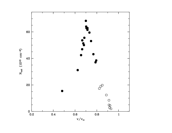
Figure 31: The variation of DAC column density as a function of central velocity in the Si iv resonance doublet of 19 Cep. The filled diamonds represent the strong DAC event in the August 1986 dataset; the open circles are the corresponding values for the DAC already at $v_{c}^{\mbox{\scriptsize asymp}}$ at the beginning of the 1986 campaign. Clearly, the DAC reaches a maximum in $N_{\mbox{\scriptsize col}}$ at 0.7 $v_{\infty}$.

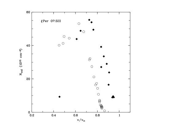
Figure 32: The variation of DAC column density as a function of central velocity in the Si iv resonance doublet of $\xi$ Per (October 1991). The open circles represent the “first” DAC event that reaches a lower $v_{c}^{\mbox{\scriptsize asymp}}$ than its successor (filled diamonds). Although the two curves reach the same maximum in $N_{\mbox{\scriptsize col}}$, they are shifted in velocity.

4.2 Short-term DAC evolution

The most striking property of the DAC phenomenon is the regularity in recurrence over many years. Time-series analyses show that the cyclical behaviour of DACs often results in a well-determined “wind” period. Although also other periods are found (some of them can be identified as harmonics of the principal period), the period with strongest power ($P_{\mbox{\scriptsize wind}}$) most often corresponds to the DAC recurrence timescale $t_{\mbox{\scriptsize rec}}$. In the case of $\zeta$ Ori $t_{\mbox{\scriptsize rec}}$ (1.6$\pm$0.2 day) is also detected in the power spectrum, but most power is associated with a period of about [6] days. In Table 2 we list $P_{\mbox{\scriptsize wind}}$ derived from the Si iv (or N v) resonance lines. The shorter the time span $\Delta t$ of the campaign, the less reliable the detected periods. When the period is comparable to or longer than $\Delta t$ it cannot be trusted. In Table 2 we marked these periods by putting them in between square brackets.

The DAC recurrence timescale is shorter for stars with a higher projected rotational velocity (Henrichs et al. HK88 (1988), Prinja Pr88 (1988)); this conclusion is supported by the results based on our larger sample. In Table 3 we compare the recurrence timescale of DACs with the estimated maximum rotation period of the star (the inclination of the stellar rotation axis is not known). An estimate for the stellar radius is obtained from Howarth & Prinja (HP89 (1989)). For all stars $t_{\mbox{\scriptsize rec}}$ is smaller than the maximum rotation period of the star. This supports the view that stellar rotation determines the characteristic timescale of (large-scale) wind variability in O-type stars. Whether $t_{\mbox{\scriptsize rec}}$ is equal to the stellar rotation period (or an integer fraction of this) will be discussed in section 5. Coordinated H$\alpha$ and UV observations of a few bright O stars have shown that $P_{\mbox{\scriptsize wind}}$ detected in UV resonance lines also appears in the H$\alpha$ line (Kaper et al. KH97 (1997)). On the basis of a large H$\alpha$ survey Kaper et al. (KF98 (1998)) demonstrate that the relation between $P_{\mbox{\scriptsize wind}}$ and the maximum rotation period also holds for this larger sample.

The variability of the inner regions of the stellar wind, where H$\alpha$ is formed, is directly linked to the DAC behaviour in UV resonance lines. This is confirmed by the detection of similar variability in subordinate UV lines in $\xi$ Per, HD 34656, and $\lambda$ Cep. In these stars, the subordinate N iv line at 1718 Å with P Cygni-type profile (and for $\lambda$ Cep also the He ii “Balmer$\alpha$” at 1640 Å) varies at low velocity in concert with the DACs (see also Henrichs et al. HK94 (1994) and Paper I). DACs have been detected in the N iv line of $\zeta$ Pup too (Prinja et al. PB92 (1992)). As these lines have to be formed in regions of higher density, this implies that material forming DACs must be present already close to the star (within a few $R_{\star}$).

Not only the cyclical appearance, but also the change in DAC central velocity per unit time is larger for stars with a shorter rotation period. This becomes apparent when one compares the DAC behaviour of the rapid rotators (e.g. $\xi$ Per, $\lambda$ Cep) with that in the most-likely slowly rotating stars (e.g. 19 Cep, 10 Lac). This suggests that the “acceleration” of DACs is not only a consequence of the line-forming region moving away from the star (where the wind speeds are higher); stellar rotation must play an important role too in explaining the acceleration timescale.

The variation of DAC column density as a function of their central velocity (i.e. time) is nicely demonstrated by the apparently slow rotator 19 Cep and the rapid rotator $\xi$ Per in Figs. 31 and 32, respectively. In both cases, the dependence of $N_{\mbox{\scriptsize col}}$ on $v_{c}$ resembles a parabolic function; a maximum in $N_{\mbox{\scriptsize col}}$ is reached half way. As $v_{\infty}$ we took the maximum $v_{c}^{\mbox{\scriptsize asymp}}$ we observed for the star (Table 1). It turns out that, for a given star, not all DACs have the same $v_{c}^{\mbox{\scriptsize asymp}}$. This can vary from campaign to campaign, or from event to event (e.g. $\xi$ Per, Fig. 32). Although the absolute velocities are different, the overall shape of the variation in $N_{\mbox{\scriptsize col}}$ is very similar, even for different stars.

As said before, the strength of a DAC varies from event to event. Sometimes, a weak absorption component disappears before reaching the wind terminal velocity. In several stars (e.g. $\xi$ Per and 68 Cyg) the stronger DACs are accompanied by weak absorption components separated by about a quarter of the DAC recurrence timescale. In most cases the two components merge when they arrive at the same velocity.

Table 3: DAC recurrence timescale compared to the estimated maximum stellar rotation period $P_{\mbox{\scriptsize max}}=$ 50.6 $(v\sin{i})^{-1}(R_{\star}/R_{\odot})$ days for the program stars. An estimate for the stellar radius is taken from Howarth & Prinja (HP89 (1989)). The stars are ordered according to $P_{\mbox{\rm max}}$. The last column lists the proposed stellar rotation period, based on our interpretation of the DAC behaviour.

Name	$v\sin{i}$	$R_{\star}$	$t_{\mbox{\scriptsize rec}}$	$P_{\mbox{\scriptsize max}}$	$P_{\mbox{\scriptsize rot}}$
	(km s-1)	($R_{\odot}$	(d)	(d)	(d)
68 Cyg	295	14	1.4	2.4	2.8
$\xi$ Per	204	11	2.0	2.7	4.0
$\lambda$ Cep	214	19	1.4	4.0	2.8
HD 34656	85	10	1.1	6.0	4.5
15 Mon	62	10	$>$4.5	8.2	$>$5
$\lambda$ Ori A	66	12	$\sim$4?	9.2	$>$4
19 Cep	90	18	$\sim$ 5	10.1	5 or 10
$\zeta$ Ori A	123	31	1.6	12.8	6?
10 Lac	31	9	6.8	14.7	7 or 14

In $\xi$ Per and 68 Cyg subsequent (strong) DACs alternate in asymptotic velocity. For $\xi$ Per the strong components reach $-$2050 or $-$2300 km s^-1. Since the lifetime of a strong DAC is longer than two days (the recurrence timescale), this results in “crossings” of successive components; they arrive at the same velocity, which does not mean that the material forming the two DACs is at the same physical location (though both in the line of sight). For 68 Cyg we identified two series of DACs, series A reaching an asymptotical velocity of $-$2450 km s^-1 and series B $-$2200 km s^-1. A difference with $\xi$ Per is that the time interval between series B and A is 0.5 d, which is much shorter than the recurrence timescale of 1.4 d (the distance in time between subsequent A’s or B’s, as well as pairs B A).

The difference between these sequences of DACs is visualized as follows:
series A $\rightarrow v_{\rm asymp}^{1}$ series B $\rightarrow v_{\rm asymp}^{2}$ $\xi$ Per A B A B A B A B A … 68 Cyg A B A B A B … HD 34656 A B B B A B B B A … time $\rightarrow$

The above mentioned DAC properties make up for the observed “pattern” of variability that is characteristic for the star. Sometimes it seems to be more complicated; e.g. in HD 34656 two different patterns can be recognized, a fast one and a slow one. More extended time series, like those obtained during the IUE MEGA campaign (Massa et al. MF95 (1995)), also indicate that the regular variability pattern is modulated by variations occuring over a longer, but eventually related timescale. A good example is provided by the MEGA campaign data on $\zeta$ Pup (Howarth et al. HP95 (1995)). These authors interpret the longer (5.2-day) period as the stellar rotation period; the shorter (19-hour) recurrence timescale of the DACs would, however, not be an integer fraction (6.5$\pm$0.9) of the rotation period. If the latter were true for this star, stellar rotation alone would not be sufficient to explain the cyclical recurrence of DACs.

4.3 Edge variability

In saturated P Cygni profiles wind variability manifests itself in significant shifts in velocity of the steep blue edge (cf. Paper I). In section 3 it is shown that close to the high-velocity edges of the UV resonance lines often a longer period is detected than the period exhibited by the DACs. We propose that the edge variability is directly related to the DAC behaviour. The observations suggest that the slow modulation of the high-velocity edges is the result of the fact that only the DACs with the highest asymptotic velocity have an impact on the position of the edge. The case of $\xi$ Per provides the strongest support to this interpretation: the edge variability has a period of about 4 days (i.e., twice the DAC recurrence timescale), while only one out of two DACs reaches an asymptotic velocity exceeding $-$2050 km s^-1.

The combination of a slow and a more rapid variability pattern (such as observed in HD 34656and $\zeta$ Pup) and the subsequent modulation in strength of the DACs might give rise to edge variability in saturated profiles on the timescale of the slow pattern. Therefore, only extended time series (such as those obtained in the IUE MEGA campaign, cf. Massa et al. MF95 (1995)) might enable confirmation of this conjecture.

4.4 Phase diagrams

The phase diagrams included in this paper show the variation of the sinusoid’s phase at the dominant wind variability period with position in the line. The observed decrease in phase towards higher velocities is due to the acceleration of the DACs through the line profile. This supports our view that $P_{\mbox{\scriptsize wind}}$ is equal to the DAC recurrence timescale. The large width of the DACs when they appear at low or intermediate velocity would explain the relatively small change in phase observed at these velocities.

Owocki et al. (OC95 (1995)) discuss the phase “bowing” discovered in the phase diagrams belonging to $P_{\mbox{\scriptsize wind}}$ detected in the B0.5 Ib star HD 64760 (Prinja et al. PM95 (1995), Fullerton et al. FM97 (1997)). Although, according to these authors, in this star $P_{\mbox{\scriptsize wind}}$ (1.2 or 2.4 d) is caused by a modulation in flux at low and intermediate velocities rather than by DACs, the decrease of phase towards both higher and lower velocities (which appears as a bow in the phase diagram) is a strong diagnostic of curved wind structures (like co-rotating interacting regions, section 5). DACs are detected at higher velocities in the resonance lines of HD 64760 and are variable on a timescale longer than $P_{\mbox{\scriptsize wind}}$.

The phase diagrams for the 2-day period detected in the $\xi$ Per October 1991 dataset clearly show evidence for phase bowing. A maximum in phase occurs around $-$1200  km s^-1, i.e. about the central velocity at which the DACs usually appear (Fig. 8). The maximum phase lag $\triangle\phi$ is about one radian, similar to the phase lag observed in HD 64760. The increasing strength of the DAC might explain the subsequent decrease in phase towards higher and lower velocities. The further acceleration and narrowing of the DACs is reflected by the increasing slope of the phase towards higher velocities. This description of the phase behaviour is only qualitative; detailed modeling of the phase diagram falls beyond the scope of this paper. An important difference with HD 64760 is that the DACs themselves seem to be responsible for the observed phase bowing.

Phase bowing is not evident in the phase diagrams for the other O stars in our sample. It has only been found in $\xi$ Per, which is perhaps not surprising, because the other stars in our sample do not exhibit such strong wind variability down to the lowest wind velocities.

4.5 Flux modulation and DAC behaviour

The “classical” picture we have of DAC behaviour, and which is supported by the observations analysed in this paper, is that broad absorption components appear at low velocity which evolve towards higher velocity while narrowing. The application of Fourier analyses resulted in the determination of well-constrained periods, not only at low velocity, but over the full width of the lines. To check the outcome of the Fourier analysis we constructed diagrams showing the variation of flux as a function of time in a each velocity bin. It indeed appears that the flux varies sinusoidally with time, especially at low and intermediate velocities. In some cases the Fourier analysis invokes an additional sinusoid to accommodate the weak precursor of the next DAC (resulting in the addition of a shorter-period sinusoid) or a gradual change (longer period). The latter occurs for example when two subsequent DACs reach a different asymptotic velocity.

The analysis of two spectroscopic time series of UV resonance lines of the B0.5 Ib supergiant HD 64760 lead Fullerton et al. (FM97 (1997)) to conclude that in this star a distinction can be made between a sinusoidal modulation in flux at low and intermediate wind velocities and variations due to the propagation of DACs at higher velocities. A 2.4-day (or 1.2-day) periodicity is connected with the modulation which clearly shows the occurrence of phase bowing; the DACs vary on a longer timescale. Thus, in HD 64760 two different kinds of wind variability are observed: flux modulation and DAC propagation. Because of the observed phase bowing, Fullerton et al. (FM97 (1997)) interpret the modulation to be due to CIRs, whereas the origin of the DACs is not clear.

Our results on $\xi$ Per indicate a different picture: in this star the flux modulation and phase bowing are caused by the DACs themselves. That the propagation of DACs leads to a sinusoidal modulation of the flux in a given velocity bin is due to the shape of the DACs, which can be accurately fit with an exponential Gaussian. At low velocity these gaussians have widths of several hundreds km/s. At high velocity they become very narrow. When the DAC moves through the resonance line, the flux in a given velocity bin changes gradually, following the Gaussian shape of the DAC. At high velocities, where the DACs are narrow, the flux changes more irregularly, because the DACs “pile up” at about the same asymptotic velocity before they vanish.

This might explain why the flux gradually changes when a DAC moves through a velocity bin, but not why this modulation is sinusoidal. In our interpretation, this is because not only the recurrence timescale, but also the acceleration timescale of the DAC is proportional to the rotation period of the star. Since these two timescales are identical, a sinusoidal shape of the flux versus time plots is expected. Thus, the DAC behaviour in O-star winds can result in a sinusoidal modulation of the flux in each velocity bin.

With our definition of the template, the maximum of the sinusoidal modulation corresponds to the “undisturbed, underlying wind profile”, so that all variations are by definition due to additional absorption. From the point of view of Fullerton et al. (FM97 (1997)), in the case of HD 64760 the template might be better defined as the zero-point of the modulation, i.e. the “average wind profile”. With such a template, it is not possible to model the DACs they observe in the resonance lines of HD 64760 at high velocity as absorption components, which is the reason for our approach.

4.6 Long-term variability

The O stars $\xi$ Per, 68 Cyg, 19 Cep, and $\lambda$ Cep were observed several times in the period 1986–1992. The variability pattern, characteristic for a given star, can be recognized from year to year, though detailed changes occur. The same wind variability timescale $P_{\mbox{\scriptsize wind}}$ is detected every year. Sometimes a different period gives the highest peak in the power spectrum ($\xi$ Per 1988 and 1989, 68 Cyg 1989), but this might be due to the short time coverage of these datasets. For $\lambda$ Cep there seems to be a clear difference between the observed variability timescale in October 1989, February 1991, and October 1991. In 1989 a period of [2.5$\pm$0.8 d] is dominant, in February 1991 a period of [4.3$\pm$1.2 d] (as well as 1.4$\pm$0.1 d), and in October 1991 a period of 1.4$\pm$0.2 d. If stellar rotation is setting the timescale of wind variability, one would not expect this timescale to vary from year to year. What could in principle vary is the number of features observed per rotation period. In the case of $\lambda$ Cep the difference in observed periods could be explained as different integer fractions of the stellar rotation period: 1.4, 2.8, 4.2 d; or 1.3, 2.6, 3.9 d. In section 5 we will address the point whether the DAC recurrence timescale can be used to determine the stellar rotation period.

Although the characteristic variability timescale remains the same, the DAC strengths and asymptotic velocities exhibit changes from campaign to campaign. The DAC behaviour in 68 Cyg seems to be the most constant over the years; clear differences are observed for $\xi$ Per (Fig. 6), 19 Cep, and $\lambda$ Cep. This indicates that the underlying clock might be the same, but that at least for some stars in our sample the pattern of large-scale structure in the stellar wind varies on a timescale of months to years.

5 Towards an interpretation

Several models have been put forward to explain the observed properties of DACs. The expansion of a high-density layer in the stellar wind (Henrichs et al. HH83 (1983)) gives a simple explanation for the time-dependent behaviour of DACs, but it gives no clue to the origin of the high-density layer. Underhill & Fahey (UF84 (1984)) tried to explain the existence and behaviour of DACs by postulating the existence of “closed” and “open” magnetic loops above the stellar surface from which parcels of gas are released in addition to a uniformly emitted steady stellar wind. A nice property of this model is that DACs are always expected to appear at the same rotational phase as long as the magnetic footpoints remain at the same location.

DACs are found at the same velocity in resonance lines formed by different ions (e.g. Lamers et al. LG82 (1982)); therefore, DACs most-likely originate from regions which have a higher density (or smaller velocity gradient) than the ambient wind. These regions have to be geometrically extended, because: (1) practically all O stars show DACs; (2) they have to cover a significant fraction of the stellar disk to be observable.

Stellar rotation plays a dominant role in setting the timescale of variability; a difference in flow time scale ($R_{\star}/v_{\infty}$) cannot explain the observed dependence on $v\sin{i}$. Not only the cyclical recurrence, but also the acceleration of DACs is faster for more rapidly rotating stars. This suggests that the DAC forming region rotates into and out of the line of sight. The observed increase and subsequent decrease of $N_{\mbox{\scriptsize col}}$ supports this picture (Figs. 31 and 32).

5.1 Corotating Interacting Regions and DACs

Most-promising is the Corotating Interacting Regions model proposed by Mullan (Mu84 (1984), Mu86 (1986)), in analogy with the corotating interacting regions in the solar wind which result from the interaction of fast and slow wind streams. Recently, this model has been worked out by Cranmer & Owocki (CO96 (1996)) who performed two-dimensional hydrodynamical simulations of corotating stream structure in the wind of a rotating O star. The corresponding spiral-shaped, large-scale structure through which the wind material is flowing, was proposed by Prinja & Howarth (PH88 (1988)) based on observations of 68 Cyg. Simultaneous ultraviolet and H$\alpha$ spectroscopy of a number of bright O stars included in this study strongly support the CIR model (Kaper et al. KH97 (1997), see also Fullerton et al. FM97 (1997)). Cranmer & Owocki (CO96 (1996)) conclude from their model that the DACs are not formed in the CIRs themselves, but originate in the so-called radiative-acoustic kinks trailing the CIRs. The strong velocity gradient related to this kink results in a relatively large contribution to the Sobolev optical depth. Kaper et al. (KH97 (1997)) show that a small phase lag might be present between the wind variations in the H$\alpha$ line with respect to those observed in the UV resonance lines; this would be consistent with the H$\alpha$ variations originating in the CIR and the DACs in the trailing kink.

Phase bowing suggests that the structures are curved, explaining why material at a given radial velocity rotates out of or into the line of sight first, followed by material moving at higher and lower velocities (Owocki et al. OC95 (1995), Cranmer & Owocki CO96 (1996)). All nine O stars with DACs show a decrease in phase towards higher velocities; only one ($\xi$ Per) also shows a lag in phase towards lower velocities. The location $r_{i}$ in the wind where the fast flow first meets the slow stream depends on the equatorial rotation speed $v_{\mbox{\scriptsize rot}}$ and the difference in (terminal) velocity between the fast and slow stream (Mullan Mu84 (1984)):

$$\frac{r_{i}}{R_{\star}}=1+\frac{\triangle\psi}{v_{\mbox{\scriptsize rot}}}\left[\frac{v_{\infty}^{\mbox{\scriptsize fast}}v_{\infty}^{\mbox{\scriptsize slow}}}{v_{\infty}^{\mbox{\scriptsize fast}}-v_{\infty}^{\mbox{\scriptsize slow}}}\right]$$ (11)

Inwards of $r_{i}$, the stellar wind might be rather smooth, so that variability is not detected at low wind velocities. Also, the “contrast” between the fast and slow stream (angular separation $\triangle\psi$ and $v_{\infty}^{\mbox{\scriptsize fast}}-v_{\infty}^{\mbox{\scriptsize slow}}$) is likely to vary from star to star. For large $r_{i}$ it might well be that only a decrease in phase towards higher velocities will be detected. Furthermore, the aspect angle might be an important factor; e.g. the decrease in phase towards lower velocities is only observed when the line of sight includes the equatorial plane.

The CIR model only works for rotating stars with emerging wind flows of different kinematic structure. Comparison between model and observations suggest that wind streams with relatively slow speed interact with the faster ambient wind, in stead of high-speed streams in a slow wind (Cranmer & Owocki CO96 (1996)). Therefore, the asymptotic velocity reached by DACs might be somewhat lower than the terminal velocity of the ambient wind. In some stars we measure systematically different values of $v_{c}^{\mbox{\scriptsize asymp}}$ from event to event. This might be due to a difference in aspect angle, contrast, or both.

5.2 The origin of CIRs: non-radial pulsations or surface magnetic fields?

In order to work, this model needs a certain structure imposed at the stellar surface to produce flows with different kinematical properties. Two physical mechanisms that in principle could cause fast and slow streams in the wind are: (i) non-radial pulsations (NRP), or (ii) surface magnetic fields. Henrichs (He84 (1984)) pointed out that the occurrence of DACs might be related to the presence of NRP at the stellar surface. NRP are detected (or suspected) in several O stars (cf. Baade Ba88 (1988), Fullerton et al. FG96 (1996)). The associated temperature and velocity fields (on the order of the sound speed) could be responsible for the modulation of the boundary conditions at the base of the radiation-driven wind.

Our working hypothesis is that the outflow properties at the base of the wind are influenced by a magnetic field anchored in the star, which results in regions with different outflow properties rotating with the star. The presence of magnetic fields in early-type stars is difficult to prove with direct observational methods. Magnetic fields with a strength of less than 100 Gauss are theoretically predicted (Maheswaran & Cassinelli MC92 (1992)), but not (yet) observable (Landstreet La92 (1992)). Recently, Stahl et al. (SK96 (1996)) argued that a surface magnetic field might be present in the O7 V star $\theta^{1}$ Ori C; phase-locked photospheric and stellar-wind variations strongly suggest that this star is an oblique magnetic rotator. An upper limit of 70 G for the (longitudinal) magnetic field strength of $\xi$ Per has been derived by Henrichs et al. (HD98 (1998)). Recent attempts to measure the longitudinal magnetic field strength in a sample of 10 fairly slowly rotating O stars by Mathys (Ma98 (1998)) and collaborators did not result in a definite detection (1$\sigma$ error bars of the order of 250–300 G). Some marginal measurements (between 2 and 3$\sigma$) suggest that weak fields might nevertheless be present, which could become detectable through a fairly modest improvement of the measurement accuracies.

Early-type stars are relatively short-lived objects and born out of interstellar matter that contains a magnetic field. The star with the strongest magnetic field known, “Babcock’s star” HD 215441, is a B3 V star with a surface dipole field strength of 34 kGauss (Babcock Ba60 (1960), Preston Pr71 (1971)). This demonstrates that early-type stars can have very strong magnetic fields (see also Bohlender Bo94 (1994)). These fields are expected to be frozen-in into the radiative envelopes of the stars (see, for example Mestel Me75 (1975)). Furthermore, the end-products of early-type stars are mostly neutron stars with a strong magnetic field, which strength can be predicted by assuming magnetic flux conservation during the collapse of the core and the presence of a surface magnetic field of strength 10–100 G in the progenitor. Alternative scenarios for the formation of neutron-star magnetic fields exist as well.

5.3 Can $t_{\mbox{\scriptsize rec}}$ be used to measure $P_{\mbox{\scriptsize rot}}$?

When we adopt the CIR model in combination with an anchored surface magnetic field to explain the presence and cyclical behaviour of DACs, the characteristic timescale of variability in the winds of O-type stars is the rotation period of the star. Our observations suggest that in several cases (e.g. $\xi$ Per and 68 Cyg where successive DACs have different asymptotical velocities) the rotation period of the star is more likely equal to twice (or an integral number times) the recurrence timescale of DACs. This means that DACs are not only a diagnostic for deriving the terminal velocity of a stellar wind, but they can in principle be used to derive the rotation period of the star. In Table 3 we list, based on the interpretation of the cyclical DAC behaviour, the best estimate for the rotation period of the star. Given an estimate of the stellar radius, the inclination of the rotation axis can thus be derived from $v\sin{i}$.

In two cases ($\xi$ Per and 68 Cyg) the proposed rotation period exceeds the estimated maximum rotation period. It is likely that these rapidly rotating stars (on the basis of the measured $v\sin{i}$) have a $\sin{i}$ value close to unity, and the radius of these stars could be slightly underestimated. For $\xi$ Per a radius of 15$R_{\odot}$ instead of 11$R_{\odot}$ would increase the maximum rotation period to 4 days (see Puls et al. PK96 (1996)). Walborn et al. (WN85 (1985)) note that $\xi$ Per is of luminosity class II instead of III which supports this conclusion. The uncertainty in the spectral class of 68 Cyg (denoted by the colon) also indicates that the estimated radius might not be accurate.

5.4 Summary and future work

The DAC behaviour in the UV resonance lines of a sample of 10 bright O stars has been analysed in detail. The cyclical appearance and subsequent evolution of DACs is interpreted in terms of a model invoking fast and slow streams which interact due to the rotation of the underlying star. The interacting regions (CIRs) corotate with the star while the wind material is flowing through them. The observations suggest that the stellar wind includes more than one CIR, most likely two (cf. Kaper et al. 1997). The curvature of the CIRs can in principle explain the observed phase behaviour (bowing), which is detected in one of the O stars in our sample. The wind variability periods we derive are a direct measure of the DAC recurrence timescales and, in our interpretation, equal to an integer fraction (most likely 1/2) of the stellar rotation period.

The key issue is the origin of the CIRs: are non-radial pulsations, surface magnetic fields, or other physical mechanisms responsible for the surface structure creating fast and slow wind streams? This is the subject of our current investigations.

- (1) Baade, D. 1988, in NASA/CNRS SP-497 “O, Of and Wolf-Rayet Stars”, Eds. Conti & Underhill, p. 137
- (2) Babcock, H.W. 1960, ApJ 132, 521
- (3) Bohlender, D. 1994, in IAU Symp. 162, Pulsation, Rotation and Mass Loss in Early-type stars, Eds. Balona, Henrichs, LeContel, p. 155
- (4) Conti, P.S., Ebbets, D. 1977, ApJ 213, 438
- (5) Cranmer, S.R., Owocki, S.P. 1996, ApJ 462, 469
- (6) Fullerton, A.W., Bolton, C.T., Garmany, C.D., et al. 1991, in Proc. ESO Workshop on Rapid variability of OB stars: Nature and diagnostic value, ed. D. Baade, p. 213
- (7) Fullerton, A.W., Gies, D.R., Bolton, C.T. 1996, ApJS 103, 475
- (8) Fullerton, A.W., Massa, D.L., Prinja, R.K., Owocki, S.P., Cranmer, S.R. 1997, A&A 327, 699
- (9) Gies, D.R., Kullavanijaya, A. 1988, ApJ 326, 813
- (10) Henrichs, H.F. 1984, in Proc. 4th European IUE Conf., Eds. Rolfe & Battrick (ESA SP-218), p. 43
- (11) Henrichs, H.F. 1988, in NASA/CNRS “O, Of and Wolf-Rayet Stars”, Eds. Conti & Underhill, p. 199
- (12) Henrichs, H.F., 1991, ESO Workshop on Rapid variability of OB stars: Nature and diagnostic value, Ed. D. Baade, p. 199
- (13) Henrichs, H.F., Hammerschlag-Hensberge, G., Howarth, I.D., Barr, P., 1983, ApJ 268, 807
- (14) Henrichs H.F., Kaper L., Zwarthoed G.A.A., 1988, in A Decade of UV Astronomy with the IUE Satellite (ESA SP-281), Vol.2, p.145
- (15) Henrichs, H.F., Kaper, L., Nichols, J. 1994, A&A 285, 565
- (16) Henrichs, H.F., de Jong, J.A., Nichols, J., et al. 1998, in Proc. “Ultraviolet astrophysics beyond the IUE final archive”, Eds. Wamsteker, González Riestra, Harris (ESA SP-413), p. 157
- (17) Howarth, I.D. 1992, in Proc. “Nonisotropic and Variable Outflows from Stars”, ASP Conf. Ser. 22, Eds. L. Drissen, C. Leitherer, A. Nota, p. 155
- (18) Howarth, I.D., Prinja R. 1989, ApJS 69, 527
- (19) Howarth, I.D., Bolton, C.T., Crowe, R.A., et al., 1993, ApJ 417, 338
- (20) Howarth, I.D., Prinja, R.K., Massa, D. 1995, ApJ 452, L65
- (21) Howarth, I.D., Smith, K.C. 1995, ApJ 439, 431
- (22) Kaper, L. 1998, in Proc. “Ultraviolet Astrophysics Beyond the IUE Final Archive”, ESA-SP 413, Eds. Wamsteker, González Riestra, Harris, p. 149
- (23) Kaper, L., Henrichs, H.F. 1994, Astr. Sp. Sc. 221, 115
- (24) Kaper, L., Henrichs, H.F., Nichols, J., et al. 1996, A&A Supp. Ser. 116, 1 (paper I)
- (25) Kaper, L., Henrichs, H.F., Fullerton, A.W., et al., 1997, A&A 327, 281
- (26) Kaper, L., Fullerton, A.W., Baade, D., et al. 1998, in Proc. ESO workshop “Cyclical variability in stellar winds”, Eds. Kaper, Fullerton, p. 103
- (27) Lamers, H.J.G.L.M., Gathier, R., Snow, T.P. 1982, ApJ 258, 186
- (28) Landstreet, J.D. 1992, A&AR 4, 35
- (29) Maheswaran, M., Cassinelli, J.P. 1992, ApJ 386, 695
- (30) Massa, D., Fullerton, A.W., Nichols, J.S., et al. 1995, ApJ, 452, L53
- (31) Mathys, G. 1998, in Proc. IAU Coll. 169, Eds. Wolf, Fullerton, Stahl, Springer Lecture Notes in Physics, in press
- (32) Mestel, L. 1975, in IAU Coll. 32: “Physics of Ap stars”, Univ. Sternwarte Wien, Vienna, Austria, p. 1
- (33) Mullan, D.J. 1984, ApJ 283, 303
- (34) Mullan, D.J. 1986, A&A 165, 157
- (35) Owocki, S.P., Cranmer, S.R., Fullerton, A.W. 1995, ApJ 453, L37
- (36) Peat, D.W. Pemberton, A.C., 1970, The Observatory 90, 141
- (37) Penny, L. 1996, ApJ 463, 737
- (38) Preston, G.W. 1971, PASP 83, 571
- (39) Prinja, R.K. 1988, MNRAS 231, 21P
- (40) Prinja, R.K. 1992, in Proc. “Nonisotropic and Variable Outflows from Stars”, ASP Conf. Ser. 22, Eds. L. Drissen, C. Leitherer, A. Nota, p. 177
- (41) Prinja, R.K. 1998, in Proc. ESO workshop “Cyclical variability in stellar winds”, Eds. Kaper, Fullerton, p. 92
- (42) Prinja, R.K, Balona, L.A., Bolton, C.T. et al. 1992, ApJ 390, 266
- (43) Prinja R.K., Barlow M.J., Howarth I.D. 1990, ApJ 361, 607
- (44) Prinja, R.K., Howarth, I.D. 1986, ApJS 61, 357
- (45) Prinja, R.K., Howarth, I.D., Henrichs, H.F. 1987, ApJ 317, 389
- (46) Prinja, R.K., Howarth, I.D. 1988, MNRAS 233, 123
- (47) Prinja, R.K., Massa, D., Fullerton, A.W. 1995, ApJ 452, L61
- (48) Puls, J., Kudritzki, R.-P., Herrero, A., et al. 1996, A&A 305, 171
- (49) Roberts, D,H, Lehar, J., Dreher, J.W. 1987, AJ 93, 968
- (50) Shore, S.N. Altner, B., Bolton, C.T. et al., 1993, ApJ 411, 864
- (51) Stahl, O., Kaufer, A., Rivinius, Th., et al. 1996, A&A 312, 539
- (52) Telting, J.H., Kaper, L., 1994 A&A 284, 515
- (53) Telting, J.H., Schrijvers, C. 1997, A&A 317, 723
- (54) Underhill, A.B., Fahey, R. 1984, ApJ 280, 712
- (55) Walborn, N.R. 1972, AJ 77, 312
- (56) Walborn N.R. 1973, AJ 78, 1067
- (57) Walborn, N.R., Nichols-Bohlin, J., Panek, R.J. 1985, NASA Ref. Pub. 1155