The X-ray Luminosity Function of Bright Clusters in the Local Universe

Abstract

We present the X-ray luminosity function (XLF) for clusters of galaxies derived from the RASS1 Bright Sample. The sample, selected from the $ROSAT$ All-Sky Survey in a region of 2.5 sr within the southern Galactic cap, contains 130 clusters with flux limits in the range $\sim 3-4\times 10^{-12}$ ergs cm^-2 s^-1 in the 0.5-2.0 keV band. A maximum-likelihood fit with a Schechter function of the XLF over the entire range of luminosities ($0.045-28.\times 10^{44}$ ergs s^-1), gives $\alpha=1.52^{+0.11}_{-0.11}$, $L_{*}=3.80^{+0.70}_{-0.55}\times 10^{44}$ ergs s^-1, and $A=5.07\pm 0.45\times 10^{-7}$ Mpc^-3 ($10^{44}$ ergs s^-1)^α-1. We investigate possible evolutionary effects within the sample, out to our redshift limit ($z\sim 0.3$), finding no evidence for evolution. Our results are in good agreement with other local estimates of the XLF, implying that this statistic for the local universe is now well determined. Comparison with XLFs for distant clusters ($0.3<z<0.6$), shows that no evolution is present for $L_{X}\lesssim 10^{44}$ ergs s^-1. However, we detect differences at the $3\sigma$ level, between our local XLF and the distant one estimated by Henry et al. for the EMSS sample. This difference is still present when considering the EMSS sample revised by Nichol et al.

1 Introduction

Clusters of galaxies have been extensively investigated as a powerful tool for cosmological studies. The X-ray luminosity function (XLF) is one of the most studied properties because it is related to the cluster mass function, gives information on the amplitude of the cosmic density fluctuation power spectrum and is sensitive to cluster evolution. Deep surveys covering small solid angles give information essentially on the faint-end of the XLF and on its redshift dependence (e.g., Henry et al. 1992, Rosati et al. 1998, Collins et al. 1997, Romer 1998, Jones et al. 1998). In contrast, shallow, wide-angle samples, allow the determination of the “local” (i.e., $z\lesssim 0.3$) XLF over the entire cluster luminosity range, which is crucial for studies of cluster evolution (e.g., Briel & Henry 1993, Ebeling et al. 1996, Ebeling et al. 1997). Early XLF studies of flux-limited samples compiled from $EXOSAT$ and $Einstein$ data (Edge et al. 1990, Gioia et al. 1990, Henry et al. 1992) showed evidence of negative cluster evolution at $z\gtrsim 0.1-0.2$ (Edge et al. 1990) or $z\gtrsim 0.3$ (Henry et al. 1992), whereas more recent work indicates that no evolution is present, at least for $z\lesssim 0.8$ and X-ray luminosities lower than $\sim 3\times 10^{44}$ ergs s^-1 (e.g., Burke et al. 1997, Rosati et al. 1998, Vikhlinin et al. 1998a).

To exploit the unique opportunity provided by the $ROSAT$ All-Sky Survey (RASS), we have constructed, from the first processing of the survey data, the RASS1 Bright Sample (De Grandi et al. 1999, hereafter Paper II) of clusters of galaxies, which covers a contiguous area of 8235 deg² in the southern hemisphere ($b_{II}<-20^{o},\delta<2^{o}.5$). This sample was constructed as part of an ESO Key Programme (Guzzo et al. 1995) aimed at surveying all the southern-sky RASS cluster candidates. This is now known as the REFLEX cluster survey (Böhringer et al. 1998), and it is currently nearing completion. Our sample contains 130 clusters with $ROSAT$ PSPC hard-band ($0.5-2.0$ keV) count rates higher than 0.25 counts s^-1 (corresponding to flux limits ranging from 3.05 to $4\times 10^{-12}$ ergs cm^-2 s^-1). A comprehensive discussion of the analysis of the X-ray data is given in De Grandi et al.(1997, hereafter Paper I), whereas the sample selection function and the estimation of the overall completeness and biases are presented in detail in Paper II. The relatively high flux limits (see Paper II), the large sky area covered, and the redshift distribution of the RASS1 Bright Sample make this sample particularly useful to study the local XLF out to $z\sim 0.3$. A first estimation of the XLF from a preliminary version of this sample, was presented by De Grandi (1996). In this Letter, we compute the XLF from the definitive sample described in Paper II. Presently, the only other sample selected from the RASS1 data with characteristics similar to those of our sample is the brightest cluster sample (BCS) of Ebeling et al. (1997, 1998). However, the selection procedures applied to compile the two samples are completely different with respect to both the selection procedure for the cluster candidates and the technique used to analyze the X-ray data. Throughout the Letter, we assume $H_{0}=50$ km s^-1 Mpc^-1 and $q_{0}=0.5$.

2 The Cluster Local XLF

The procedure to convert the observed counting rate of the clusters to luminosities was the following. First, source count rates in the 0.5-2.0 keV band were derived by using the Steepness Ratio Technique (SRT, Paper I), and converted to the corresponding un-absorbed total fluxes as described in Paper II. Next, we computed the cluster rest-frame luminosities for the 126 (out of 130) sources with available redshifts. We made $K$-corrections assuming that the typical spectra of clusters in the 0.5-2.0 keV energy band approximates a power law with energy index $\alpha=0.4$.

2.1 The method

The RASS1 Bright Sample has been obtained by performing a cut in SRT hard-band count rate at 0.25 counts s^-1 (see Paper II). Since different regions of the sky have different amounts of Galactic absorption, the cut in count rate translates into a range of flux limits varying between 3.05 and 4$\times 10^{-12}$ ergs cm^-2 s^-1 over the sampled area. The sky coverage, i.e., the amount of sky surveyed at the different flux limits, is shown in Figure 6 of Paper II. We have derived a non-parametric representation of the XLF of clusters based on the method described in detail by Avni & Bahcall (1980) for the coherent analysis of a set of independent samples. This method is a generalization of the classical $1/V_{max}$ estimator developed by Schmidt (1968). The volume $V_{a}$ that we use corresponds to the volume within which an object could have been detected above the flux limits of the sample. We have divided the observed range of luminosities in a number of bins and computed the differential XLF :

$${dn\over dL}(L)~{}=~{}{1\over\Delta L}\sum_{i=1}^{n_{j}}{1\over V_{a}(L_{i})}$$

where $n_{j}$ is the number of clusters in the $j^{th}$ bin and $V_{a}(L_{i})$ is the available volume corresponding to the luminosity $L_{i}$. The resulting XLF is shown in Figure 1; the $68\%$ error bars are determined by using the Marshall (1985) approximation.  Errors computed with simple Poissonian statistics are comparable to those computed with this approximation.

We have also assumed a parametric representation of the XLF and determined the parameters of the function through a maximum likelihood analysis. To this end, we have adopted a modified Schechter (1976) expression,

$${dn\over dL}(L)~{}=~{}AL^{-\alpha}\exp(-L/L_{*})~{},$$

characterized by the parameters $\alpha$ and $L_{*}$, which determine the shape of the function, and the normalization $A$. We have fitted the un-binned data to the Schechter function using an extension of the maximum likelihood method given in Murdoch, Crawford, & Jauncey (1973) and tested whether equation (2) is an adequate representation of the data with a Kolmogorov-Smirnov (K-S) test (details are given in the Appendix). To derive $\alpha$ and $L_{*}$, we have maximized the likelihood function ${\cal L}$ given in the Appendix. To compute the normalization factor $A$, we have required that the integral XLF $n(>L)$ of the Schechter model equal that observed for the minimum luminosity of the sample.

2.2 The results

The maximum likelihood method yielded best-fit parameters: $\alpha=1.52^{+0.11}_{-0.11}$, $L_{*}=3.80^{+0.70}_{-0.55}\times~{}10^{44}$ ergs s^-1 and $A=5.07\pm 0.45\times 10^{-7}$ Mpc^-3 (10⁴⁴ ergs s^-1)^α-1. The $68\%$ ($1\sigma$) confidence intervals for $\alpha$ and $L_{*}$ have been obtained by varying $2{\cal L}$ by 1 with respect to its maximum value (Maccacaro et al. 1988, and references therein). Errors for $A$ are derived from the uncertainty in the total number of clusters. A K-S test applied to the luminosity function (see Appendix) confirms that the Schechter model is an acceptable representation of the data. Indeed, we find a probability $P_{K-S}$ of exceeding the D statistic under the Null Hypothesis (i.e., “the data set comes from a distribution having the theoretical distribution”) equal to 0.59. The best fitting Schechter function is plotted in Figure 1 as a dashed line.

The XLF data points have not been corrected for the small, i.e., $\lesssim 10\%$, incompleteness. As discussed in Paper II, the main reason responsible for this incompleteness is, most likely, the bias against very extended sources (i.e. nearby clusters and groups). Therefore it should affect mainly the faint-end of the XLF (see also $\S 2.4$).

2.3 Test on evolutionary effects for z $\lesssim$ 0.3

To check for possible evolutionary effects at the moderate redshifts of our sample, we have divided the clusters into two redshift bins. In order to have subsamples with the same number of objects we have used as separator the median redshift (i.e., $z=0.0785$) of the total sample. In the inset of Figure 1 we report the $68\%$ and $90\%$ ($\Delta 2{\cal L}=2.3$ and $4.61$) confidence regions for the two parameters $\alpha$ and $L_{*}$ of the two XLFs derived with the same maximum likelihood procedure described above. We find that the best-fit $\alpha$, $L_{*}$ from the high-redshift subsample is enclosed within the $95.4\%$ region of the low-redshift subsample, whereas the best-fit $\alpha$, $L_{*}$ from the low-redshift subsample is enclosed within the $99.99\%$ region of the high-redshift subsample. From the overlap of the $90\%$ confidence regions we do not find evidence for evolution in our data. This is in agreement with what has been found in a similar redshift and luminosity range by Ebeling et al. (1997), and in other works on more distant cluster samples (e.g., Rosati et al. 1998).

2.4 Comparison with previous works

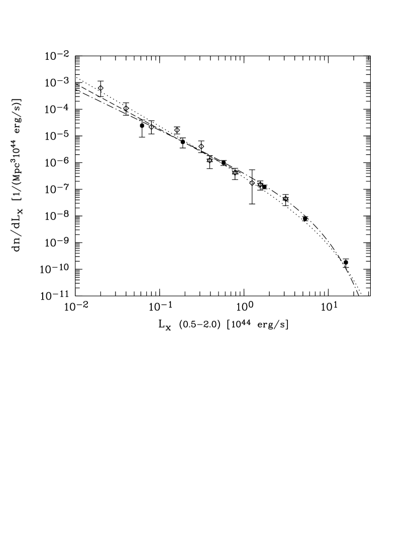
Figure 2: Cluster X-ray luminosity functions in the local universe. Independent determinations of the local XLF from the $ROSAT$ All-Sky Survey are shown: filled circles and the dot-dashed line represent the XLF and best-fitting Schechter function of the RASS1 Bright Sample (this work), the dotted line the BCS XLF (Ebeling et al. 1997), while the long-dashed line gives the XLF for poor clusters by Burns et al. (1996). Also reported are the XLF derived from the local part of deeper surveys: diamonds for the RDCS (Rosati et al. 1998) and stars for EMSS (Henry et al. 1992), in the $0.045<z<0.25$ and $0.14<z<0.2$ redshift ranges, respectively.

In Figure 2, we compare the RASS1 Bright Sample XLF with independent determinations of the local XLF compiled both from RASS1 data and from deeper X-ray surveys.

We consider first the BCS XLF (Ebeling et al. 1997), which is also well fitted in the 0.5-2.0 keV band by a Schechter function (eq. [2]). Inspection of Figure 2 shows that for $L\gtrsim 2\times 10^{43}$ ergs s^-1 the two XLFs are in good agreement. The difference between the XLFs below $\sim 2\times 10^{43}$ ergs s^-1 may reflect the different selection methods of the two samples. A K-S test between our data and the BCS best-fitting Schechter function over our whole luminosity range shows, however, that our data could have been drawn from the same population of the BCS sample ($P_{K-S}=0.11$). The second sample compiled from RASS1 data is the optically selected sample of poor clusters of galaxies from Burns et al. (1996). A K-S test performed between our data and their best-fitting power law XLF, after rescaling their parameters to $H_{0}=50$ km s^-1 Mpc^-1 and taking into account only the luminosity range in common with our sample, shows that the model agrees with our data ($P_{K-S}=0.67$).

As mentioned above, in Paper II we have estimated on overall incompleteness of our sample of $\sim 10\%$, affecting mainly the faint end of the XLF. A direct comparison of the BCS XLF best-fitting model with ours at the luminosity of $6.2\times 10^{42}$ ergs s^-1, representative of our lowest luminosity bin, shows a difference of about 13%. This result confirms that the incompleteness at faint luminosities must be indeed modest.

In Figure 2 we also compare our XLF with those derived from the EMSS (Henry et al. 1992) and RDCS (Rosati et al. 1998) samples in their nearest redshift shells, i.e., $0.14<z<0.2$ and $0.045<z<0.25$, respectively. We have converted EMSS luminosities from the $0.3-3.5$ keV to $0.5-2.0$ keV energy band assuming a Raymond-Smith thermal spectrum with temperature 6 keV and 0.3 solar abundances.  A two-sided K-S test between the EMSS data and ours, shows that the two distributions are not statistically different in the luminosity region where they overlap ($P_{K-S}=0.20$). A one-sided K-S test between our data and the best-fitting power law of the RDCS sample shows that our data is consistent with the RDCS XLF model ($P_{K-S}=0.40$). Both the EMSS and RDCS samples are selected purely by the X-ray properties of clusters. The good agreement between these independent determinations of the local XLF and our result, indicates that our cluster candidates pre-selection method, which is also based on optical information (Paper II), is well under control.

Finally, in Figure 3 we compare our XLF with those from the EMSS and RDCS, both computed for the $0.3<z<0.6$ redshift range, plus the RDCS XLF for $0.5<z<0.8$. Inspection of Figure 3 shows that the RDCS sample, covering a relatively small solid angle ($\sim 33$ deg²) with respect to the EMSS surveyed area (735 deg²), cannot probe the XLF above $2-3\times 10^{44}$ ergs s^-1, and that, for faint luminosities, no evolution seems to be present. On the contrary, the EMSS sample, being relatively shallower than the RDCS, probes mostly the bright-end of the XLF. We have compared the EMSS XLF in the $0.3<z<0.6$ redshift range with our XLF in the luminosity range covered by both functions ($0.74<L_{X}<8.67\times 10^{44}$ ergs s^-1). Using a two-sided K-S test between the EMSS data and ours, we find a difference of the two which is significant at the $3.3\sigma$ level ($P_{K-S}=8.3\times 10^{-4}$). This degree of evolution is similar to what was found in Henry et al. (1992). Recently, Nichol et al. (1997) have revised the EMSS cluster sample, using both new X-ray and optical data. A K-S test between the revised EMSS data and ours in the same luminosity range as above gives $P_{K-S}=7.7\times 10^{-4}$, indicating that the two XLFs are still different at the $3.3\sigma$ level. Recently, Reichart et al. (1998) re-examined the EMSS sample and noted the deficiency of bright ($L_{X}>L_{*}$) high redshift ($z>0.3$) systems. Also, Vikhlinin et al. (1998a), studying a sample of clusters detected in a 160 deg² survey of $ROSAT$ PSPC fields (Vikhlinin et al. 1998b), find evidences of a deficit of high luminosity distant clusters at more than $99.5\%$ confidence. As noted by the authors, their sample was selected by using photometric redshifts, and the optical spectroscopic identification of the X-ray sources is still in progress.

Appendix A Appendix

We extend here the maximum likelihood method discussed in Crawford, Jauncey, & Murdoch (1970) and Murdoch et al. (1973), which works on the un-binned data distribution, in order to estimate the best-fitting parameters of the X-ray luminosity function when the assumed model is a Schechter function (eq. [2]). For consistency reasons, we adopt essentially the same notation of Murdoch et al. (1973). We describe the treatment of the multi-volume case for a flux-limited sample in an error-free situation. Since the sample discussed in this work is characterized by a set of flux-limits, the maximum volume of each source is the available volume $V_{a}$, as described in Avni & Bahcall (1980).

In general, if one considers sources within the volume $V_{a_{j}}$ having luminosities in the range between $L_{0j}$ and $L_{uj}$, then the probability density $P(L_{ij})$ for the $i$th source of luminosity $L_{ij}$ in the volume $j$ is given by

$$P(L_{ij})={V_{a_{j}}\over K}\exp(-L_{ij}/L_{*})L_{ij}^{-\alpha},$$

where the normalization factor $K$ is computed by integrating over all the volumes $\sum_{j}\int^{L_{uj}}_{L_{0j}}P(L_{ij})dL_{ij}\equiv 1$, which gives

$$K=\sum_{j}V_{a_{j}}\int^{L_{uj}}_{L_{0j}}\exp(-L_{ij}/L_{*})L_{ij}^{-\alpha}dL_{ij}.$$

The maximum likelihood method consists in maximizing the probability density of occurrence of the observed values of $L_{ij}$, given the assumed Schechter function. Following Murdoch et al. (1973), this reduces to maximizing the likelihood function ${\cal L}=\Sigma_{i}\Sigma_{j}lnP(L_{ij})$, where the summation is over all of the observed luminosities. Hence,

$${\cal L}=\sum_{j}m_{j}\ln V_{a_{j}}-M\ln K-{1\over L_{*}}\sum_{i}\sum_{j}L_{ij}-\alpha\sum_{i}\sum_{j}\ln L_{ij},$$

where $m_{j}$ is the number of sources observed in the volume $V_{a_{j}}$ and $M=\Sigma_{j}m_{j}$ is the total number of sources in the sample. The maximum value of ${\cal L}$ is found by constructing a grid of values of the likelihood function by varying the parameters $\alpha$ and $L_{*}$. The same grid of values is used to compute the uncertainties on the two parameters as a function of the confidence level.

Finally, to test if the Schechter function is an adequate representation of the data, we use a K-S test that can be applied to unbinned data. In this case, we transform the assumed function into a cumulative distribution ranging from 0 to 1 by computing

$$y_{i}(L_{ij}^{\prime})=\sum_{j}\int^{L_{ij}^{\prime}}_{L_{0j}}P(L_{ij})dL_{ij}={\sum_{j}V_{a_{j}}\int^{L_{ij}^{\prime}}_{L_{0j}}\exp(-L_{ij}/L_{*})L_{ij}^{-\alpha}dL_{ij}\over{\sum_{j}V_{a_{j}}\int^{L_{uj}}_{L_{0j}}\exp(-L_{ij}/L_{*})L_{ij}^{-\alpha}dL_{ij}}}$$

and then examining the observed $y_{i}$ distribution for departure from the expected distribution through the K-S test.

Figure 1: X-ray luminosity function for the RASS1 Bright Sample of clusters of galaxies. Dots and error bars represent the differential XLF, whereas the long-dashed line is the best-fitting Schechter function estimated with a maximum likelihood method from the unbinned data distribution (see the Appendix). The inset shows the $68\%$ and $90\%$ confidence regions for $\alpha$ and $L_{*}$ (which is in units of $10^{44}$ ergs s^-1) in two different redshift bins: dotted and solid lines refer to the $z<z_{median}$ and $z>z_{median}$ redshift ranges, respectively. Crosses refer to the best-fit parameters for the two subsamples, whereas the asterisk refers to the total sample.

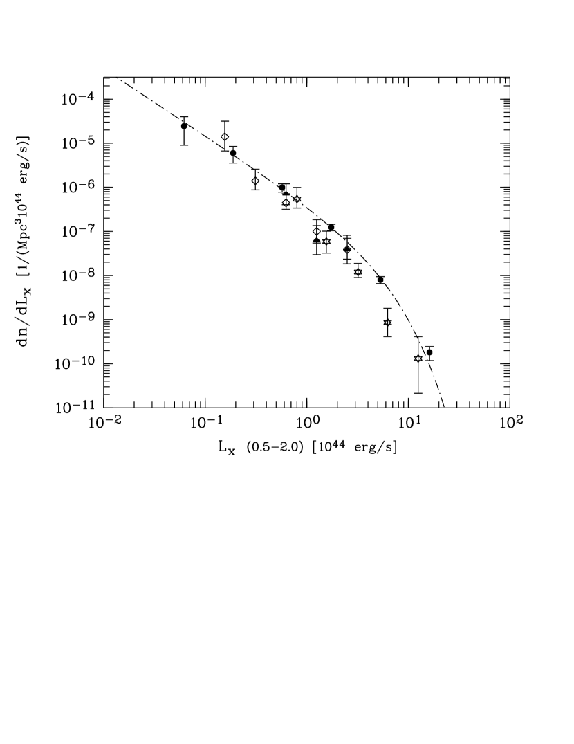
Figure 3: Comparison of the local and distant cluster X-ray luminosity functions. Filled circles and the dot-dashed line represent the local XLF and the best-fitting Schechter function of the RASS1 Bright Sample (this work). Diamonds and stars are from the RDCS and the EMSS, both computed in the $0.3<z<0.6$ redshift range, while filled triangles give the RDCS XLF for $0.5<z<0.85$.

References

- (1) Avni, Y. & Bahcall, J.N., 1980, ApJ, 235, 694
- (2) Böhringer, H., et al. 1998, ESO Messenger, 94, 21
- (3) Briel, U. G. & Henry, J. P., 1993, A&A, 278, 379
- (4) Burke, D. J., Collins, C. A., Sharples, R. M., Romer, A. K., Holden, B. P., Nichol, R. C. 1997, ApJ, 488, L83
- (5) Burns, J. O., Ledlow, M. J., Loken, C., Klypin, A., Voges, W., Bryan, G. L., Norman, M. L., & White, R. A. 1996, ApJ, 467, L49
- (6) Collins, C.A., Burke, A., Romer, A.K., Sharples, R. M., Nichol, R.C., 1997, ApJ, 479, L117
- (7) Crawford, D. F., Jauncey, D. L. & Murdoch, H. S. 1970, ApJ, 162, 405
- (8) De Grandi, S. 1996, in MPE Rep. 263, Proc. Röntgenstrahlung from the Universe, ed. H. U. Zimmermann, J. Trümper & H. Yorke (Munich:MPE), 577
- (9) De Grandi, S., Molendi, S., Böhringer, H., Chincarini, G. & Voges, W. 1997, ApJ, 486, 738 (Paper I)
- (10) De Grandi, S., Böhringer, H., Guzzo, L., Molendi, S., Chincarini, G., Collins, C., Cruddace, R., Neumann, D., Schindler, S., Schuecker, P., & Voges, W. 1999, ApJ, 514, in press (Paper II)
- (11) Ebeling, H., Edge, A. C., Böhringer, H., Allen, S. W., Crawford, C. S., Fabian, A. C., Voges, W., Huchra, J.P. 1998, MNRAS, 301, 881
- (12) Ebeling, H., Edge, A. C., Fabian, A. C., Allen, S. W., Crawford, C. S., Böhringer, H. 1997, ApJ, 479, L101
- (13) Ebeling, H., Voges, W., Böhringer, H., Edge, A. C., Huchra, J. P., Briel, U. G. 1996, MNRAS, 281, 799
- (14) Edge, A. C., Stewart, G. C., Fabian, A. C. and Arnaud, K. A., 1990, MNRAS, 245, 559
- (15) Gioia, I. M., Henry, J. P., Maccacaro, T., Morris, S. L. & Stocke, J. T. 1990, ApJ, 357, L35
- (16) Guzzo, L. et al. 1995, Proc. Wide Field Spectroscopy and the Distant Universe, ed. Maddox S. J. & Aragon-Salamanca A. (Singapore: World Scientific), 205
- (17) Henry, J. P., Gioia, I. M., Maccacaro, T., Morris, S. L., Stocke, J. T., & Wolter, A. 1992, ApJ, 386, 408
- (18) Jones, L. R., Scharf, C., Ebeling, H., Perlman, E., Wegner, C., Malkan, M. and Harner, D., 1998, ApJ, 495, 100
- (19) Maccacaro, T., Gioia, I. M., Wolter, A., Zamorani, G. and Stocke, J. T., 1988, ApJ, 326, 680
- (20) Marshall, H. L., 1985, ApJ, 299, 109
- (21) Murdoch, H. S., Crawford, D. F. & Jauncey, D. L. 1973, ApJ, 183, 1
- (22) Nichol, R. C., Holden, B. P., Romer, A. K., Ulmer, M. P., Burke, D. J., Collins, C. A. 1997, ApJ, 481, 644
- (23) Reichart, D. E., Nichol, R. C., Castander, F. J., Burke, D. J., Romer, A. K., Holden, B. P., Collins, C. A., Ulmer, M. P., preprint astro-ph/9802153
- (24) Romer, A. K., preprint astro-ph/9809198
- (25) Rosati, P., Della Ceca, R., Norman, C. & Giacconi, R. 1998, ApJ, 492, L21
- (26) Schechter, P. 1976, ApJ, 203, 297
- (27) Schmidt, M. 1968, ApJ, 151, 393
- (28) Vikhlinin, A., McNamara, B. R., Forman, W., Jones, C., Quintana, H. & Hornstrup, A. 1998a, ApJ, 498, L41
- (29) Vikhlinin, A., McNamara, B. R., Forman, W., Jones, C., Quintana, H. & Hornstrup, A. 1998b, ApJ, 502, 558