Cosmological Constraints from the Clustering Properties of the $X$–Ray Brightest Abell–type Cluster Sample

Abstract

We present an analysis of the 2–point correlation function, $\xi(r)$, of the $X$–ray Brightest Abell–type Cluster sample (XBACs; Ebeling et al. 1996) and of the cosmological constraints that it provides. If $\xi(r)$ is modelled as a power–law, $\xi(r)=(r_{0}/r)^{\gamma}$, we find $r_{0}\simeq 26.0\pm 4.5$ $h^{-1}{\mathrm{Mpc}}~{}$and $\gamma\simeq 2.0\pm 0.4$, with errors corresponding to 2$\sigma$ uncertainties for one significant fitting parameter. As a general feature, $\xi(r)$ is found to remain positive up to $r\simeq 50$–55 $h^{-1}{\mathrm{Mpc}}~{}$, after which it declines and crosses zero. Only a marginal increase of the correlation amplitude is found as the flux limit is increased from $5\times 10^{-12}$ erg s^-1 cm^-2 to $12\times 10^{-12}$ erg s^-1 cm^-2, thus indicating a weak dependence of the correlation amplitude on the cluster $X$–ray luminosity. Furthermore, we present a method to predict correlation functions for flux–limited $X$–ray cluster samples from cosmological models. The method is based on the analytical recipe by Mo & White (1996) and on an empirical approach to convert cluster fluxes into masses. We use a maximum–likelihood method to place constraints on the model parameter space from the XBACs $\xi(r)$. For scale–free primordial spectra, we find that the shape parameter of the power spectrum is determined to lie in the $2\sigma$ range $0.05\raise-2.0pt\hbox{\hbox to0.0pt{\hbox{$\sim$}\hss}\raise 5.0pt\hbox{$<$}\ }\Gamma\raise-2.0pt\hbox{\hbox to0.0pt{\hbox{$\sim$}\hss}\raise 5.0pt\hbox{$<$}\ }0.20$. As for the amplitude of the power–spectrum, we find $\sigma_{8}\simeq 0.4$–0.8 for $\Omega_{0}=1$ and $\sigma_{8}\simeq 0.8$–2.0 for $\Omega_{0}=0.3$. The latter result is in complete agreement with, although less constraining than, results based on the local cluster abundance.

1 Introduction

Galaxy clusters have been recognised since a long time as extremely useful tracers of the large–scale structure of the Universe. Being the largest virialized cosmic structures, they can be detected rather unambiguously up to very large distances. Furthermore, their distribution traces scales which have not yet undergone the non–linear phase of gravitational clustering, therefore simplifying their connection to the initial conditions of cosmic structure formation.

So far, most of the studies of the cluster distribution have relied on optical samples like the Abell/ACO one (Abell 1958; Abell Corwin & Olowin 1989), the APM sample (Dalton et al. 1994) and the EDCC sample (Collins et al. 1995). A general result from such analyses is that the two–point cluster correlation function is well approximated by a power–law, $\xi(r)=(r_{0}/r)^{\gamma}$, with $\gamma\simeq 1.8$–2. The measured correlation length $r_{0}$, range in the interval $r_{0}\simeq 15$–25 $h^{-1}{\mathrm{Mpc}}~{}$, depending on the analysed sample and/or on the cluster richness (see, e.g., Bahcall & West 1992, Croft et al. 1997; and references therein).

A serious problem arising in optical cluster compilations is the spurious enhancement of the cluster richness in high density environments which can also cause inherently poor clusters or groups to appear rich enough to be included in the sample (e.g. van Haarlem, Frenk & White 1997). This led several authors to cast doubts about the reliability of the clustering analysis of Abell/ACO clusters, whose correlation function could be artificially enhanced by such projection effects (cf. Sutherland 1988; Dekel et al. 1989; Peacock & West 1992; see, however, Jing, Plionis & Valdarnini 1992 for an alternative view). Although samples like the APM and the EDCC have been designed with the purpose of minimising projection effects, they could still be present at some level (e.g., Collins et al. 1995).

This calls for the need to confirm results based on optical samples by studying other cluster compilations which are free of the above mentioned biases. $X$–ray selected cluster samples are ideally suited for this purpose. Indeed, since the $X$–ray emissivity of the intra–cluster medium (ICM) is proportional to the square of the gas density, cluster emission is strongly peaked at the centre, so as to make the impact of projection effects almost negligible. Important analyses of the large-scale distribution of relatively small $X$–ray cluster samples have already been performed in recent years (cf. Romer et al. 1994; Nichol, Briel & Henry 1994, Guzzo et al. 1995).

More recently, the $X$–Ray Brightest Abell Cluster sample (XBACs, hereafter; Ebeling et al. 1996) has been compiled from cross–correlating the ROSAT all–sky $X$–ray survey with the Abell/ACO cluster sample (for further details see their Section 4). Although it is not purely $X$–ray selected, the inclusion of only those Abell/ACO clusters that have an extended and significant $X$-ray emission suppress the biases affecting the purely optical sample (cf. Ebeling et al. 1996, Plionis & Kolokotronis 1998; PK98, hereafter). The XBACs provides for the first time a whole sky, flux–limited sample of $X$–ray galaxy clusters. This sample has been analysed by PK98 with the aim of investigating the local acceleration field and by Abadi, Lambas & Muriel (1998) to study the cluster 2–point correlation function (see also Kolokotronis 1998).

In this paper, we present a new analysis of the correlation function for the XBACs cluster distribution, with the specific aim of investigating its implication on cosmological models for large–scale structure formation. In this context, a great advantage in using galaxy clusters, instead of galaxies, as tracers of the large-scale structure lies in their less ambiguous connection with the underlying dark matter (DM) density fluctuations. As for $X$–ray clusters, the problem of understanding their biasing with respect to the DM distribution requires a suitable description of the connection between the $X$–ray luminosity and the mass of the virialized DM halo hosting the emitting gas. This problem, although not of trivial solution, is much more affordable, both from a numerical and an analytical point of view, than an accurate understanding of galaxy formation and evolutionary processes.

In what follows, we will use the analytical approach by Mo & White (1996) to describe the correlation function for the distribution of clusters, which are identified as virialized halos of a given mass. This recipe in itself is not enough to compare model predictions with XBACs data, since the XBACs cluster selection is clearly not based on a mass threshold criterion. For this reason, we will resort to a phenomelogical approach to connect cluster masses to observed $X$–ray fluxes (cf. also Borgani et al. 1998). Although our analysis is entirely based on a sample of local clusters, all the formalism that we will present is developed to treat the cluster distribution at a generic redshift. Therefore, our analysis method is amenable to be directly applied to obtain cosmological constraints from future deep surveys of galaxy clusters.

The structure of the paper can be summarised as follows. In Section 2 we provide a short description of the XBACs sample and of the results of the $\xi(r)$ analysis. We describe in Section 3 how to compute cluster correlations for an $X$–ray flux–limited sample from cosmological models, which are characterised by a given power–spectrum of density fluctuations and by the geometry of the Friedmann background. The method to compare model predictions to real data analysis is discussed in Section 4. In Section 5 we briefly discuss such results and draw the main conclusions.

2 Correlation analysis of XBACS

2.1 The XBACs sample

The XBACs sample consists of the X–ray brightest Abell/ACO clusters that have been detected in the ROSAT all sky survey (RASS; Trümper 1990; Voges 1992) for fluxes above $S_{\rm lim}=5\times 10^{-12}\,$erg s${}^{-1}\,$cm^-2 ([0.1–2.4] keV band) with redshifts limited by $z\leq 0.2$. The sample contains 253 clusters and thus it is the largest X–ray flux–limited cluster sample to date (though not entirely X–ray selected). The X–ray fluxes measured initially by the Standard Analysis Software System (SASS) point source detection algorithm are superseded by Voronoi Tessellation Percolation (VTP) measurements, which better account for the extended nature of the emission. In addition, the difficulty of the SASS algorithm to actually detect nearby X–ray emission has been mostly corrected by running VTP on the RASS fields centred on the optical positions of all nearby Abell/ACO clusters ($z\leq\,$0.05) irrespective of whether or not they are detected by SASS. Ebeling et al. (1996) estimate, after a careful analysis of possible selection effects and biases that the overall completeness of this X–ray sample is $\raise-2.0pt\hbox{\hbox to0.0pt{\hbox{$\sim$}\hss}\raise 5.0pt\hbox{$>$}\ }80\%$ at the above flux limit.

An extended discussion of the possible XBACs systematic effects is presented in PK98. Here we present only a brief summary.

The known volume incompleteness effect, as a function of distance, for the richness class R=0 Abell/ACO clusters, is not present in the XBACs sample (Ebeling et al. 1996). Indeed, thanks to its flux–limited property, the sample contains at large distances the inherently brighter and thus richer Abell/ACO clusters, for which there is no volume incompleteness. Furthermore the significant distance dependent density variations, which are most probably due to the higher sensitivity of the ACO IIIa-J emulsion plates, between the northern Abell and southern ACO parts of the combined optical cluster sample (cf. Batuski et al. 1989; Scaramella et al. 1991; Plionis & Valdarnini 1991) has been corrected for in the XBAC sample (see details in PK98).

The main remaining biases that need to be quantified for the correlation analysis are the redshift selection function, which depends on the XBACs luminosity function and flux limit, and the Galactic absorption latitude selection function, which has been found to be consistent with a cosecant law of the form

$$P(|b|)=\mbox{dex}\;\left[\alpha\left(1-\csc|b|\right)\right]$$ (1)

with $\alpha\approx 0.3$ for the Abell sample (Bahcall & Soneira 1983; Postman et al. 1989) and $\alpha\approx 0.2$ for the ACO sample (Batuski et al. 1989). In the following we will restrict our analysis to clusters having $|b|\geq 30^{\circ}$.

The XBACs redshift distribution, in the form of an $N(r)$ plot, corrected for Galactic absorption, can be seen in Figure 1. We have also plotted as a continuous line the predicted radial distribution function based on the XBACs luminosity function (see references in PK98) and the $5\times 10^{-12}$ erg s^-1 cm^-2 flux limit.

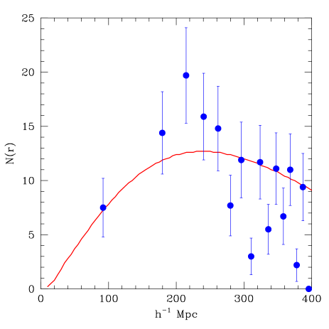
Figure 1: The XBACs radial distribution function and its Poisson uncertainty (filled circles). The predicted distribution based on the XBACs luminosity function estimated by PK98 is shown as a continuous line.

Note that redshifts are converted into luminosity distances according to

$$d_{L}(z)\,=\,{c\over H_{0}}\,r(z)\,(1+z)$$ (2)

where $H_{0}=100\,h$ km s${-1}$ Mpc^-1 is the Hubble constant and

$$r(z) = \int_{0}^{z}dz\,E^{-1}(z)~{}~{}~{};~{}~{}~{}\Omega_{\Lambda}=1-\Omega_{0}$$

$$r(z) = {2\left[\Omega_{0}z+(2-\Omega_{0})\,(1-\sqrt{1+\Omega_{0}z})\right]\over\Omega_{0}^{2}(1+z)}~{};~{}\Omega_{\Lambda}=0\,.$$ (3)

Here $E(z)=[(1+z)^{3}\Omega_{0}+\Omega_{\Lambda}]^{1/2}$ for a flat Universe (e.g., Peebles 1993). In what follows, results and comparisons with models will be presented for two values of the density parameter; $\Omega_{0}=1$ and 0.3, with and without a cosmological constant term ($\Omega_{\Lambda}=\Lambda/3H_{0}^{2}$) to restore spatial flatness.

2.2 The $\xi(r)$ estimate

We estimate the 2-point correlation function for XBACs using the following estimator:

$$1+\xi(r)=2\,\frac{N_{cc}}{\langle N_{cr}\rangle}$$ (4)

where $N_{cc}$ is the number of cluster pairs in the interval $[r-\delta r,r+\delta r]$ and $\langle N_{cr}\rangle$ is the average, over 10,000 random simulations with the same boundaries, redshift and galactic latitude selection functions, cluster-random pairs in the same separation interval. We have evaluated $\xi(r)$ in logarithmic intervals with constant logarithmic amplitude $\Delta\sim 0.1$. We estimate the variance of $\xi(r)$ by using the analytical approximation to the bootstrap errors (Mo, Jing & Börner 1992) which has been shown to reproduce fairly accurately the actual bootstrap variance:

$$\sigma_{\xi}^{2}\simeq 3\times\sigma_{qP}^{2}=3\times{1+\xi(r)\over N_{cc}(r)}\,,$$ (5)

where $\sigma^{2}_{qP}$ is the quasi–Poisson variance.

Table 1: Results for the three samples. Column 2: flux limits (units of $10^{-12}\,$erg s${}^{-1}\,$cm^-2); Column 3: number of clusters; Column 4: correlation length and 2$\sigma$ uncertainty (units of $h^{-1}{\mathrm{Mpc}}~{}$); Column 5: slope of $\xi(r)$ and 2$\sigma$ uncertainty.

	$S_{lim}$	No. of clusters	$r_{0}$	$\gamma$	$\chi^{2}_{min}$
(a)	5	203	$26.0^{+4.1}_{-4.7}$	$1.98^{+0.35}_{-0.53}$	3.9
(b)	8	112	$25.9^{+5.2}_{-6.6}$	$2.02^{+0.43}_{-0.76}$	3.6
(c)	12	67	$27.5^{+8.7}_{-12.8}$	$1.94^{+0.85}_{-1.52}$	5.8

We apply the correlation analysis to the whole sample ($z\raise-2.0pt\hbox{\hbox to0.0pt{\hbox{$\sim$}\hss}\raise 5.0pt\hbox{$<$}\ }0.2$), with $S_{\rm lim}=5\times 10^{-12}\,$erg s${}^{-1}\,$cm^-2 [sample (a)] and to two other subsamples with $S_{\rm lim}=8\times 10^{-12}\,$erg s${}^{-1}\,$cm^-2 and $S_{\rm lim}=12\times 10^{-12}\,$erg s${}^{-1}\,$cm^-2 [samples (b) and (c), respectively]. The total number of clusters in each sample is reported in Table 1.

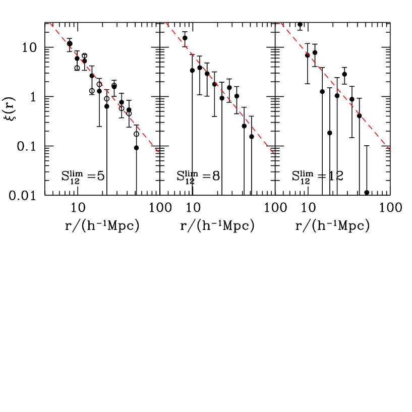
Figure 2: The 2–point correlation function for samples (a), (b) and (c), by assuming $\Omega_{0}=1$ to convert redshifts into distances (cf. eqs.(2) and (3). Errorbars correspond to 1$\sigma$ bootstrap uncertainties. Open circles for the (a) sample corresponds to the open $\Omega_{0}=0.3$ case. The dashed lines corresponds to the best fitting power–law expressions, $\xi(r)=(r_{0}/r)^{\gamma}$, whose parameters are reported in Table 1.

The resulting $\xi(r)$, using $\Omega_{0}=1$ in eq.(3), for the three samples are plotted in Figure 2. Only for sample (a) we show the $\xi(r)$ by using $\Omega_{0}=0.3$. Due to the limited depth of XBACs no significant differences are found between these two cases. For all the three samples $\xi(r)$ is positive up to $r\simeq 50$ $h^{-1}{\mathrm{Mpc}}~{}$, after which it declines and crosses zero at about 50 - 55 $h^{-1}{\mathrm{Mpc}}~{}$. This result agrees with that found for optical Abell/ACO cluster samples (e.g., Klypin & Rhee 1994) and confirms that the cluster distribution requires a substantial amount of large–scale coherence of cosmic density fluctuations.

The dashed lines in the plots represent the best–fitting power law model, $\xi(r)=(r_{0}/r)^{\gamma}$, which is determined through a $\chi^{2}$–minimisation ($\chi^{2}_{min}$ hereafter) procedure, assuming a Gaussian distribution for $\sigma_{\xi}$. The fit for the (c) sample has been performed only including bins with $r>10$ $h^{-1}{\mathrm{Mpc}}~{}$, so as to exclude the anomalous high–correlation signal coming from the smallest scales. On a more quantitative ground, Figure 3 shows the iso–$\Delta\chi^{2}$ contours ($\Delta\chi^{2}=\chi^{2}-\chi^{2}_{min}$, with $\chi^{2}_{min}$ being the absolute minimum value of $\chi^{2}$) in the $r_{0}$–$\gamma$ plane. Strictly speaking, $\xi(r)$ estimates in different bins are not independent of each other, since each cluster contributes to pairs at different separations. The contours correspond to $1\sigma$ and $2\sigma$ uncertainties for two significant parameters and correspond to $\Delta\chi^{2}=2.30$ and 6.17, respectively. Figure 4 shows the variation of $\Delta\chi^{2}$ around the best–fitting value of each of the two parameters, once we marginalise with respect to the other parameter. The best fitting values for $r_{0}$ and $\gamma$, along with the $2\sigma$ uncertainty for one significant fitting parameter are also reported in Table 1. It turns out that increasing $S_{lim}$ the correlation length only marginally increases. As long as a correlation exists between cluster $X$–ray luminosity and richness, this result implies only a mild dependence of the clustering strength on the cluster richness (see also Croft et al. 1997).

Results for sample (a) can be compared with those obtained by Abadi et al. (1998) for the same sample. They find a somewhat lower correlation amplitude, with $r_{0}\simeq 21$ $h^{-1}{\mathrm{Mpc}}~{}$and a similar $\gamma$ value but with much smaller uncertainties (cf. their Fig. 4). We are not sure why their estimate of $r_{0}$ is lower than ours. However, the rather large difference in the uncertainties is entirely due to their assumption of Poissonian errors for $\xi(r)$. We verified that repeating our analysis assuming quasi–Poisson errors (cf. the upper right panel in Fig. 3), the contours in the $r_{0}$–$\gamma$ plane shrinks into a much smaller size, comparable to that reported by Abadi et al. (1998).

3 Predicting correlations for flux–limited samples

In this section we introduce the formalism to compute model $\xi(r)$ for a flux–limited cluster survey. After briefly introducing the analytical method by Mo & White (1996) to estimate correlations for virialized halos of a given mass, we present an empirical procedure to convert this mass into an $X$–ray flux in the appropriate energy band. A similar approach has been also applied by Moscardini et al. (1999, in preparation) to predict the 2–point correlation functions expected in different $X$–ray flux–limited cluster samples. We point out that, although our method is applied here to the analysis of the local XBACs clusters, it is presented in a general form so as to be directly applicable to any sample of both local and distant $X$–ray selected clusters. Therefore, it is also well suited to study the clustering evolution using future deep cluster surveys.

3.1 The analytical recipe for cluster correlations

Our estimates of model cluster correlations is based on the approach originally proposed by Mo & White (1996; MW hereafter). In this approach, the correlation function at redshift $z$ for clusters (identified as virialized halos) of mass $M$, $\xi_{cl}(r,z,M)$, is connected to the dark matter correlation function at the same redshift, $\xi_{DM}(r,z)$, according to

$$\xi_{cl}(r,z,M)\,=\,b^{2}(z,M)\,\xi_{DM}(r,z)$$ (6)

where

$$\xi_{DM}(r,z)\,=\,\left[{D(z)\over D(0)}\right]^{2}{1\over 2\pi^{2}}\int_{0}^{\infty}dk\,P(k)\,k^{2}\,{\sin kr\over kr}\,.$$ (7)

In the above expression $D(z)$ is the linear growth factor for density fluctuations at redshift $z$ (e.g., Peebles 1993).

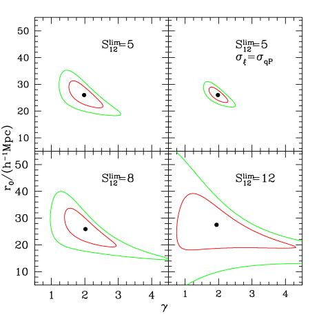
Figure 3: Iso–$\Delta\chi^{2}$ contours on the $r_{0}$–$\gamma$ parameter space from the correlation analysis of samples (a), (b) and (c) (upper left, lower left and lower right panels, respectively). The upper right panel show the results for sample (a) if quasi–Poissonian errors for $\xi(r)$ were instead assumed. Contours correspond to $1\sigma$, $2\sigma$ and $3\sigma$ confidence levels for 2 significant fitting parameters.

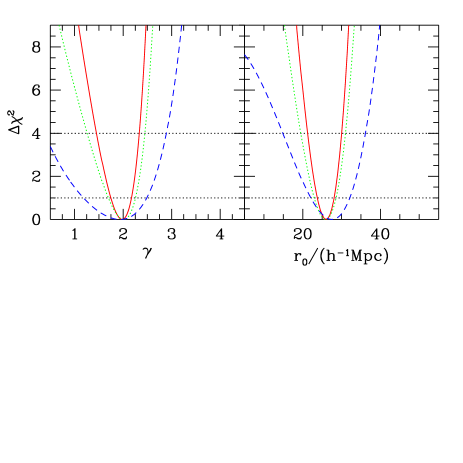
Figure 4: The variation of $\Delta\chi^{2}$ around the best–fitting value of each parameter, after marginalising with respect to the other parameter. Continuous, dotted and dashed curves are for (a), (b) and (c) samples, respectively. The two horizontal lines and the upper limit of each panel represent the $1\sigma$, 2$\sigma$ and 3$\sigma$ confidence levels for one significant parameter.

The biasing factor, $b(M,z)$, appearing in eq.(6) is given by

$$b(M,z)\,=\,1+{[\delta_{c}(z)/\sigma(R_{M},z)]^{2}-1\over\delta_{c}(z)}$$ (8)

(e.g, MW; Matarrese et al. 1997; Baugh et al. 1998). Here $\delta_{c}(z)$ is the critical linear overdensity for spherical collapse. For a critical–density Universe $\delta_{c}=1.686$, independent of $z$, with a weak dependence of the geometry of the Friedmann background (e.g., Eke, Cole & Frenk 1996). Furthermore,

$$\sigma^{2}(R_{M},z)\,=\,\left[{D(z)\over D(0)}\right]^{2}{1\over 2\pi^{2}}\,\int_{0}^{\infty}dk\,k^{2}\,P(k)\,W^{2}(kR_{M})\,.$$ (9)

is the fluctuation variance at mass $M$ and redshift $z$, with $W(x)$ the Fourier representation of the window function, which describes the shape of the volume from where the collapsing object accreates matter. The comoving fluctuation size $R_{M}$ represents the Lagrangian cluster radius. It is connected to the mass scale $M$ and to the present day average matter density $\bar{\rho}$ according to

$$R_{M}\,=\,\left({3M\over 4\pi\bar{\rho}}\right)^{1/3}$$ (10)

for the top–hat window, $W(x)=3(\sin x-x\cos x)/x^{3}$, that we adopt in the following.

Since in practical cases one is interested in the correlation of halos with mass above a given limit $M$, the biasing factor in eq.(8) should be replaced by an effective bias, $b_{eff}$, whose value is obtained by averaging $b$ over the mass distribution of the virialized halos:

$$b_{eff}(M,z)\,=\,{\int_{M}^{\infty}dM^{\prime}\,b(M^{\prime},z)\,n(M^{\prime},z)\over\int_{M}^{\infty}dM^{\prime}\,n(M^{\prime},z)}\,.$$ (11)

In the above expression the mass distribution $n(M,z)$ is given by the Press & Schechter (1974) expression

$$n(M,z)\,dM\,=\,\sqrt{2\over\pi}\,{\bar{\rho}\over M^{2}}\,{\delta_{c}(z)\over\sigma(M,z)}\,\left|{d\log\sigma(M,z)\over d\log M}\right|\,$$

$$\exp\left(-{\delta_{c}^{2}(z)\over 2\sigma^{2}(M,z)}\right)\,dM\,.$$ (12)

The power–spectrum $P(k)$ of density fluctuations can be expressed as $P(k)=Ak^{n}T^{2}(k)$, where $n$ is the primordial spectral index. A Harrison-Zel’dovich primordial spectrum, with $n=1$, will be assumed in the following. As for the transfer function, $T(k)$, we take the expression

$$T(q)\,=\,{{\rm ln}(1+2.34q)\over 2.34q}\times$$

$$\left[1+3.89q+(16.1q)^{2}+(5.46q)^{3}+(6.71q)^{4}\right]^{-1/4}\,.$$ (13)

Here $q=k/h\Gamma$, $\Gamma$ being the shape parameter. For the class of CDM models, it is $\Gamma\simeq\Omega_{0}h$ (Bardeen et al. 1986), while in general $\Gamma$ can be viewed as a free parameter, to be fitted against observational constraints. For instance, the power–spectrum of APM galaxies provide $\Gamma=0.23\pm 0.04$ (e.g., Peacock & Dodds 1996). As for the amplitude of $P(k)$, it is customary to express it in terms of $\sigma_{8}$, the r.m.s. fluctuation amplitude within a top–hat sphere of 8 $h^{-1}{\mathrm{Mpc}}~{}$radius.

Therefore, each model for large–scale structure formation will be characterised by three parameters, namely $\Omega_{0},\sigma_{8}$ and $\Gamma$. In the following, we will present results on the $\Gamma$–$\sigma_{8}$ plane, fixing the density parameter to either $\Omega_{0}=0.3$ or $\Omega_{0}=1$.

The reliability of the MW approach to describe the clustering of cluster–sized halos has been already tested by Mo, Jing & White (1996; cf. also Governato et al. 1998). Jing (1998) recently showed that a correction to eq.(8) is required only for halos of mass much smaller than $M^{*}$ (defined as the mass for which $\delta_{c}/\sigma_{M}=1$), a regime which is not relevant for clusters in plausible cosmological models. Colberg et al. (1998) found from the analysis of their Hubble Volume Simulations that the MW method overpredicts the cluster correlation length $r_{0}$ by $\sim 20\%$. In the following analysis we will compute the biasing factor according to eq.(11) by assuming for $\delta_{c}$ the canonical value of the spherical top–hat collapse model. We just point out that, since $b_{eff}$ depends on $\delta_{c}$ and $\sigma_{M}$ only through their ratio, a change in the choice of $\delta_{c}$ turns into a proportional change in the resulting values of $\sigma_{8}$.

Finally, since the real data are analysed in redshift space, we introduce the effect of $z$–distortion in the MW expression for $\xi(r)$. Redshift–space correlations are amplified by the usual factor $K(\beta)=1+2\beta/3+\beta^{2}/5$ (Kaiser 1987), where $\beta\simeq\Omega_{0}^{0.6}/b_{eff}$. However, for the cluster case where $\beta\sim 0.20$, the effect is rather small since it increases $\xi(r)$ by only $\sim 15\%$.

3.2 Converting fluxes into masses

Cluster masses are the input quantities for the MW analytical approach that we have just described. Since the observable quantity is the cluster luminosity rather than its mass we should provide a suitable method to convert mass into fluxes (or vice-versa).

As a first step we convert masses into $X$–ray temperatures. According to the spherical collapse model and under the assumption of virial equilibrium, the mass–temperature relation can be written as

$$k_{B}T = {1.38\over\beta_{T}}\,\left({M\over 10^{15}h^{-1}M_{\odot}}\right)^{2/3}$$ (14)

$$\times \left[\Omega_{0}\Delta_{vir}(z)\right]^{1/3}(1+z){\rm keV}\,,$$

where 76% of the gas is assumed to be hydrogen (see, e.g., Eke et al. 1996). $\Delta_{vir}(z)$ is given by the ratio between the mean density within the virialized region and the average cosmic density at redshift $z$. For $\Omega_{0}=1$ it is $\Delta_{vir}=18\pi^{2}$, independent of $z$, while we use the expressions provided by Kitayama & Suto (1996) for the $\Omega_{0}=0.3$ cases. For isothermal gas, the $\beta_{T}$ parameter is defined as the ratio of the specific kinetic energy of the collisionless matter to the specific thermal energy of the gas, $\beta_{T}={\mu m_{p}\sigma_{v}^{2}\over k_{B}T}$, with $\mu=0.59$ the mean molecular weight, $m_{p}$ the proton mass and $\sigma_{v}$ the one–dimensional cluster internal velocity dispersion. Equivalence between specific gas thermal energy and DM kinetic energy implies $\beta_{T}=1$. However, neither of such assumptions may be completely correct.

The calibration of the $\beta_{T}$ value using numerical simulations has been attempted by several authors (see, e.g., Bryan & Norman 1998, for a summary of numerical results). Recent simulations of the Santa Barbara Cluster Comparison Project (Frenk et al. 1998), based on a variety of numerical techniques, indicate that $\beta_{T}\simeq 1.15$. This value will be adopted in the following as the fiducial one, while we will also show the effect of changing this parameter over a rather broad range. For instance, a smaller $\beta_{T}$ gives a smaller mass and, therefore, a larger $\sigma_{M}$, at a fixed temperature, so as to reduce the biasing factor in eq.(11). One should however bear in mind that such N–body calibrations of $\beta_{T}$ generally include only adiabatic physics of the intra–cluster medium, while neglecting the effects of radiative cooling, feedback effects from galactic winds, etc.

As a second step we convert $X$–ray temperatures into bolometric luminosities, $L_{bol}$. This is probably the most delicate step of our procedure, since neither observations nor theoretical modelling converge to a unique, well determined $L_{bol}$–$T$ relation. By adopting a phenomenological approach, we model the $L_{bol}$–$T$ relation as

$$L_{bol}\,=\,L_{6}\,\left(T\over 6{\rm keV}\right)^{\alpha}(1+z)^{A}\times 10^{44}h^{-2}\,{\rm erg\,s^{-1}}\,\,,$$ (15)

where $L_{6}$ gives the expected luminosity for a 6 keV cluster, while $A$ defines the redshift evolution of the $L_{bol}$–$T$ relation. Data for local clusters indicates that $L_{6}\simeq 3$ as a rather stable result, and $\alpha\simeq 2.5$–3.5, at least for temperatures $T\raise-2.0pt\hbox{\hbox to0.0pt{\hbox{$\sim$}\hss}\raise 5.0pt\hbox{$>$}\ }1$ keV, depending on the sample, data analysis technique and corrections for cooling flow effects. White, Jones & Forman (1997) analysed a set of 207 EINSTEIN clusters and found $\alpha\simeq 3$, thus in agreement with previous results (e.g., David et al. 1993, and references therein). Although the formal fitting uncertainties are generally small, the scatter of data points around the relation (15) is so large as to raise the question of whether it represents a good model for the observational $L_{bol}$–$T$ relation. A remarkable reduction of the scatter is found once the effects of cooling flow are properly introduced, at least for temperatures $k_{B}T\raise-2.0pt\hbox{\hbox to0.0pt{\hbox{$\sim$}\hss}\raise 5.0pt\hbox{$>$}\ }4\,$keV (e.g., White et al. 1997; Arnaud & Evrard 1997; Markevitch 1998; Allen & Fabian 1998). In the following we will adopt the value $\alpha=3$ as the reference one, while we will also show the effect of its variation on the resulting model constraints. Since available data of the redshift dependence of the $L_{bol}$–$T$ relation indicate no evolution up to $z\simeq 0.4$ (Mushotzky & Scharf 1997) we will use $A=0$ in the following. No dependence of the final results on $A$ are expected, owing to the limited depth of XBACs.

As a third step we convert bolometric luminosities, $L_{bol}$, into finite energy–band ([0.1-2.4] keV) luminosities, $L_{E}$, according to $L_{E}=f_{E}[T(M,z);z]L_{bol}$, where the bolometric correction term, $f_{E}$, is computed by integrating the emissivity over the appropriate energy band. Following Mathiesen & Evrard (1998), we assume in our analysis a purely Bremsstrahlung emissivity, with the power–law approximation for the Gaunt factor, $g(E,T)\propto(E/kT)^{-0.3}$. This approximation has been shown to be rather precise for $T_{X}\raise-2.0pt\hbox{\hbox to0.0pt{\hbox{$\sim$}\hss}\raise 5.0pt\hbox{$>$}\ }2$ keV, which is the temperature range expected to be relevant for the bright Abell clusters of XBACs, in correcting luminosities in the soft ROSAT band, [0.5–2.0] keV (Borgani et al. 1998). We expect this approximation to be at least as good, when dealing with the broader XBACs band.

4 Analysis and results

In order to place constraints on the model parameter space, we should device a method which is able to estimate the values of the slope $\Gamma$ of the power spectrum and its amplitude $\sigma_{8}$, along with the respective statistical uncertainties, in the most assumption–free way.

Binning the data as in Fig. 2 may in principle introduce an uncertainty in the estimated $\xi(r)$, whose value depends in general on the binning choice. Furthermore, the theoretical $\xi(r)$ of eq.(6) requires the value of the mass threshold $M$ to be known. Even for a fixed choice of the mass–luminosity relation, the value of $M$ depends on the effective redshift, $z_{eff}$, that has to be associated to the whole survey. Indeed, for a given flux–limit, the effective luminosity limit is given by

$$L_{eff}\,=\,4\pi d_{L}^{2}(z_{eff})S_{lim}\,,$$ (16)

where $d_{L}$ is the luminosity–distance. In principle, a reasonable choice for $z_{eff}$ is the peak of $N(z)$, which occurs at $\sim 0.075-0.08$ (see Fig. 1). However, due to the broadness of the XBACs redshift distribution, the precise value of $z_{eff}$ can not be fixed in an unambiguous way. We show in Figure 5 the effect of changing the value of $z_{eff}$ from 0.05 to 0.1 on $\xi(r)$, for a fixed cosmological models and $L_{X}$–$T_{X}$ relation. Note that, for both such values of $z_{eff}$, the redshift distribution is far from declining and, therefore, any redshift within this interval can in principle be adopted as $z_{eff}$. Increasing $z_{eff}$ from 0.05 to 0.1, has a non–negligible effect on the resulting $\xi(r)$: the larger $z_{eff}$, the larger the luminosity– and, therefore, the mass–threshold. In turn, this corresponds to a larger biasing factor and, hence, to an increase of $\xi(r)$. Indeed, at $z_{eff}=0.05$, the mass–threshold is $M_{th}\simeq 2.1\times 10^{14}h^{-1}M_{\odot}$ which corresponds to an effective biasing $b_{eff}\simeq 4.6$. Such numbers increases to $M_{th}\simeq 4.4\times 10^{14}h^{-1}M_{\odot}$ and $b_{eff}\simeq 6.2$ for $z_{eff}=0.1$.

This demonstrates that any ambiguity in the choice of $z_{eff}$ generates a similar ambiguity in the determination of the best–fitting model.

Furthermore, at large separations the estimate of $\xi(r)$ is likely to be dominated by more distant and, therefore, more luminous clusters. As a consequence, $\xi(r)$ at different scales takes contributions from cluster populations having different luminosity and, in principle, different clustering properties. A possible solution to this problem would be selecting only clusters above a fixed luminosity limit. It is however clear that this remedy can only be pursued at the expense of substantially reducing the sample statistics.

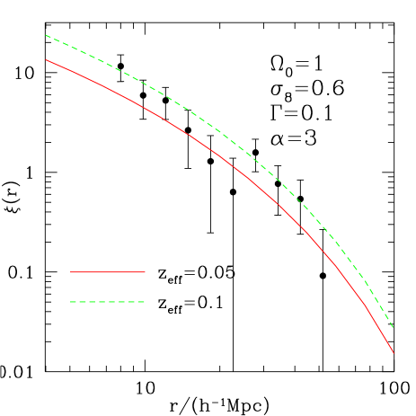
Figure 5: The influence of the choice for the effective survey redshift, $z_{eff}$, on the cluster 2–point correlation function predicted by a specific cosmological model with a fixed $L_{X}$–$T_{X}$ relation. The flux–limit corresponds to that of the sample (a), whose, $\xi(r)$ is also plotted as filled circles.

To overcome such limitations of the binned $\chi^{2}_{min}$ approach, one can estimate the likelihood that the model correlation function produces the measured number of cluster pairs at a given separation and at a given redshift, for specified sample flux–limit and mass–luminosity relation, in a way which does not depend on the binning procedure.

Let $\xi(r,z,M(z))$ be the model correlation function for halos that, at redshift $z$, have mass above the value required by the sample flux–limit. Then, the number of cluster–cluster pairs with separation between $r-dr/2$ and $r+dr/2$ and at redshift between $z-dz/2$ and $z+dz/2$ is

$${\cal C}(r,z)\,dr\,dz\,=\,[1+\xi_{cl}(r,z,M(z))]\,{{\cal R}(r,z)\over 2}\,dr\,dz\,.$$ (17)

Here ${\cal R}(r,z)$ is the expected number of cluster–random pairs, within the same separation and redshift interval. We estimated ${\cal R}(r)$ by averaging over 20,000 random samples. The two–dimensional grid in $r$ and $z$ has 50 equal amplitude bins in the separation interval $6\leq r\leq 56$ $h^{-1}{\mathrm{Mpc}}~{}$and 10 equal amplitude bins for redshift $z\leq 0.2$. It is clear that the bin size can be made as small as desired, by proportionally increasing the number of random samples, so as to make the final results independent of the bin size. The relevant quantity to estimate is the likelihood function ${\cal L}$, which is defined as the product of the probabilities of having one pair at each of the $(r_{i},z_{i})$ bins occupied by the data cluster–cluster pairs and the probability of having zero pairs in all the other elements of the $r$–$z$ plane. By assuming Poisson probabilities for bin occupation, we get

$${\cal L}(r,z) = \prod_{i}\exp[-{\cal C}(r,z)\,dr\,dz]\,{\cal C}(r,z)\,dr\,dz$$ (18)

$$\times \prod_{j\neq i}\exp[-{\cal C}(r,z)\,dr\,dz]\,,$$

where the indices $i$ and $j$ runs over the occupied and empty bins, respectively. The best fitting values of the model parameters are found by minimising the quantity $S=-2{\mbox{\rm ln}}{\cal L}$. After dropping all the terms independent of the cosmological scenario, it reads

$$S\,=\,2\int dr\,\int dz\,{\cal C}(r,z)-2\sum_{i}{\mbox{\rm ln}}{\cal C}(r_{i},z_{i})\,.$$ (19)

A similar maximum–likelihood (ML hereafter) approach has been applied by Croft et al. (1997) to estimate the richness dependence of the correlation length $r_{0}$ of APM clusters (see also Marshall et al. 1983).

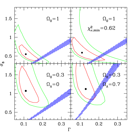
Figure 6: Iso–$\Delta S$ contours on the $\sigma_{8}$–$\Gamma$ plane from the sample (a), for $\Omega_{0}=1$ and 0.3, with both flat and open geometries. The upper right panel show the results from the $\chi^{2}$–minimisation analysis for the critical–density case. Contours correspond to $1\sigma$, $2\sigma$ and $3\sigma$ confidence levels for 2 significant fitting parameters. In each panel, the shaded area represents the 1$\sigma$ confidence region from the COBE normalisation, as given by White & Scott (1997).

The results of the application of the ML analysis are shown in Figure 6, for a low–density model with $\Omega_{0}=0.3$, both with open and flat geometry, and for the critical density case. While the selected range of the shape parameter $\Gamma$ turns out to be almost independent of $\Omega_{0}$, the value of $\sigma_{8}$ is a decreasing function of the density parameter, much like the $\sigma_{8}$ values coming from the local cluster abundance constraint (e.g., Eke et al. 1996; Viana & Liddle 1996; Girardi et al. 1998). It is worth remembering that the confidence regions in the $\sigma_{8}$–$\Gamma$ plane from the ML analysis are estimated with the underlying assumption that cluster pairs are independent of each other. A careful error estimate would pass through the construction of a non–Gaussian likelihood function (e.g., Dodelson, Hui & Jaffe 1997), which in principle requires the knowledge of the whole $N$–point correlation function hierarchy. In their ML analysis of APM clusters, Croft et al. (1998) compared errors from the Poissonian likelihood with the cosmic variance from N–body simulations. They concluded that accuracy of errors from a Poissonian ML function depends on the cluster richness, being rather accurate for cluster populations having a mean separation $d_{cl}\raise-2.0pt\hbox{\hbox to0.0pt{\hbox{$\sim$}\hss}\raise 5.0pt\hbox{$>$}\ }70~{}$ $h^{-1}{\mathrm{Mpc}}~{}$. Assuming $\alpha=3$ in the $L_{X}$–$T_{X}$ relation and $\beta_{T}=1.15$ in the $M$–$T_{X}$ conversion, the XBACs flux–limit corresponds to a cluster mass–limit $\simeq 3.8\times 10^{14}h^{-1}M_{\odot}$ at $z_{eff}=0.08$. In turn, taking the $\Omega_{0}=1$ best–fitting model with $\sigma_{8}=0.55$ and $\Gamma=0.11$, the resulting cluster abundance from the Press–Schechter formula would correspond to $d_{cl}\simeq 85$ $h^{-1}{\mathrm{Mpc}}~{}$for the mean separation of clusters above this mass limit. Therefore, we expect the confidence regions found by the ML approach to provide a realistic estimate of the actual uncertainties in the parameter estimates.

In order to check the robustness of the ML results, we also decided to apply the $\chi^{2}_{min}$ analysis to the binned $\xi(r)$. As already mentioned, a potential limitation of the $\chi^{2}_{min}$ approach lies in the ambiguity in the definition of the effective redshift of the survey. In this analysis, we decided to assume $z_{eff}=0.075$, which corresponds to the peak of the redshift distribution. The results for the $\chi^{2}_{min}$ analysis for $\Omega_{0}=1$ are reported in the upper right right panel of Figure 6. It turns out that the two methods identify essentially the same regions of the $\sigma_{8}$–$\Gamma$ plane. From the one hand, this result supports the robustness of the analysis methods. From the other hand, it indicates that the effective survey redshift is in this case reliably represented by the peak of $N(z)$. We report in Table 2 the best–fitting parameter values, for the three cosmological models, for both the ML and the $\chi^{2}_{min}$ method, along with their 2$\sigma$ uncertainties for one significant parameter, i.e. after maginalising with respect to the other parameter.

We note that $\sigma_{8}$ takes larger values for the smaller $\Omega_{0}$. This is due to the fact that, for fixed cluster distance and flux–mass conversion, the sample flux limit turns into a larger value of the cluster Lagrangian radius $R_{M}$ in eq.(10) when a smaller density parameter is assumed. Therefore, for a fixed $P(k)$ amplitude, clusters would correspond to more rare and thus more clustered peaks. A suitable increase of $\sigma_{8}$ (i.e., of the $P(k)$ amplitude) is thus required to decrease the relative height of the peaks to be associated with clusters.

The resulting constraint on $\sigma_{8}$ and its dependence on $\Omega_{0}$ is comfortably consistent with, although somewhat less stringent than, that coming from the abundance of local galaxy clusters. Indeed, several independent analyses based on the optical virial mass function (e.g., Girardi et al. 1998), the local $X$–ray temperature function (e.g., Viana & Liddle 1996; Eke et al. 1996; Oukbir, Bartlett & Blanchard 1997) and the local $X$–ray luminosity function (e.g., Borgani et al. 1998) converge to indicate that $\sigma_{8}\simeq 0.5$–0.6 for $\Omega_{0}=1$, while it rises to $\sigma_{8}\simeq 0.9$–1.2 for $\Omega_{0}=0.3$, almost independent of the presence of a cosmological constant term. This shows that combining results from cluster abundance and clustering do not allow to break the degeneracy between $\sigma_{8}$ and $\Omega_{0}$. In any case, it is remarkable that both the abundance and the large–scale distribution of clusters, which involve rather different scale ranges, can be consistently interpreted in the framework of hierarchical clustering of Gaussian density fluctuations, as described by the Press & Schechter (1974) approach and by its MW extension to the 2–point correlation function.

As for the shape parameter, it is generally constrained to lie in the range $0.05\raise-2.0pt\hbox{\hbox to0.0pt{\hbox{$\sim$}\hss}\raise 5.0pt\hbox{$<$}\ }\Gamma\raise-2.0pt\hbox{\hbox to0.0pt{\hbox{$\sim$}\hss}\raise 5.0pt\hbox{$<$}\ }0.20$, thus in agreement with, although somewhat smaller than, that obtained from the optical Abell/ACO cluster distribution (Borgani et al. 1997) and from the APM galaxy distribution (e.g., Peacock & Dodds 1994).

The shaded areas in each panel of Fig. 6 represent the 1$\sigma$ constraint from the COBE normalisation, as provided by White & Bunn (1996). It turns out that, if $\Omega_{0}=1$, $\sigma_{8}\simeq 0.4$–0.5 and $\Gamma\simeq 0.18$ (at 1$\sigma$ c.l.) are required to satisfy at the same time the large–scale CMB constraint and the XBACs cluster clustering. As for the low–density flat model, it requires $\sigma_{8}\simeq 0.9$–1.1, with essentially the same shape parameter. As for the open model, CMB and cluster $\xi(r)$ constraints are rather inconsistent with each other.

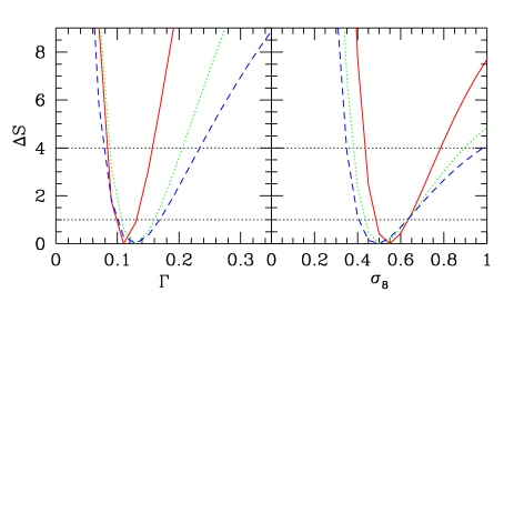
Figure 7: The variation of $\Delta S$ around the best–fitting value of each parameter, after marginalising with respect to the other parameter. Continuous, dotted and dashed curves are for the (a), (b) and (c) samples, respectively. As in Figure 4, the two horizontal lines and the upper limit of each panel represent the $1\sigma$, 2$\sigma$ and 3$\sigma$ confidence levels for one significant parameter.

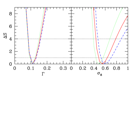
Figure 8: The same as Figure 7, but for the effect of changing the parameter $\alpha$ in the $L_{X}$–$T_{X}$ relation. Dotted, continuous and dashed curves are for $\alpha=2.5,3$ and 3.5, respectively.

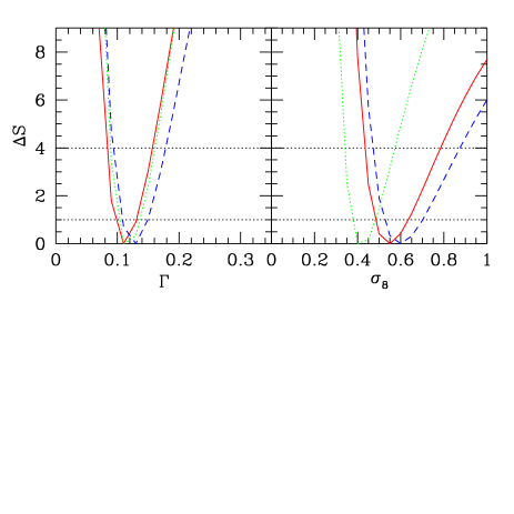
Figure 9: The same as Figure 7, but for the effect of changing the mass–temperature conversion factor, $\beta_{T}$. Dotted, continuous and dashed curves are for $\beta_{T}=0.8,1.15$ and 1.5, respectively.

It is worth reminding here that the above results refer to the whole XBACs, with $S_{\rm lim}=5\times 10^{-12}\,$erg s${}^{-1}\,$cm^-2, as well as to one particular choice of the $L_{X}$–$T_{X}$ relation and of the $M$–$T_{X}$ conversion factor $\beta_{T}$.

In Figure 7 we plot for the $\Omega_{0}=1$ case the variation of $\Delta S=S-S_{min}$ around its minimum, as one of the two parameters $\sigma_{8}$ and $\Gamma$ is varied, keeping the other fixed at its best fitting value, for the (a), (b) and (c) samples. It turns out that results are quite stable when varying the flux limit of the XBACs sample analysed; the only significant effect being that of enlarging the confidence intervals as the number of selected clusters decreases with increasing $S_{lim}$. The stability of the results against variations of the flux limit indicates that any possible incompleteness of XBACs at low fluxes has at most a marginal effect.

The effect of changing the shape of the local $L_{X}$–$T_{X}$ relation is shown in Figure 8. The extreme values of $\alpha=2.5$ and 3.5 have been chosen so as to bracket the range of results presented in the literature (cf. the discussion in the previous section). Even in this case, constraints on model parameters are rather robust against changes in the $L_{X}$–$T_{X}$ relation. This represents a remarkable result, since connecting luminosities to temperatures represents in principle a rather delicate step, owing to the uncertainties in both observational and theoretical determinations of the $L_{X}$–$T_{X}$ relation.

Finally, we show in Figure 9 the effect of changing the parameter $\beta_{T}$ in the $M$–$T_{X}$ relation. Even in this case, the extreme values, $\beta_{T}=0.8$ and 1.5 have been chosen so as to largely encompass the results from hydrodynamic cluster simulations (cf. Bryan & Norman 1998). We find that, while the shape parameter $\Gamma$ does not depend on $\beta_{T}$, the value of $\sigma_{8}$ systematically increases with $\beta_{T}$. The reason for this is that a larger $\beta_{T}$ implies a larger mass for a fixed cluster temperature. As a consequence, a larger $\sigma_{8}$ is required to suppress the biasing factor, so as to compensate for the selection of more massive, more clustered clusters.

Table 2: Model parameters for the sample (a) from the maximum likelihood and from the $\chi^{2}$–minimisation analyses. Uncertainties corresponds to $2\sigma$ confidence levels for one significant parameter.

	Max-like.		$\chi^{2}$–min.
	$\sigma_{8}$	$\Gamma$	$\sigma_{8}$	$\Gamma$
$\Omega_{0}=1$	$0.55^{+0.23}_{-0.11}$	$0.11^{+0.05}_{-0.03}$	$0.59^{+0.30}_{-0.12}$	$0.11^{+0.07}_{-0.04}$
$\Omega_{0}=0.3;\Omega_{\Lambda}=0$	$1.07^{+0.88}_{-0.27}$	$0.11^{+0.06}_{-0.04}$	$1.28^{+0.96}_{-0.26}$	$0.11^{+0.12}_{-0.06}$
$\Omega_{0}=0.3;\Omega_{\Lambda}=0.7$	$1.12^{+0.88}_{-0.29}$	$0.13^{+0.06}_{-0.05}$	$1.50^{+1.33}_{-0.47}$	$0.11^{+0.13}_{-0.06}$

5 Conclusions

We presented an analysis of the redshift–space 2–point correlation function for the X–ray Brightest Abell–type Cluster sample (XBACs; Ebeling et al. 1996), with the aim of investigating the resulting constraints on cosmological models. In our analysis, cosmological models are specified by three parameters, namely the density parameter $\Omega_{0}$ (with or without a cosmological constant term to provide spatial flatness), the fluctuation power–spectrum amplitude through the $\sigma_{8}$ quantity and the shape $\Gamma$ of the power–spectrum.

As a starting point, we follow the analytical approach by Mo & White (1996), which provides the 2–point correlation function, $\xi(r)$, for the distribution of virialized halos above a given mass limit (e.g., Mo, Jing & White 1996). In order to convert masses into observed fluxes, we followed a purely empirical recipe (see also Borgani et al. 1998), which depends on two parameters, namely the conversion factor $\beta_{T}$ to pass from mass to $X$–ray temperatures [cf. eq.(14)] and the slope $\alpha$ of the local $L_{X}$–$T_{X}$ relation [cf. eq.(15)].

Although this analysis is limited to nearby ($z\raise-2.0pt\hbox{\hbox to0.0pt{\hbox{$\sim$}\hss}\raise 5.0pt\hbox{$<$}\ }0.2$) clusters, the formalism that we introduced can be directly applied to any survey of high–redshift objects.

The comparison between model and data has been performed by resorting both to a $\chi^{2}$–minimisation ($\chi^{2}_{min}$) procedure and to a maximum likelihood (ML) approach, which avoids any ambiguity associated to the binning procedure required by the $\chi^{2}_{min}$ method.

The main results of our analysis can be summarised as follows.

(a)

If the 2–point correlation function is modelled as a power–law, $\xi(r)=(r_{0}/r)^{\gamma}$, then the best fitting parameters for the whole sample are $r_{0}=26.0\pm 4.5$ $h^{-1}{\mathrm{Mpc}}~{}$and $\gamma=2.0\pm 0.4$. The clustering strength increases very weakly as a higher flux–limit is imposed and higher luminosity clusters are selected. As long as a correlation exists between cluster luminosity and richness, this result is consistent with the picture of a mild dependence of the correlation amplitude on the cluster richness (cf. Croft et al. 1997).

(b)

For our reference choice for the mass–luminosity conversion (i.e., $\alpha=3$ and $\beta_{T}=1.15$), we find that $\sigma_{8}\simeq 0.6\pm 0.2$ (2$\sigma$ uncertainties after marginalisation), while it becomes about twice as large for $\Omega_{0}=0.3$. This result is completely consistent with constraints coming from cluster abundances and indicates that the picture of hierarchical clustering of Gaussian primordial density fluctuations is able to account at the same time for both the abundance and the clustering of galaxy clusters.

As for the shape of $P(k)$ it is much less dependent on $\Omega_{0}$, with values ranging in the interval $0.05\raise-2.0pt\hbox{\hbox to0.0pt{\hbox{$\sim$}\hss}\raise 5.0pt\hbox{$<$}\ }\Gamma\raise-2.0pt\hbox{\hbox to0.0pt{\hbox{$\sim$}\hss}\raise 5.0pt\hbox{$<$}\ }0.20$. Such results are left unchanged by increasing the sample flux–limit.

(c)

Adding also the large–scale CMB constraints, we find that an $\Omega_{0}=1$ model with $\sigma_{8}\simeq 0.4$–0.5 and $\Gamma\simeq 0.16$–0.20 and a flat $\Omega_{0}=0.3$ model with $\sigma_{8}\simeq 0.9$–1.1 and the same $\Gamma$ are consistent with both the COBE data and the clustering of XBACs clusters. For the open $\Omega_{0}=0.3$ model, the COBE and XBACs constraints are quite inconsistent with each other.

(d)

As for the robustness of such results against changes of the mass–luminosity relation, it turns out that $\Gamma$ is quite insensitive to both the mass–temperature conversion factor $\beta_{T}$ and to the slope $\alpha$ of the local $L_{X}$–$T_{X}$ relation. The power spectrum amplitude $\sigma_{8}$ has only a weak dependence on the choice for the $L_{X}$–$T_{X}$ relation, while it increases from about 0.35 to 0.6 as $\beta_{T}$ varies from 0.8 to 1.5.

As a concluding remark, we point out that, although XBACs provides useful constraints on cosmological models, it is not a completely $X$–ray selected sample. Newer and larger $X$–ray cluster samples have been recently compiled (BCS; Ebeling et al. 1998) or are close to completion (REFLEX; Böhringer et al. 1995). Such samples, thanks to their careful definition of completeness criteria and to their increased statistics will allow to definitely fix the clustering scenario for local $X$–ray clusters. Even more exciting, the possibility of realizing cluster surveys at higher redshifts with next–generation $X$–ray satellites will provide a further means to constrain both the power spectrum of density fluctuations and the value of the matter density parameter.

References

- [] Abadi M.G., Lambas D.G., Muriel H., 1988, ApJ, 507, 526
- [] Abell G.O., 1958, ApJ, 3, 211
- [] Abell G.O., Corwin H.G., Olowin R.P., 1989, ApJS, 70, 1
- [] Allen S.W., Fabian A.C., 1998, MNRAS, 297, L57
- [] Arnaud K.A., Evrard A.E., 1998, MNRAS, submitted, preprint astro–ph/9806353
- [] Bahcall N.A., Soneira R.M., 1983, ApJ, 270, 20
- [] Bahcall N.A., West M., 1992, ApJ, 392, 419
- [] Batuski D.J., Bahcall N.A., Olowin R.P., Burns, J.O., 1989, ApJ, 341, 599
- [] Bardeen J.M., Bond J.R., Kaiser N., Szalay A.S., 1986, ApJ, 304, 15
- [] Baugh C.M., Cole S., Frenk C.S., Lacey C.G., 1998, ApJ, 498, 504
- [] Böhringer H., Guzzo L., et al., 1998, in Proceedings of The 14th IAP Colloquium: Wide Field Surveys in Cosmology (Paris, 1998 May 26-30), eds. S.Colombi, Y.Mellier, p.261
- [] Borgani S., Moscardini L., Plionis M., Górski K.M., Holtzman J., Klypin A., Primack J.P., Smith C.C., 1997, NewA, 1, 321
- [] Borgani S., Rosati P., Tozzi P., Norman C., 1998, ApJ, submitted
- [] Bryan G.L., Norman M.L., 1998, ApJ, 495, 80
- [] Colberg J.M., et al., 1998, in Proceedings of The 14th IAP Colloquium: Wide Field Surveys in Cosmology (Paris, 1998 May 26-30), eds. S.Colombi, Y.Mellier, p.247
- [] Collins C.A., Guzzo L., Nichol R.C., Lumsden S.L., 1995, MNRAS, 274, 1071
- [] Croft R.A.C., Dalton G.B., Efstathiou G., Sutherland W.J., Maddox S.J., 1997, MNRAS, 291, 305
- [] Dalton G.B., Croft R.A.C., Efstathiou G., Sutherland W.J., Maddox S.J., Davis M., 1994, MNRAS, 271, L47
- [] David L.P., Slyz A., Jones C., Forman W., Vrtilek S.D., Arnaud K.A., 1993, ApJ, 412, 479
- [] Dekel A., Blumenthal G.R., Primack J.R., Olivier S., 1989, ApJ, 338, L5
- [] Dodelson S., Hui L., Jaffe A., 1997, preprint astro-ph/9712074
- [] Ebeling H., Voges W., Böhringer H., Edge A.C., Huchra J.P., Briel U.G., 1996, MNRAS, 281, 799
- [] Ebeling H., Edge A.C., Böhringer H., Allen S.W., Crawford C.S., Fabian A.C., Voges W., Huchra J.P., 1998, MNRAS, 301, 881
- [] Eke V.R., Cole S., Frenk C.S., 1996, MNRAS, 282, 263
- [] Frenk C.S., et al., 1998, preprint
- [] Girardi M., Borgani S., Giuricin G., Mardirossian F., Mezzetti M., 1998, ApJ, 506, 45
- [] Governato F., Babul A., Quinn T., Tozzi P., Baugh C.M., Katz N., Lake G., 1998, MNRAS, submitted, preprint astro-ph/9810189
- [] Guzzo L., Böhringer H., et al., 1995, Herstmonceux Conference: Wide–Field Spectroscopy and the Distant Universe, S.J. Maddox & A. Aragon Salamanca eds., Singapore: World Scientific, p.205
- [] Jing Y.P., 1998, ApJ, 503, L9
- [] Jing Y.P., Plionis M., Valdarnini R., 1992, ApJ, 389, 499
- [] Kaiser N., 1987, MNRAS, 227, 1
- [] Kitayama T., Suto Y., 1986, ApJ, 469, 480,
- [] Klypin A., Rhee G., 1994, ApJ, 428, 399
- [] Kolokotronis E., 1998, PhD Thesis, QMW
- [] Markevitch M., 1998, ApJ, 504, 27
- [] Marshall H.L., Avni Y., Tananbaum H., Zamorani G., 1983, ApJ, 269, 35
- [] Matarrese S., Coles P., Lucchin F., Moscardini L., 1996, MNRAS, 286, 115
- [] Mathiesen B., Evrard A.G., 1998, MNRAS, 295, 769
- [] Mo H.J., Jing Y.P., Börner G., 1992, ApJ, 392, 452
- [] Mo H.J., Jing Y.P., White S.D.M., 1996, MNRAS, 282, 1096
- [] Mo H.J., White S.D.M., 1996, MNRAS, 282, 347
- [] Moscardini L., Matarrese S., Lucchin F., Pantano O., Rosati P., 1999, in preparation
- [] Mushotzky R.F., Scharf C.A., 1997, ApJ, 482, L13
- [] Nichol R.C., Briel U.G., Henry J.P., 1994, MNRAS, 267, 771
- [] Oukbir J., Bartlett J.G., Blanchard A., 1997, A&A, 320, 365
- [] Peacock J.A., Dodds S.J., 1994, MNRAS, 267, 1020
- [] Peacock J.A., West M., 1992, MNRAS, 259, 494
- [] Peebles P.J.E., 1993, Physical Cosmology (Princeton: Princeton University Press
- [] Plionis M., Kolokotronis E., 1998, ApJ, 500, 1 (PK98)
- [] Plionis M., Vardarnini R., 1991, MNRAS, 249, 46
- [] Postman M., Spergel D.N., Sutin B., Juszkiewicz R., 1989, ApJ, 346, 588
- [] Press W.H., Schechter P., 1974, ApJ, 187, 425 (PS)
- [] Romer A.K., Collins C.A., Böhringer H., Cruddace R.C., Ebeling H., MacGillawray H.T., Voges W., 1994, Nature, 372, 75
- [] Scaramella R., Zamorani G., Vettolani G., Chincarini G., 1991, AJ, 101, 342
- [] Sutherland W.J., 1988, MNRAS, 234, 159
- [] Trümper J., 1990, Phys. Bl., 46 (5), 137
- [] Viana P.T.P., Liddle A.W., 1996, MNRAS, 281, 323
- [] Voges W., 1992, Proceedings of the Satellite Symposium 3, ESA ISY-3, p.9
- [] White D.A., Jones C., Forman W., 1997, MNRAS, 292, 419
- [] White M., Scott D., 1996, Comm. Ap., 18, 289