The rich cluster of galaxies ABCG 85. IV. Emission line galaxies, luminosity function and dynamical properties.

Abstract

This paper is the fourth of a series dealing with the cluster of galaxies ABCG 85. Using our two extensive photometric and spectroscopic catalogues (with 4232 and 551 galaxies respectively), we discuss here three topics derived from optical data. First, we present the properties of emission line versus non-emission line galaxies, showing that their spatial distributions somewhat differ; emission line galaxies tend to be more concentrated in the south region where groups appear to be falling onto the main cluster, in agreement with the hypothesis (presented in our previous paper) that this infall may create a shock which can heat the X-ray emitting gas and also enhance star formation in galaxies. Then, we analyze the luminosity function in the R band, which shows the presence of a dip similar to that observed in other clusters at comparable absolute magnitudes; this result is interpreted as due to comparable distributions of spirals, ellipticals and dwarfs in these various clusters. Finally, we present the dynamical analysis of the cluster using parametric and non-parametric methods and compare the dynamical mass profiles obtained from the X-ray and optical data.

1 Introduction

As the largest gravitationally bound systems in the Universe, clusters of galaxies have attracted much interest since the pioneering works of Zwicky, who evidenced the existence of dark matter in these objects, and later of Abell (1958), who achieved the first large catalogue of clusters. Clusters of galaxies are now studied through various complementary approaches, e.g. optical imaging and spectroscopy, which allow in particular to derive the distribution and kinematical properties of the cluster galaxies, and to estimate the luminosity function, and X-ray spectral imaging, which gives informations on the physical properties of the X-ray gas embedded in the cluster, and with some hypotheses can lead to estimate the total cluster binding mass.

As a complementary approach to large cluster surveys at small redshifts such as the ESO Nearby Abell Cluster Survey (ENACS, Katgert et al. 1996), we have chosen to analyze in detail a few low-z clusters of galaxies, by combining optical data (imaging and spectroscopy of a large number of galaxies) and X-ray data from the ROSAT archive. We present here complementary results on ABCG 85, which our group has already analyzed under various aspects (see references below).

ABCG 85 has a redshift of z$\sim$0.0555, corresponding to a spatial scale of 97.0 kpc/arcmin (for H${}_{0}=50$ km s^-1Mpc^-1, value that will be used hereafter, together with q₀=0). Its center is defined hereafter as the center of the diffuse X-ray component: $\alpha_{\rm J2000}=$ 0^h41^mn51.9^s, $\delta_{\rm J2000}=$ $-$9^∘18’17” (Pislar et al. 1997). A wealth of data is now available for this cluster: a photometric catalogue of 4232 galaxies obtained by scanning a b_J band photographic plate in a square region $\pm 1^{\circ}$ (5.83 Mpc at the cluster redshift) from the cluster center, calibrated with V and R band CCD imaging taken in the very center (Slezak et al. 1998) and a spectroscopic catalogue of 551 galaxies in a roughly circular region of 1^∘ radius in the direction of ABCG 85, among which 305 belong to the cluster (Durret et al. 1998a). As discussed in our previous papers (Pislar et al. 1997, Lima-Neto et al. 1997, Durret et al. 1998b), there exists in fact a complex of clusters ABCG 85/87/89 in this direction. In X-rays, ABCG 85 shows a homogeneous body, onto which are superimposed various structures: an excess towards the north-west and south-west, a south region superimposed on it, and several blobs forming a long filament towards the south-east; the velocity data confirm the existence of groups and clusters superimposed along the line of sight (see a complete description in Durret et al. 1998b) and show that this X-ray filament seems to be made of blobs falling onto the main cluster.

We present here results on ABCG 85 which may have cosmological implications on the formation of galaxies, clusters and large scale structures. The properties of emission versus non-emission line galaxies will be discussed in section 2 and compared to recent results on emission line galaxies in clusters by Mohr et al. (1996) for ABCG 576 (redshift z=0.038), Biviano et al. (1997) for the large ENACS sample at low redshift (0.035$<$z$<$0.121), and Carlberg et al. (1996) for the CNOC sample at higher redshift (0.1709$<$z$<$0.5466). The cluster luminosity function in the R band will be derived in section 3 and its shape will be compared to that found in other clusters. We will present in section 4 the dynamical properties of the cluster, by estimating the dynamical mass from optical data with various methods and comparing these results with the dynamical mass derived from X-ray data. Finally, conclusions will be drawn in section 5.

2 Comparison of the properties of emission and non-emission line galaxies

In a recent paper based on ENACS data, Biviano et al. (1997, the third paper of the series) gave a good review of the distribution and kinematics of emission line (ELGs) versus non-emission line (NoELGs) galaxies. Their approach is a statistical one, leading to a general picture which fits well in a current scenario of cluster formation. On the other hand, the present study is devoted to a specific cluster, ABCG 85, with already well known general properties; the spirit of this work is therefore closer to that of Mohr et al. (1996).

We will first compare the distributions of ELGs versus No ELGs as a function of various parameters. As pointed out by Mohr et al. (1996), this roughly corresponds to a separation into gas-rich and gas-poor galaxies, with some contamination of the gas-poor sample expected. It can also be considered as a separation into spiral and non-spiral galaxies, with an underestimation of spirals, since not all spirals are ELGs.

The numbers of ELGs and NoELGs in our sample are 102 and 449 respectively. These numbers are reduced to 33 and 272 respectively in the cluster velocity range, defined as the 13000-20000 km s^-1 interval by Durret et al. (1998a). This corresponds to an ELG fraction of 0.11 in the cluster. Such a fraction is in the range derived by Biviano et al. (1997) for the ENACS sample (0.08-0.12), but is notably smaller than the value of 0.34 estimated by Mohr et al. (1996) for ABCG 576.

A classification of the ELGs belonging or not to ABCG 85 based on the equivalent widths of the main emission lines will be performed in a forthcoming paper. The possible existence and influence of environmental effects on the presence and level of activity in galaxies will be discussed in that paper.

2.1 Magnitude distribution

Figure 1: Histogram of the emission line (dashed line), non-emission line (dotted line), and total (full line) numbers of galaxies as a function of magnitude in the R band for all the spectroscopic sample.

Figure 2: Histogram of the emission line (dashed line), non-emission line (dotted line), and total (full line) numbers of galaxies as a function of magnitude in the R band for galaxies in the 13000-20000 km s^-1 velocity range.

Figure 3: Fraction of emission line galaxies as a function of magnitude in the R band for the galaxies with velocities in the 13000-20000 km s^-1 velocity range.

The histograms of the distributions of ELGs, NoELGs and all galaxies as a function of R magnitude are displayed in Fig. 1 for all the galaxies in our redshift catalogue. A similar histogram is drawn in Fig. 2 for galaxies belonging to the 13000-20000 km s^-1 velocity range. NoELGs are seen to be brighter than ELGs in both samples, as in ABCG 576 (Mohr et al. 1996).

The fraction of emission line galaxies (defined in each magnitude bin as the number of emission line galaxies divided by the total number of galaxies) as a function of magnitude in the R band is displayed in Fig. 3 for cluster members. We note an increase of this fraction with magnitude, as expected since for a given exposure time redshifts are easier to obtain for emission line galaxies, which can therefore be measured for fainter objects than for non-emission line galaxies. Note however that this increase becomes steep for R$\geq$17, i.e. even at magnitudes for which there is usually no problem to measure absorption line redshifts, possibly suggesting that ELGs are intrinsically fainter, though it is difficult to ascertain this result since our redshift catalogue is by no means complete in the entire region (its completeness is 85% in a circular 2000 arcsec radius region for R$\leq$18, then drops at larger radii, see Table 2 in Durret et al. 1998a). In order to quantify this effect, we calculated the average luminosities for ELGs and NoELGs in the range 14.5$\leq$R$\leq$17.9. We find average luminosities corresponding to magnitudes of 16.83 and 16.41 for ELGs and NoELGs respectively; the standard errors on the luminosities give corresponding magnitude ranges of [16.65, 17.04] and [16.35, 16.47], which do not overlap. The Kolmogorov-Smirnov and Student tests indeed give probabilities that these two samples originate from the same parent population of 0.0014 and 0.03 respectively, confirming that ELGs are indeed intrinsically fainter that NoELGs. This result is in agreement with that found on a much larger sample by Zucca et al. (1997) of field galaxies.

2.2 Spatial distribution

Figure 4: Fraction of emission line galaxies as a function of projected distance to the cluster center for the galaxies in the 13000-20000 km s^-1 velocity range.

The spatial distributions of ELGs and NoELGs are different for galaxies in the velocity interval 13000-20000 km s^-1. It is generally believed that ELGs are more frequent in the outer regions of the cluster than in the inner zones (Biviano et al. 1997, Fisher et al. 1998). This result is indeed confirmed here in ABCG 85. Fig. 4 shows the fraction of emission line galaxies (estimated as the ratio of the number of emission line galaxies to the total number of galaxies in concentric rings 500 arcsec wide around the cluster center) as a function of projected distance to the cluster center for the galaxies in the 13000-20000 km s^-1  velocity range. This fraction increases towards the outer regions of the cluster, implying a difference in the spatial distributions of ELGs and NoELGs.

Figure 5: Adaptive kernel map of the spatial density distribution of non-emission line galaxies. The axes are the positions relative to the cluster center (defined in the text) in arcseconds. North is to the top and east to the left.

Figure 6: Adaptive kernel map of the spatial density distribution of emission line galaxies. The axes are the positions relative to the cluster center (defined in the text) in arcseconds. North is to the top and east to the left.

In order to visualize better the spatial distributions of both kinds of galaxies, we have drawn adaptive kernel maps (e.g. Pisani 1993) of the spatial density distributions of ELGs and NoELGs; these are shown in Figs. 5 and 6 for all galaxies in the spectroscopic sample, disregarding their velocities. The distribution of NoELGs (Fig. 5) is comparable to that derived from our much larger photometric catalogue for all galaxies, independently of spectral features and cluster membership (see Fig. 1 in Slezak et al. 1998): it is elongated along PA$\sim 160^{\circ}$ and shows a strong concentration around ABCG 85, a secondary peak towards the south east coinciding with ABCG 87 (see for example Table 2 in Durret et al. 1998b) and an enhancement roughly at the position of ABCG 89 to the north west (as discussed by Durret et al. 1998b). The galaxy distribution of ELGs (Fig. 6) is quite different: its peak does not coincide with ABCG 85, but is close to the position of ABCG 87; it shows a weak secondary maximum in the north-northeast direction and elongations along several PAs, all quite different from 160^∘.

2.3 Velocity distribution

Figure 7: Histogram (dashed line) and wavelet reconstructed density distribution (full line) of the velocity of non-emission line galaxies in the [13000-20000 km/s] interval.

Figure 8: Histogram (dashed line) and wavelet reconstructed density distribution (full line) of the velocity of emission line galaxies in the [13000-20000 km/s] interval.

The mean and median velocities, as well as the velocity dispersions are quite different for ELGs and NoELGs; the mean velocities are 15968 and 16627 km s^-1, the median velocities are 15701 and 16732 km s^-1, and the velocity dispersions are 1606 km s^-1  and 1109 km s^-1  for ELGs and NoELGs respectively, suggesting that the morphology-density relation is coupled with kinematic differences. Biviano et al. (1997) found differences in the average velocities of ELGs and NoELGs at a level larger than 2$\sigma$ only for 12 clusters out of their sample of 57; their interpretation was that in these 12 clusters ELGs are a non-virialized population falling onto the main cluster. In a much smaller sample of 6 clusters, Zabludoff & Franx (1993) also found a difference in mean velocity between spirals and early type galaxies in 3 clusters; on the other hand, Mohr et al. (1996) found that in ABCG 576 ELGs and NoELGs had the same average velocity, but with ELGs having a larger velocity dispersion, as in ABCG 85.

The velocity distributions displayed in Figs. 7 and 8 were obtained simultaneously using profile reconstructions based on a wavelet technique and classical histograms. We remind the reader that the features obtained with the wavelet method are significant at a 3$\sigma$ level above the noise (estimated at the smallest scale, see Fadda et al. 1998). While the velocity distribution of NoELGs shows only one peak around 16800 km s^-1 close to the mean or median previously given, that of ELGs shows a peak at about 15300 km s^-1 and a much smaller one around 19250 km s^-1. Therefore, calculations of a mean value and of a velocity dispersion for the total sample of ELGs in ABCG 85 do not characterize the ELG velocity distribution properly. The mean (median) velocity for galaxies belonging to the main ELG component (corresponding to v$<$18000 km s^-1) is 15394 km s^-1 (15411 km s^-1) and the velocity dispersion is 900$\pm$190 km s^-1, much smaller than the value of 1606 km s^-1 previously calculated. The second small peak includes five galaxies, and has a mean (median) value of 19170 km s^-1(19320 km s^-1) and a velocity dispersion of 320 km s^-1. Three of these five galaxies are very close both spatially and in velocity space, suggesting that they are part of a physical group. Notice that the velocity distribution of NoELGs is not gaussian. A more detailed velocity analysis of the total sample of galaxies can be found in Durret et al. (1998b).

Furthermore, it is interesting to note that the minimum of ELG velocity density is obtained for $\simeq 17800$ km s^-1 close to the maximum for NoELG velocity density ($\simeq 17000$ km s^-1); the two samples are therefore different in velocity space, as confirmed by statistical tests (see Table 1 and section 2.4).

The fraction of ELGs seems to increase with velocity. It is about 0.12 within the cluster velocity range, and increases to 0.25-0.33 for background objects (those with velocities larger than 20000 km s^-1), with an extreme value of 0.45 in the last velocity bin (velocities larger than 60000 km s^-1). Such variations are obviously at least partly due to a selection effect (the redshifts of faint background galaxies are easier to measure for emission line than for absorption line spectra), but are difficult to interpret because of the incompleteness of our velocity catalogue at large radial distances.

2.4 Are the ELG and NoELG properties significantly different?

As shown above, the spatial, magnitude and velocity distributions of ELGs and NoELGs are different. In order to quantify statistically these results, we have tested the null hypothesis which would assume both samples to be issued from the same parent population, both in velocity space (v) and spatially (right ascension $\alpha$, declination $\delta$ and projected distance to the cluster center D).

The statistical tests used are the unpaired comparison t-test and the Kolmogorov-Smirnov (K.-S.) test. The former is based on the comparison of the means of both samples (ELGs and NoELGs). Since we have seen that the velocity distribution of ELGs is bimodal, we have applied this test in two velocity ranges: (A) [13000-20000 km/s], corresponding to the entire cluster velocity range, and (B) [13000-18000 km/s], where the second small peak in velocity distribution of the ELGs is eliminated, while the NoELG distribution is not strongly affected.

Table 1: Statistical tests on the properties of ELGs and NoELGs

Probability of	v	$\alpha$	$\delta$	D
Null hypothesis
Student (A)	0.0074
Student (B)	$<0.0001$
K.-S. (B)	0.0004	0.77	0.0490	0.0066

The results are shown in Table 1, indicating that the null hypothesis is rejected with a high degree of confidence. This result is confirmed by the non-parametric K.-S. test, which was applied to the four characteristic properties of both samples. Except for the $\alpha$ variable, all the other quantities give weak probabilities for the null hypothesis.

2.5 Physical interpretation

We have previously shown (Durret et al. 1998b) that ABCG 87 is made of several small groups falling onto the main body of ABCG 85. This picture also allows us to give a general explanation of the ELG properties described above. The density-morphology relation (e.g. Adami et al. 1998a and references therein) shows that the less dense a region, the larger the rate of late type galaxies. Spirals, and consequently ELGs (which are mainly spirals) would therefore tend to avoid the central region of ABCG 85. Since groups of galaxies are less dense, spirals tend to be more numerous in the ABCG 87 region (both in space and in velocity space, see sections 2.2 and 2.3). Moreover, the arrival of these groups onto ABCG 85 probably creates shocks, which leads the temperature of the X-ray emitting gas to increase, as indeed observed in the ASCA temperature map obtained by Markevitch et al. (1998). The shocks induced by the merging of groups into the main cluster may well trigger star formation in gas-rich spiral galaxies and account for the increase in the number of ELGs in the ABCG 87 region (assuming that the general identification of spirals with ELGs is valid). Such a picture is consistent with numerical simulations (e.g. Bekki 1998), in which merging phenomena in clusters trigger star formation, and therefore enhance the numbers of ELGs in merging regions.

The velocity dispersion in the main ELG density peak is high (900$\pm 190$ km s^-1). In the general picture described above, the large velocity dispersion found for ELGs can be explained as resulting from the convolution of the velocity dispersion in each blob (typically $\simeq$300 km s^-1) with the velocity of each blob. However, due to the small number of ELGs, it is difficult to show this directly from the ELG data.

In their interesting statistical analysis of the properties of ELGs in nearby clusters based on the ENACS data, Biviano et al. (1997) emphasize some results, in particular the fact that ELGs appear to avoid the central regions of clusters. They propose a schematic model with two types of components, one with a velocity offset relative to the average cluster velocity and a fairly small velocity dispersion, and the other with no velocity offset and a large velocity dispersion.

These properties, combined with others, suggest that ELGs are falling into the central region without having been previously in it. Such a result is also found by Carlberg et al. (1996) for a sample of about 15 clusters with redshifts between 0.17 and 0.55. Notice that the larger velocity dispersion of ELGs compared to NoELGs can at least partly be due to the difficulty of separating various velocity subsamples; it is only in the case of large amounts of data and when the distribution is clearly asymmetric that it is possible to improve the analysis, as in our case. When a particular cluster is studied in detail, one of the two types of components prevails. Infall is generally not spherically symmetric, because it occurs preferably along filaments (van Haarlem & van de Weygaert 1993, West 1994); this is the case in ABCG 85.

3 Luminosity function in the R band

The study of luminosity functions allows to give constraints not only on the cluster galaxy content, such as the relative abundances of the various galaxy types, but also on larger scale properties. In particular, environmental effects have recently been shown to be important in several clusters; in Coma, for example, Lobo et al. (1997) have shown that the faint end of the luminosity function is steeper in the cluster than in the field, except in the regions surrounding the two large central galaxies. This was interpreted as due to the fact that each of these two galaxies is at the center of a group falling on to the main cluster; these groups tend to accrete dwarf galaxies, and as a result the luminosity function is flatter in these regions.

We will discuss here the properties of the bright part of the luminosity function of ABCG 85 in the R band.

3.1 Description of the available samples

In order to estimate the luminosity function, we can use either our redshift catalogue or our CCD imaging catalogue.

The redshift catalogue covers a roughly circular region of 1^∘ radius around the center of ABCG 85; it is the shallowest one: its completeness is 82% for R$\leq$18 in a circle of 2000 arcsec diameter around the cluster center (302 galaxies in this region). We will limit our analysis to this region hereafter.

The CCD imaging catalogue in the V and R bands was obtained from 10 minute exposures in each band, in a small region in the center of the cluster (see Fig. 4 in Durret et al. 1998a), covering an area of 246 arcmin²; 381 and 805 galaxies were detected in the V and R bands respectively.

A photographic plate catalogue (4232 galaxies) has also been obtained by scanning a plate in the b_J band (Slezak et al. 1998). It is complete down to b_J=19.75 in a $2^{\circ}\times 2^{\circ}$ square region; however, since it is shallower than the CCD imaging catalogue, we will not use it here.

Background counts were kindly made available to us in the R band from the Las Campanas survey (LCRS) by H. Lin (see Lin et al. 1996) and from the ESO-Sculptor survey (ESS) by V. de Lapparent and collaborators (see e.g. Arnouts et al. 1997). Note that the LCRS is made in a wide angle and therefore has small error bars in each bin, but is limited to R$\leq$17.8. The ESS is meant to reach very deep magnitudes in a small beam, and therefore its number counts are small at relatively bright magnitudes (for 17$<$R$<$18).

3.2 The R band luminosity function

We have chosen to draw the luminosity function in the R band, because our CCD imaging catalogue is deeper in R than in V. In the bright part (R$\leq$18), we will use galaxies with redshifts in the cluster range, therefore avoiding the problem of background subtraction. For these galaxies, the R magnitude was estimated from the photographic plate b_J magnitude, as explained in Slezak et al. (1998).

Figure 9: Wavelet reconstruction of the galaxy density as a function of absolute R magnitude for galaxies belonging to ABCG 85 with velocities between 13000 and 20000 km/s (full line) and for galaxies in Coma (dashed line). Arbitrary units are used to allow the direct comparison of both distributions.

Fig. 9 shows a wavelet reconstruction of the distribution of galaxies with velocities in the 13000-20000 km s^-1 velocity range as a function of absolute R magnitude (with an adopted distance modulus of 37.6). The wavelet reconstruction shows features significant at a level higher than 3$\sigma$. In the reconstruction process, we are able to use all the available scales actually determined by the number of galaxies in the sample. However, we are not interested by phenomena at very small scales, which anyway are rather noisy. We therefore excluded the two smallest scales in our density profile reconstruction. The resulting density profile shows a dip for R$\simeq 17.1$, which corresponds to an absolute magnitude M${}_{\rm R}\simeq-20.5$.

We also derived the luminosity function from the R CCD imaging catalogue, which is complete to R$\sim$22, or M${}_{\rm R}\sim-15.6$, but in this case it was necessary to subtract a “typical” background contribution in this band. The ESS and the LCRS give consistent number counts for the magnitude bins which they have in common (within poissonian error bars and both normalized to the same area). We constructed a background function as follows: for both surveys, we estimated the numbers of galaxies N_bg per square degree per magnitude bin; we merged both surveys by considering that the background was represented by the LCRS for R$\leq$17.8 and by the ESS for R$>$17.8; we then fit several curves (power laws or polynomials) to the points thus obtained. The best fit was reached for a power law with the following mathematical expression:

$N_{bg}=1.7544\ 10^{-23}\ {\rm R}^{19.758}$

Figure 10: Best fit of the background contribution estimated from the Las Campanas redshift survey for R$<$17.8 and from the ESO-Sculptor survey for R$>$17.8 (see text).

The background counts and fit are displayed in Fig. 10.

Figure 11: Wavelet reconstruction of the number of galaxies per square degree and per magnitude bin as a function of absolute R magnitude for the CCD imaging sample after subtraction of the background contribution (see text). The bottom line indicates the background contribution.

Fig. 11 shows a wavelet reconstruction of the distribution of galaxies derived from our CCD imaging catalogue after subtraction of the background contribution as explained above. The curve has roughly the same shape as that displayed in Fig. 9 for galaxies with redshifts, but it is shifted by $\sim$0.6 magnitude, with a dip now at M${}_{\rm R}\sim-19.9$. As discussed in section 3.4, it was not possible to draw the luminosity function for fainter magnitudes because of the background subtraction problem.

3.3 A dip in the luminosity function?

3.3.1 How real is the dip in the luminosity function?

Figure 12: Top panel: Luminosity function as in Fig. 9 with error bars obtained by a bootstrap technique (see text). Bottom panel: wavelet reconstructions of the luminosity functions at three different scales; error bars are obtained by a Monte-Carlo technique (see text). The dashed line in the bottom panel shows the luminosity function at a scale twice that of the full line.

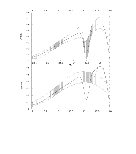
As seen above, the wavelet reconstruction of the galaxy distribution shows a dip. In order to illustrate the robustness of this result, we have done two calculations. First, we consider that our data are the only available realization of a parent sample. Therefore, the bootstrap technique proposed by Efron (1979, 1982) seems well adapted to estimate error bars. We perform 1000 Monte-Carlo draws and do a wavelet analysis on each of the 1000 draws. We choose as limits to the error bars the 10 and 90 percentiles of the distributions thus obtained. These are shown on the top panel of Fig. 12. The dip therefore appears to be statistically significant. However, this bootstrap technique gives too large a weight to the observed realization; in particular, if a gap is present in the data, no draw will be able to fill it.

We have therefore applied a second method. As a first step, we have wavelet reconstructed the luminosity function eliminating the three smallest scales. The distribution obtained in this way does not show any dip. We have then performed 1000 Monte-Carlo draws following this profile, and again have done a wavelet analysis on each of these draws.

The result of this method is shown in Fig. 12 (bottom panel). The dip clearly appears outside the error bar region, implying that the probability to obtain such a feature from such a parent sample (devoid of dips) is smaller than 0.001; even the luminosity function drawn at a larger scale (dashed line in Fig. 12) shows a shallower but still significant dip.

3.3.2 Physical interpretation of the dip

A comparable dip was found in the luminosity function of several clusters. We give in Table 2 the positions of the dips for R band absolute magnitudes recalculated when necessary for a Hubble constant of 50 km s^-1 Mpc^-1; luminosity functions drawn in the B band have been shifted to the R band assuming B$-$R=1.7 for all clusters except Virgo, a typical value for ellipticals, taken as the dominant cluster population. For Virgo, where spirals are dominant, we took B$-$R=1.4. No K-correction or Galactic absorption correction were included, since this is only a rough comparison.

It is interesting to note that the dips in the luminosity functions are found at comparable absolute magnitudes in all these clusters within a range of only one magnitude. The only cluster that we found in the literature having a dip at a significantly different absolute magnitude is ABCG 496.

As mentioned above, the dip position derived from the redshift catalogue differs from that derived from the CCD imaging catalogue in ABCG 85. This apparent discrepancy is most likely accounted for by the fact that the latter corresponds to a much smaller central region, and suggests that environmental effects modify the luminosity function in this cluster (see below).

These dips do not all seem to have the same width: the dip found in the luminosity function of Shapley 8 is notably broader, while shallower dips (or at least flattenings) are found in the luminosity functions of Virgo and ABCG 963. However the methods used by these various authors are quite different from ours; we have redone the analysis described by Biviano et al. (1995) in the Coma cluster using the wavelet reconstruction technique; the corresponding luminosity function is displayed in Fig. 9 and the dip has a shape notably broader than that of ABCG 85.

Table 2: Dip positions in clusters. ABCG 85(z) and (CCD): luminosity functions derived from the reshift and CCD imaging catalogues respectively.

Cluster name	Redshift	Dip position	References
ABCG 85(z)	0.0555	-20.5	This paper
ABCG 85(CCD)	0.0555	-19.9	This paper
ABCG 496	0.0328	-18.0	Molinari et al. (1998)
ABCG 576	0.038	-19.5	Mohr et al. (1996)
ABCG 963	0.206	-19.8	Driver et al. (1994)
Coma	0.0232	-20.5	Biviano et al. (1995)
Shapley 8	0.0482	-19.6	Metcalfe et al. (1994)
Virgo	0.0040	-19.8	Binggeli et al. (1988)

The above facts suggest that the bright galaxy distributions in these clusters have roughly comparable properties, but also that they differ from a cluster to another, and even from one region to another in a given cluster. This is also the case for the relative abundances of galaxy types, which depend on the local density and/or on the global properties of each cluster.

Figure 13: Simulated luminosity function. The bold curve is obtained by the analytical method described in the text. The dashed curve corresponds to the median of Monte-Carlo draws. Error bars are obtained by a Monte-Carlo technique as described previously.

In fact, a simple model based on the shapes of the luminosity functions of the various galaxy types and on their relative proportions (e.g. Böhm & Schmidt 1995, Jerjen & Tammann 1997, and references therein) can roughly account for the dip in the luminosity function.

By using only three kinds of luminosity functions, and adjusting the relative proportions of these three types of galaxies, it is easy to recover a luminosity function with a similar shape to that observed. As an example, such a toy-luminosity function is given in Fig.13; in this case, we have used:

- a Gaussian with $\mu_{R}=$15.8 and $\sigma=$1.1, for the spiral luminosity function;

- a Gamma density (also called Erlang density):

$$G(R)=\frac{\lambda^{\mu}}{\Gamma(\mu)}(R-R_{0})^{\nu-1}\exp-\lambda(R-R_{0})$$

for ellipticals. This density function is asymmetric and has been used by Biviano et al (1995) to describe the luminous part of the Coma luminosity function; $R_{0}$ is a cut-off value (in the example we have chosen $R_{0}=$17.2) the maximum is given by $R_{max}=R_{0}-\frac{\mu-1}{\lambda}$;

- a power law to represent faint or dwarf galaxies, filtered by an apodisation function to account for the incompleteness for high values of R.

We can see from Fig.13 that although located at the good position, the dip is broader than the ABCG 85 dip and not as deep, and that the luminous part of the luminosity function is convex instead of concave. In fact, because the game is played with at least three functions, each of them driven by 3 or even 4 parameters, we have too many degrees of freedom and are able to modify these features in various ways. However, the location of ellipticals relative to dwarfs is well determined: the dip corresponds to the transition zone between ellipticals and dwarfs. However, it has not been possible to play the same game with two functions only.

In this hypothesis, the fact that the dip falls roughly at the same absolute magnitude for at least seven clusters suggests that in the dip region these clusters have comparable galaxy populations; however, the fact that the various dips are not located exactly at the same absolute magnitudes and have different widths raises the question of the relative positions and densities of these various populations. Lobo et al. (1997) have shown that the slope of the faint luminosity function varies with the local environment. The less rich a cluster, the more numerous are spiral galaxies; an increase in the number of spirals will modify the luminosity function only around M${}_{\rm R}\sim-23$. The combination of these well established results leads to confirm, as suggested by previous authors, that in general luminosity functions depend simultaneously on type and on local density and/or global properties (such as cluster richness; see e.g. Phillipps et al. 1998). However, our data is not complete enough to allow a further analysis.

3.4 A word about the faint end of the luminosity function

We initially intended to analyze the faint end of the luminosity function derived from our CCD imaging catalogue after subtracting the background as described above. However, for M${}_{\rm R}>-19.4$ the luminosity function is found to decrease dramatically, rapidly reaching negative values, although the data sample appears to be complete up to R$\sim 22$. This implies that the background contribution has been overestimated, i.e. the “Universal” background counts as obtained in previous section (Fig. 10) are not representative of the background of ABCG 85.

Marginal evidence for the existence of a background larger than expected from statistical arguments has also been found in Coma. Out of 51 redshifts obtained for faint galaxies (R$\leq 21.5$) in a small region near the Coma cluster center, at most five galaxies were found to be cluster members (Adami et al. 1998b), while the expected number was $16\pm 11$. Due to the small number of redshifts involved, this result is of course still preliminary; however, it raises the question of statistical background subtraction, which should not be as universally accepted as it is now.

4 Dynamical analysis

With the assumption that the X-ray emitting gas is isothermal and in hydrostatic equilibrium with dark matter, the dynamical mass was estimated as a function of distance to the cluster center by Pislar et al. (1997) from X-ray (ROSAT PSPC) data (see their Figure 13). Within the X-ray image, which is limited to a distance of 1.3 Mpc around the cluster center, the total mass estimated is about $3\ 10^{14}$ M_⊙.

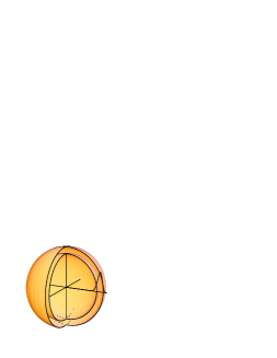
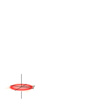
The basic physical picture behind this determination is that if the cluster ABCG 85 is in equilibrium, then the velocities of any subpopulation should reflect the mass distribution. We have calculated the ellipticity of the galaxy distribution using the momentum method. This provided us with a direction of the major axis and the ratio $\epsilon$ of the small to large axes. We have then changed the coordinates of the position of each galaxy by an anamorphosis along the major axis: $X=\epsilon X$. The galaxy distribution then appears spherical. This defines a new radius $R$ which will be used in the following equations. This transformation assumes that the cluster major axis is parallel to the plane of the sky, in the prolate as well as the oblate cases. We may then infer the enclosed mass from the measured velocities of a tracer population. Another possible method which is commonly used is to perform counts in concentric circular rings. Our method is more accurate since the galaxy count estimate is adapted to the geometry, but equation (2) assumes spherical symmetry and is not fully correct. The other method cumulates both defects.

Let us investigate the properties of the cumulative mass profile derived from the different tracers when isotropy is assumed. This is achieved via parametric and non parametric modeling. The Appendix gives a more detailed description of the non-parametric methods involved.

4.1 Data structure

4.1.1 Binning procedure

Optimal inversion techniques should avoid binning while relying on techniques such as Kernel interpolation. We found here that for such a sample and when assessing quantities which are two derivatives away from the data, the Kernel introduces spurious high frequency features in the recovered mass profile. Binning the projected quantities on the other hand allows us to control visually the quality of the fit. We use floating binning which is defined as follows: for each galaxy we find its p-nearest neighbors, and define a ring which encompasses them exactly; the estimator for the density, $\Sigma_{{\mathrm{Ring}}}$, would be defined as p divided by the area of that ring. For the projected velocity dispersion squared, $\sigma_{p}^{2}$, we could sum over the velocity squared (measured with respect to the mean velocity of the cluster) of the p neighbors and divide by p; in practice a better estimator, $\sigma_{p}^{2\star}$, accounting for velocity measurement errors is given by

$$\sigma_{p}^{2\star}=\left(\sum_{i\,\in\,{\mathrm{Ring}}}\frac{v_{i}^{2}}{\sigma_{i}^{2}}\right)\left/\right.\left(\sum_{i\,\in\,{\mathrm{Ring}}}\frac{1}{\sigma_{i}^{2}}\right)\,,$$ (1)

where $\sigma_{i}^{2}$ is the sum of the error on the measured variance, $\sigma_{p}^{2}$, and of the square of the measured error on the velocity $v_{i}$. Bootstrapping is applied to estimate $\sigma_{p}^{2}$ while first neglecting these measurement errors. An estimate of the projected energy density is given by $\sigma_{p}^{2\star}\ \times\Sigma_{{\mathrm{Ring}}}$. In practice, binning over $10$ to $15$ neighboring galaxies is applied, yielding estimates of the Poisson noise induced by sampling.

4.1.2 Bias and incompleteness

The sample is truncated in projected radius $R$. Since generically, truncation and deprojection will not commute, the estimation of the cumulative mass profile arising from a truncated sample in projected radius will be biased. In physical terms, this follows because we cannot distinguish between projected galaxies which are truly within a sphere of radius $R$, and those which are beyond but happen to fall along the line of sight. Considerations about the physical properties of the tracer may help reduce the confusion, but a bias remains in the estimated mass when the sample is truncated in projected radii. Extrapolation provides some means of correction. Note that extrapolation has a different meaning depending on what the true profile is. Specifically the boundary conditions (exponential splines, edge spline, truncation at two or five times the last measured radius) will make a difference in the recovered profile. Since the completeness of our redshift catalogue decreases with increasing radius, we restrict our analysis to the inner region of the cluster within 1000 arcsec (1.62 Mpc at the cluster redshift), where this catalogue is fairly complete (92% for R$\leq 18$). In practice we check that all mass estimates converge to the same total mass within the error bars.

4.2 Method

4.2.1 Jeans equation

The equilibrium of an isotropic stationary spherical galactic cluster obeys Jeans’ equation:

$$M_{dyn}(<r)=r^{2}\frac{{{\mathrm{d}}{\psi}}}{{{\mathrm{d}}{r}}}=-\frac{r^{2}}{\rho}\frac{{{\mathrm{d}}{(\rho\sigma_{r}^{2})}}}{{{\mathrm{d}}{r}}}\,,$$ (2)

where $\psi(r)$ is the gravitational potential generated by all the types of matter, i.e. stellar matter, X-ray emitting plasma and unseen-matter, $\rho(r)$ the density of galaxies in the cluster and $\sigma_{r}(r)$ the radial velocity dispersion. Eq. (2) can be applied locally to assess the cumulative dynamical mass profile.

The surface density of galaxies is related to the density via an Abel transform:

$$\Sigma(R)=\int\limits_{-\infty}^{\infty}\rho(r){{\mathrm{d}}{z}}=2\int_{R}^{\infty}\rho(r)\frac{r{{\mathrm{d}}{r}}}{\sqrt{r^{2}-R^{2}}}\equiv{\cal A}_{R}(\rho)\,,$$ (3)

where $\Sigma(R)$ is the projected galaxy density and $R$ the projected radius as measured on the sky. Similarly the line of sight velocity dispersion $\sigma_{p}^{2}$ is related to the intrinsic radial velocity dispersion, $\sigma_{r}^{2}(r)$, via the same Abel transform (or projection)

$$\Sigma(R)\sigma_{p}^{2}(R)=2\int_{R}^{\infty}\rho(r)\sigma_{r}^{2}(r)\frac{r{{\mathrm{d}}{r}}}{\sqrt{r^{2}-R^{2}}}\equiv{\cal A}_{R}(\rho\sigma_{r}^{2})\,.$$ (4)

Note that $\Sigma(R)\sigma_{p}^{2}$ is the projected kinetic energy density divided by three (corresponding to one degree of freedom) and $\rho(r)\sigma_{r}^{2}$ the kinetic energy density divided by three. Inverting Eqs. (3)-(4) into Eq. (2) yields:

$$M(<r)=-\frac{r^{2}}{{\cal A}^{-1}_{r}(\Sigma)}\frac{{{\mathrm{d}}{{\cal A}^{-1}_{r}(\Sigma\sigma_{p}^{2})}}}{{{\mathrm{d}}{r}}}\,.$$ (5)

Therefore, assuming we have access to estimators for $\Sigma$ and $\Sigma\sigma_{p}^{2}$, the cumulative mass distribution follows.

4.2.2 Algebraic Dynamical Mass estimators

The Bahcall & Tremaine (1981) mass estimator for test particles around a point mass assumes completeness and isotropy and is given by:

$$M(<R_{0})\approx\frac{16}{G\pi}\sum_{i|R_{i}<R_{0}}R_{i}{v_{i}^{2}}\,.$$ (6)

4.3 Parametric modelling

In a nutshell, given that formally the inverse of Eq. (4) is

$$\rho\sigma_{r}^{2}={\cal A}^{-1}_{r}(\Sigma\sigma_{p}^{2})=-\frac{1}{\pi}\int_{r}^{\infty}\frac{{{\mathrm{d}}{}}\Sigma\sigma_{p}^{2}}{dR}\frac{{{\mathrm{d}}{R}}}{\sqrt{R^{2}-r^{2}}}\,{{\mathrm{d}}{R}}\,,$$ (7)

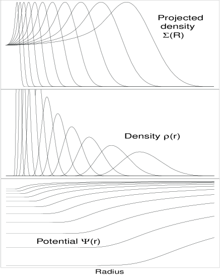
it is straightforward to construct parametric pairs of projected and deprojected fields.

In order to describe the density profile of galaxies, and/or the energy density, we have used various kinds of parametric forms:

1. A $\beta$-model:

   $$\rho(r)=\rho_{0}\left(1+\frac{R^{2}}{b^{2}}\right)^{-3\beta/2}\,,$$ (8)

   for the spatial profile, and

   $$\Sigma(R)=\frac{\rho_{0}b\pi}{\Gamma(3\beta/2)}\left({1+\frac{R^{2}}{b^{2}}}\right)^{(1-3\beta)/2}\Gamma((3\beta-{1})/{2})$$ (9)

   for the projected profile.

2. A Sersic profile

   $$\Sigma(R)={\Sigma_{0}}\,\,{\exp\left({-{{({R\over a})}^{\nu}}}\right)}\,,$$ (10)

   for the projected profile, to which corresponds the spatial profile:

   $$\rho(r)={{{\Sigma_{0}}\,{\Gamma}({2\over{\nu}})}\over{2\,a\,{\Gamma}({{3-p}\over{\nu}})}}{\left({r\over a}\right)^{-p}}{\exp\left({-{{({r\over a})}^{\nu}}}\right)}$$ (11)

   where $p=1-0.6097\nu+0.05463\nu^{2}$ (Gerbal et al. 1997).

3. A power-law for both the spatial and surface energy density since the inverse Abel transform of a power law is a power law with a power index decreased by one.

4.4 Non parametric analysis

The non parametric inversion problem is concerned with finding the best solution to Eq. (5) for the cumulative mass profile when only discretized and noisy measurements of $\Sigma$ and $\Sigma\sigma_{p}^{2}$ are available (Gebhardt et al. 1996, Merritt 1996, Pichon & Thiébaut 1998 and references therein). In order to achieve this goal these functions are written in some fairly general form involving generically many more parameters than constraints and such that each parameter controls only locally the shape of the function. The corresponding inversion problem is known to be ill-conditioned: a small departure in the measured data (due to noise) may produce drastically different solutions since these solutions are dominated by artifacts due to the amplification of noise. Some kind of trade off must therefore be found between the level of smoothness imposed on the solution in order to deal with these artefacts on the one hand, and the level of fluctuations consistent with the amount of information in the signal on the other hand. Finding such a balance is called the “regularization” of the inversion problem.

In practice the regularization can be imposed either directly upon the projected model in data space or upon the unprojected model. The latter (the non parametric inversion) is preferable for Abel transforms such as Eq. (7) since the projection on the sky of a given galaxy distribution is bound to be smoother than the galaxy distribution itself. Moreover, physical constraints such as positivity of the galaxy distribution are also more stringent (and better physically motivated) in model space. Nevertheless it is sometimes more straightforward to carry the regularization in model space (a non parametric fit) and then carry the inversion numerically when an explicit inversion formula such as Eq. (7) is available.

Here, we apply both techniques to the recovery of the mass profile of ABCG 85.

4.4.1 Non parametric fit

We fit a regularized spline to $\log\Sigma$ and $\log\Sigma\sigma_{p}^{2}$ as a function of $\log R$ with a linear penalty function on the second derivative (i.e. which leaves invariant linear functions of $\log_{10}R$ which are power laws of $R$). We then make explicit use of Eq. (7) to compute numerically $\rho$ and $\rho\sigma_{r}^{2}$ together with their derivative. Note that this procedure is a non parametric fit rather than a non parametric inversion, and the regularization parameter needs to be boosted to account for the fact that the fit is then inverted to yield supposedly smooth deprojected quantities. In practice we use the regularization parameter $\mu_{0}=5\mu_{GCV}$ where $\mu_{GCV}$ is given by General Cross Validation as defined in the Appendix.

4.4.2 Non parametric inversion

We fit the projection of a B-spline family which is sampled logarithmically in radius with a linear penalty function on the second derivative as discussed in the Appendix. The coefficients of the fit yield directly $\rho(r)$ and $\rho\sigma_{r}^{2}(r)$ which together with Eq. (2) lead to the cumulative mass profile of ABCG 85. As expected, the error bars on the corresponding mean profile are larger for the non parametric inversion since this method imposes the weakest prejudice on the expected mass profile.

4.5 Results and discussion

We have obtained various dynamical integrated mass profiles, some of which are displayed in Fig. 14, superimposed on those obtained from X-ray data (Pislar et al., 1997). In order to avoid having too many curves on this figure, we omitted the three curves corresponding to the following cases: 2D non parametric fit, galaxy density and pressure following $\beta$–models, and galaxy density following a Sersic distribution and pressure following a $\beta$–model; these three cases are almost indistinguishable from the power law case. Notice that the limiting radius for the mass obtained from optical data (‘optical’ dynamical mass) - 1000 arcsec - is smaller than the limiting radius - 1300 arcsec - for the mass obtained from X-ray data (‘X-ray’ dynamical mass); this is due to the lack of completeness of the galaxy velocity catalogue in a larger region.

Figure 14: Dynamical mass as a function of radius derived with various methods. Full lines: mass derived from X-ray data assuming a $\beta$–model and a Sersic model for the gas distribution; small dotted line: complete non parametric inversion (i.e. 3D model projected in data space); the mean profile and the error bars are estimated while varying the binning from 11 to 18 neighbours; dot-dashed line: galaxy density and pressure following a power law. The large square is the dynamical mass estimated with the Bahcall & Tremaine method.

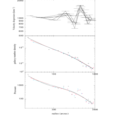
We give in Fig. 15 an example of a non-parametric fit of the observed pressure (bottom panel) and observed profile (middle panel). The observed points for the pressure are the result of the product of the numerical profile with the velocity dispersion shown in the top panel. This profile corresponds to the velocity distribution as a function of projected distance to the cluster center displayed in Fig. 16.

Figure 15: Top panel: velocity dispersion profile ; middle panel: density profile; bottom panel: pressure profile. In the two bottom panels, the observed points are indicated with crosses and typical fits with lines. All these data were obtained with a floating binning mean method. The horizontal lines show the corresponding bins.

Figure 16: Velocity as a function of projected distance to the cluster center for galaxies in the cluster velocity range.

One may notice that the various ‘optical’ dynamical masses are very close to one another, the distances between the curves being smaller than the error bars (see figure); the dynamical mass estimated with the Bahcall & Tremaine method is totally consistent with our estimate.

4.5.1 ‘Optical’ dynamical masses versus ‘X-ray’ dynamical masses

‘Optical’ dynamical masses are larger than ‘X-ray’ dynamical masses. At a distance of R=1000 arcsec, ‘optical’ dynamical masses are $\simeq\leavevmode\nobreak\ 4\leavevmode\nobreak\ 10^{14}$ M_⊙, while ‘X-ray’ dynamical masses are $\simeq\leavevmode\nobreak\ 2\leavevmode\nobreak\ 10^{14}$ M_⊙.

A simple explanation would be the following: from the spectral capability of the ROSAT PSPC, Pislar et al. (1997) have derived an isothermal plasma temperature of about 4 keV. However Markevitch et al. (1998) using ASCA have shown that in the centre of ABCG 85 (where our analysis is performed) the temperature is about 8 keV. Such a discrepancy between ROSAT and ASCA determined temperatures is not uncommon, since the energy range of ROSAT is lower than that of ASCA, and therefore not well suited to measure cluster temperatures. Since ‘X-ray’ dynamical masses are proportional to the temperature, the use of the Markevitch et al. temperature would lead to a dynamical mass $\simeq\leavevmode\nobreak\ 4\leavevmode\nobreak\ 10^{14}$ M_⊙ at R=1000 arcsec, equal to the ‘optical’ dynamical masses. It is then tempting to conclude that the Markevitch et al. high plasma temperature is confirmed by the comparison of ‘optical’ and ‘X-ray’ dynamical masses.

A careful analysis of the ABCG 85 temperature map provided by ASCA (Markevitch et al. 1998) raises the question of the actual gas temperature; the observed value of 8 keV is only valid for a region of about 500 arcsec radius.

Figure 17: ‘X-ray’ dynamical masses estimated in two cases: dotted line: isothermal gas, full line: non-isothermal gas; the error bars are the same as in Fig. 14 for ‘optical’ dynamical masses.

A 3-D temperature profile must be defined by at least three quantities, i.e. a slope (or equivalently an adiabatic index), a length scale and a value of the temperature at a given radius. In the case of ABCG 85, the data are too poor to recover the three above values (Markevitch, private communication). However we have estimated the dynamical mass assuming a “mean” value for the temperature slope compatible with the whole sample of the Markevitch et al. data and using the hydrostatic equation. Notice first that the asymptotic behaviour for the integrated dynamical mass is (obviously) no longer the isothermal one (i.e. $M_{dyn}(r)\propto r^{-\gamma}$, with $\gamma\sim 0.7$). As a consequence the amount of dark matter at large scale would be largely reduced compared to the isothermal behaviour. However, we adress the question of the dynamical mass in a region of only 1000 arcsec. Using a value for the scale length of order 500 kpc we are able to derive a M_dyn profile; the obtained mass compared to the isothermal one is displayed in Fig. 17. As it is the case for some clusters analysed by Markevitch et al. (private communication and poster at the Paris Texas meeting) the non-isothermal mass is higher for small radii but intersects the isothermal profile at a radius of $R_{cut}\sim 800$ arcsec. The resulting profile is clearly located in the region covered with error bars as indicated in Fig. 17.

Our conclusion is that a non-isothermal analysis is not currently possible due to the weakness of the temperature analysis at least for ABCG 85, but is certainly a promising possibility in the future.

One may notice that ‘optical’ dynamical masses show the same rate of growth (i.e. $M(r)\propto r$) as the ‘X-ray’ dynamical masses in the isothermal regime; the corresponding densities vary as $r^{-2}$. We have calculated the 3-D galaxy velocity dispersion profile (defined as the pressure to density ratio). The mean velocity dispersion is 1072 km s^-1 and the residual of this profile compared to this mean value is displayed in Fig. 18; the variation is $\leq 4\%$ indicating that the dispersion profile is constant with radius.

Figure 18: Residual of the deprojected velocity dispersion profile compared to a mean velocity dispersion of 1072 km$s^{-1}$.

Therefore with similar hypotheses - isothermality for the X-ray emitting plasma, isovelocity for the galaxies - ‘X-ray’ dynamical masses and ‘optical’ dynamical masses are equal. This coherence validates the two independent techniques; notice however that the static hypothesis is common for the two methods.

It is interesting to note that the dependence of the mass of the different components with radius (between $\sim$100 and 1000 arcsec) is: $M(r)\propto r^{0.2-0.3}$ for galaxies, $M(r)\propto r^{1.7}$ for the X-ray gas and $M(r)\propto r$ for dynamical matter, as noted above in the isothermal case.

4.5.2 Additional comments

The various modelling techniques implemented onto the masss profile of ABCG 85 have led to very similar featureless powerlaw profiles for the enclosed mass (Fig. 14). This property follows because even with a sample of about 300 galaxies (all the galaxies in the cluster velocity interval were included, i.e. 272 NoELGs and 33 ELGs) the inversion of Eq. (4) or  (3) is dominated by shot noise and requires stringent regularisation. As mentioned previously by Merritt & Tremblay (1994), we find here that a truly non parametric inversion would require that nature provides many more galaxies per cluster.

We remind the reader that we have assumed an isotropic velocity dispersion for the galaxies; the agreement found above shows that this hypothesis is reasonable. It is easily accounted for by the fact that the dominance of radial orbits is probably due to the continuous infall of galaxies and small groups, as shown in particular for ABCG 85 (Durret et al. 1998b), which occurs mostly in the outskirts of the cluster. It is only in the outer regions that the hydrostatic hypothesis is also questionable.

A possible caveat is the following: only the velocity dispersion is observed, while it is the pressure which is the important physical quantity. The estimate of the pressure as the numerical density multiplied by the velocity dispersion is correct if there is no equipartition between small and large galaxy masses, or expressed differently if the velocity dispersion does not depend on the galaxy mass. We have checked in a central region of 750 arcsec radius that the velocity dispersion does not depend on the magnitude; assuming a constant mass to light ratio for all galaxies, this implies that the velocity dispersion does not depend on galaxy mass.

5 Conclusions

The combined large field photographic plate and small field CCD imaging catalogues, coupled with extensive spectroscopic data, have led us to gather one of the largest amounts of data for a single cluster. These data have been used in the present paper to analyze several properties of ABCG 85. Some of these properties have already been discussed in the past by various authors (see Introduction), but the large amount of data now available allows a more refined analysis, leading either to derive new properties or to confirm previous results with a high confidence level.

First, we have compared the distributions of emission line (ELGs) and non-emission line galaxies (NoELGs), and shown that ELGs seem intrinsically fainter than NoELGs, and do not appear as centrally condensed as NoELGs, both spatially and in velocity space. ELGs show an enhancement south of the nucleus, where groups are falling onto the main cluster (as discussed in our previous paper by Durret et al. 1998b). This fits in well with the general view of this cluster: the gas in the galaxies belonging to these groups is expected to be shocked and consequently star formation should be more important in the impact region at the epoch of actual galaxy infall, and less important in the central regions of clusters where star formation appears to be truncated. This has been shown to be the case for two clusters at redshifts 0.2 and 0.4 by Abraham et al. (1996) and Morris et al. (1998). Besides, the cluster analyzed by Abraham et al., ABCG 2390, shows evidence for a subcomponent infalling onto the main cluster, as the south blob is falling onto ABCG 85.

Second, we have analyzed in detail the luminosity function of ABCG 85 in the R band, using a wavelet reconstruction technique. We have shown with a high confidence level that a dip was present at an absolute magnitude M${}_{\rm R}\simeq-20.5$. This feature has also been detected in several other clusters and can be accounted for by the distributions of the various types of galaxies present in the cluster. In this scenario, the dip would correspond to the separation between elliptical and dwarf galaxies.

Third, parametric and non-parametric methods applied to our redshift catalogue have allowed us to derive the dynamical properties of the cluster. We find that the dynamical mass profiles derived from the X-ray gas and galaxy distributions agree if the temperature of the X-ray emitting plasma is about 8 keV. Between 250 and 1000 arcsec, whatever technique we apply (parametric or not), and whatever data we use (X-ray or optical), the slopes of the dynamical mass profiles are the same ($M(r)\propto r$). In this region, both the X-ray plasma and the “gas” of galaxies are isothermal, and the galaxy velocity dispersion is isotropic. If we take into account the temperature gradient of the X-ray gas, the dynamical mass is reduced. If we take into account a possible temperature gradient of the X-ray gas, the ‘X-ray’ dynamical mass is reduced at very large scale but is still comparable to the ‘optical’ dynamical mass in the X-ray emitting region.

Although this paper is the last one of the series on ABCG 85, the analysis of a much larger area in that region of the sky is planned in a near future: we have recently obtained about 300 new redshifts in the direction of ABCG 87 (in collaboration with M. Colless), and have the project of obtaining redshifts for the various clusters and groups aligned along PA$\sim 160^{\circ}$ and in which ABCG 85 seems embedded. We also intend to discuss the large scale structure properties of the universe in the direction of ABCG 85, based on the large scale velocity features of our velocity catalogue.

Appendix A Non parametric analysis

Figure 19: Sketch of deprojection: concentric B-spline shells of increasing logarithmic radii are projected onto the sky; their corresponding light distribution is calculated analytically and represents the basis over which the data is expanded.

Figure 20: The B-spline basis functions and their transform as a function of radius. Top panel: the B-spline projection; middle panel: corresponding density distribution; bottom panel: corresponding self consistent potential.

The non parametric solutions of Eq. (3) and  (4) are described by their projection onto a complete basis of functions

$$\{e_{k}(r)\}_{k=1,\ldots,n}$$

of finite support, which are chosen here to be cubic B-splines (i.e. the unique $C^{2}$ function which is defined to be a cubic over 4 adjacent intervals and zero outside, with the extra property that it integrates to unity over that interval):

$$\rho(r)=\sum_{k=1}^{n}\rho_{k}e_{k}(r),$$ (12)

$$\rho\sigma_{r}^{2}(r)=\sum_{k=1}^{n}(\rho\sigma_{r}^{2})_{k}e_{k}(r)\,.$$ (13)

The parameters to fit are the weights $\rho_{k}$ and $(\rho\sigma_{r}^{2})_{k}$. Calling ${\bf{x}}=\{\rho_{k}\}_{k=1,..n}$ or $\{(\rho\sigma_{r}^{2})_{k}\}_{k=1,..n}$ (the parameters) and $\tilde{{\bf{y}}}=\{\Sigma_{k}\}_{k=1,..K}$ or $\{(\Sigma\sigma_{p}^{2})_{k}\}_{k=1,..K}$ (the measurements) Eq. (3) and  (4) then become formally

$$\tilde{{\bf{y}}}={\bf{a}}\cdot{\bf{x}}\,,$$ (14)

where ${\bf{a}}$ is a $K\times n$ matrix with entries given by

$$a_{i,k}=2\,\int_{R_{i}}^{\infty}e_{k}(r)\frac{r{{\mathrm{d}}{r}}}{\sqrt{r^{2}-R_{i}^{2}}}={\cal A}_{R_{i}}(e_{k})\,.$$ (15)

The projection and the self consistent potential of B-splines can be computed analytically. Their knots can be placed arbitrarily in order to resolve high frequencies in the profiles which are believed to be signal rather than noise (this is a requirement when using a penalty function which operates on the spline coefficient since imposing a correlation between these coefficients would truncate the high frequency). The analytic properties of B-splines and their transform turns out handy in particular since Taylor expansions are available when dealing with exponential profile where the dynamical range is large. Another useful property of B-spline is extrapolation: the correlation of the spline coefficient induced by the penalty function yields an estimate for the behaviour of the profile beyond the last measured point; since the Abel transform requires integration to infinity, this estimate corrects in part for the truncation. Note that an explicit analytic continuation of the model can be added to the spline basis if required. Finally here the requirement is that ${\bf{x}}$ is smooth, which is more strigent than requiring that $\Sigma$ (or $\Sigma\sigma_{p}^{2}$) are smooth.

Assuming that we have access to discrete measurements of $\Sigma$ and $\Sigma\sigma_{p}^{2}$ (via binning as discussed above), and that the noise in $\Sigma$ and $\Sigma\sigma_{p}^{2}$ can be considered to be Normal, we can estimate the error between the measured profiles and the non parametric B-spline model as

$${\mathrm{L}}_{\mathrm{}}({\bf{x}})=\chi^{2}({\bf{x}})={({\tilde{{\bf{y}}}}-{\bf{a}}\!\cdot\!{\bf{x}})^{\bot}}\!\cdot\!{\bf{W}}\!\cdot\!({\tilde{{\bf{y}}}}-{\bf{a}}\!\cdot\!{\bf{x}})\,,$$ (16)

where the weight matrix ${\bf{W}}$ is the inverse of the covariance matrix of the data (which is diagonal for uncorrelated noise with diagonal elements equal to one over the data variance). Linear penalty functions obey

$${\mathrm{R}}_{\mathrm{}}({\bf{x}})={{\bf{x}}^{\bot}}\!\cdot\!{\bf{K}}\!\cdot\!{\bf{x}}\,,$$ (17)

where ${\bf{K}}$ is a positive definite matrix. In practice, we use ${\bf{K}}={{\bf{D}}^{\bot}}\cdot{\bf{D}}$ where ${\bf{D}}$ is a finite difference second order operator

$${\bf{D}}={\rm Diag}_{3}[-1,2,-1]\equiv\left[\begin{array}[]{cccccc}-1&2&-1&0&\ldots&0\\ 0&-1&2&-1&\ldots&\\ &&\ddots&\ddots&\ddots&\\ &&&&&\\ \end{array}\right]\,.$$ (18)

In short, the solution of Eq. (3) (or Eq. (4)) is found by minimizing the quantity $Q({\bf{x}})=L({\bf{x}})+\mu\,R({\bf{x}})$ where $L({\bf{x}})$ and $R({\bf{x}})$ are respectively the likelihood and regularization terms given by Eq. (16) and  (17), ${\bf{x}}$ are the (large number) of parameters, and where the Lagrange multiplier $\mu>0$ allows us to tune the level of regularization. The introduction of the Lagrange multiplier $\mu$ is formally justified by the fact that we want to minimize $Q({\bf{x}})$, subject to the constraint that $L({\bf{x}})$ should be equal to some value. For instance, with $L({\bf{x}})=\chi^{2}({\bf{x}})$ the problem is to minimize $Q({\bf{x}})$ subject to the constraints that $L({\bf{x}})$ is in the range $N_{\mathrm{data}}\pm\sqrt{2\,N_{\mathrm{data}}}$). In practice, the minimum of

$$Q_{\mathrm{}}({\bf{x}})={({\tilde{{\bf{y}}}}-{\bf{a}}\!\cdot\!{\bf{x}})^{\bot}}\!\cdot\!{\bf{W}}\!\cdot\!({\tilde{{\bf{y}}}}-{\bf{a}}\!\cdot\!{\bf{x}})+\mu\,{{\bf{x}}^{\bot}}\!\cdot\!{\bf{K}}\!\cdot\!{\bf{x}}\,$$ (19)

is:

$${\bf{x}}_{\mathrm{}}=({{\bf{a}}^{\bot}}\!\cdot\!{\bf{W}}\!\cdot\!{\bf{a}}+\mu\,{\bf{K}})^{-1}\!\cdot\!{{\bf{a}}^{\bot}}\!\cdot\!{\bf{W}}\!\cdot\!\tilde{{\bf{y}}}\,.$$ (20)

The last remaining issue involves setting the level of regularization. The so-called cross-validation method (Wahba 1990) adjusts the value of $\mu$ so as to minimise residuals between the data and the prediction derived from the data. Let us define

$$\tilde{{\bf{a}}}(\mu)={\bf{a}}\!\cdot\!({{\bf{a}}^{\bot}}\!\cdot\!{\bf{W}}\!\cdot\!{\bf{a}}+\mu\,{\bf{K}})^{-1}\!\cdot\!{{\bf{a}}^{\bot}}\!\cdot\!{\bf{W}}\,.$$ (21)

We make use of the value for $\mu$ given by Generalised Cross Validation (GCV) (Wahba & Wendelberger 1979) estimator corresponding to the mimimum of

$$\mu_{0}\equiv GCV(\mu)={\rm min}_{\mu}\left\{\frac{||({\bf{1}}-\tilde{{\bf{a}}})\!\cdot\!\tilde{{\bf{y}}}||^{2}}{\left[{\rm trace}({\bf{1}}-\tilde{{\bf{a}}})\right]^{2}}\right\}\,.$$ (22)