A Caustic View of Halo Microlensing

Abstract

The only microlensing events towards the Magellanic Clouds for which the location of the lens is strongly constrained are the two binary caustic crossing events. In at least one and possibly both cases, the lens lies at, or close to, the Magellanic Clouds themselves. On the face of it, this seems an improbable occurrence if the Galactic dark halo provides the bulk of the lensing population, as suggested by standard analyses of the MACHO dataset towards the Large Magellanic Cloud (LMC). We use a binomial statistic to assess the prior probability of observing $M$ non-halo binary caustic events given a total sample of $N$ caustic binaries. We generalize for the case of multi-component Galactic and Magellanic Cloud models the Bayesian likelihood method for determining the lens mass and halo fraction from the observed timescales. We introduce a new statistic, the “outcome discriminator”, which measures the consistency between the binary caustic data, prior expectation, and the MACHO two-year LMC dataset as a whole.

If the Magellanic Clouds are not embedded in their own dark halos of MACHOs, then the discovery of two non-halo caustic binary events out of two ($M=N=2$) is inconsistent with expectation given the MACHO dataset. Galactic models in which $M=1$ is the likeliest outcome are also inconsistent with the data, though models in which $M=1$ has a reasonable prior probability are not. We consider the possibilities that the Magellanic Clouds are embedded in dark haloes of their own, or that the Galactic halo is intrinsically deficient in the binary systems which produce caustic crossing events. Either of these possibilities provide greater compatibility between observation and prior expectation, though the idea of Magellanic haloes is perhaps the more natural of the two and has support from kinematical studies.

1 INTRODUCTION

The main motivation driving the microlensing experiments towards the Magellanic Clouds has been the identification of the dark matter content of our Galactic halo. Although there is now no doubt that microlensing events are being detected, their origin is still highly controversial. The sheer number of events seems to argue in favor of the lenses lying in the Galactic halo, but the timescales do not lend themselves to any easy interpretation in terms of known astrophysical objects. This has led a number of investigators to suggest other possible locations for the lenses, including the Magellanic Clouds themselves (Sahu 1994), intervening stellar populations (Zaritsky & Lin 1997), tidal debris (Zhao 1998) or even a warped and flaring Milky Way disk (Evans et al. 1998).

Exotic microlensing, such as parallax and binary events, allow us to break some of the degeneracies in the mass, distance and transverse velocity of the lens (Mao & Paczyński 1991; Gould 1992). In particular, binary caustic crossing events possess a striking lightcurve, enabling unambiguous identification. Even better, the stellar radius crossing time $t_{\star}$ enables the projected transverse velocity $v_{\rm p}=R_{\rm s}/t_{\star}$ at the source to be measured, provided the source radius $R_{\rm s}$ is known. The current follow-up searches of microlensing alerts allow for dense sampling of the lightcurves and permit resolution of the caustic crossing (e.g., Alcock et al. 1997a; Albrow et al. 1998). Thus far, two such binary caustic crossing events have been detected. The first, MACHO LMC-9, had $t_{\star}=0.65$ days and was found by Bennett et al. (1996) for a source star in the Large Magellanic Cloud (LMC). The second and most recent, 98-SMC-1, occurred towards the Small Magellanic Cloud (SMC) and was intensively monitored by three groups (Afonso et al. 1998; Albrow et al 1999; Alcock et al. 1999), who found $t_{\star}=0.12$ days.

Section 2 discusses the likely location of these events. At least one, and possibly both, reside outside of the Galactic halo. Given that halo lenses are expected to outnumber greatly other lens populations, this appears to be a remarkable result. This is confirmed in Section 3, which introduces a binary caustic crossing statistic measuring the prior expectation that $M$ out of a sample of $N$ binary caustic crossing events lie outside of the Galactic halo. Section 4 presents minimal models for the Magellanic Clouds as a prelude to assessing the consistency between prior expectation and observation in Section 5. Here, a new statistic – the “outcome estimator” – is introduced and used to show that there are no minimal models that are consistent with the observed timescales and in which $M=1$ or $2$ is the likeliest outcome, although there are compatible minimal models in which $M=1$ has a reasonable prior probability. Two alternative possibilities – namely that the Magellanic Clouds are swathed in their own dark halos or that the Galactic halo is under-endowed with binaries – are considered in Sections 6 and 7. Finally, we consider the implications of the discovery of further binary caustic crossing events in Section 8.

2 LOCATION OF THE BINARY CAUSTIC EVENTS

For the SMC event, the observed flux and inferred effective temperature of the source suggest that the stellar radius $R_{\rm s}=1.2\,{\rm R}_{\sun}$. Thus, $v_{\rm p}=R_{\rm s}/t_{\star}\simeq 80\,{\rm km}{\rm s}^{-1}$ (Alcock et al. 1999). Recalling that the halo’s optical depth peaks at heliocentric distances of $\sim 10\,{\rm kpc}$, it is easy to calculate that typical halo lenses have $v_{\rm p}\sim 1000\,{\rm km}{\rm s}^{-1}$. The low $v_{\rm p}$ for the SMC event seems to make it certain that the lens responsible does not reside in the Galactic halo but instead belongs to the SMC itself.

The source for the LMC event appears to be a A7-8 main sequence star ($R_{\rm s}\simeq 1.5\,{\rm R}_{\sun}$), in which case $v_{\rm p}\simeq 20\,{\rm km}{\rm s}^{-1}$ (Bennett et al. 1996). Such a value for $v_{\rm p}$ seems unusually low even for LMC lenses. This led Bennett et al. (1996) to suggest that the source itself may be binary, comprising roughly equal luminosity companions with a projected separation $a_{\rm p}$ much less than the projected Einstein radius of the lens $R_{\rm p}$. In such an instance, the crossing time would be given by $t_{*}=a_{\rm p}/v_{\rm p}$. To see how this might affect the inferred location of the binary lens, let us first note from Kepler’s third law that

$$a_{\rm p}\leq a=2.5\,\mbox{AU}\,\left(\frac{P}{10^{3}~{}\mbox{d}}\right)^{2/3}\left(\frac{m_{\rm s}}{{\rm M}_{\sun}}\right)^{1/3}$$ (1)

for a binary system of semi-major axis $a$ and orbital period $P$ comprising stars of equal mass $m_{\rm s}$. The Einstein radius of the lens projected onto the source plane is given by

$$R_{\rm p}=40\,\mbox{AU}\,\left(\frac{m}{{\rm M}_{\sun}}\right)^{1/2}\left(\frac{D}{200~{}\mbox{kpc}}\right)^{1/2},$$ (2)

where $m$ is the lens mass and $D=d_{\rm os}d_{\rm ls}/d_{\rm ol}$, with $d_{\rm os}$, $d_{\rm ls}$ and $d_{\rm ol}$ being the observer–source, lens–source and observer–lens distances, respectively. Fitting to data tabulated in Zombeck (1990), main-sequence sources between $0.4-4~{}{\rm M}_{\sun}$ can be characterized by the following mass–radius relation:

$$R_{\rm s}\simeq\left(\frac{m_{\rm s}}{{\rm M}_{\sun}}\right)^{4/5}{\rm R}_{\sun}.$$ (3)

In order that both binary stars be lensed, we require $a_{\rm p}\ll R_{\rm p}$. Hence, we set $a_{\rm p}<fR_{\rm p}$ ($f\ll 1$). Equations (1), (2) and (3) therefore give the binary semi-major axis in units of stellar radius as

$$\frac{a_{\rm p}}{R_{\rm s}}\lesssim 7\times 10^{3}\,f\left(\frac{m}{{\rm M}_{\sun}}\right)^{1/2}\left(\frac{D}{200~{}\mbox{kpc}}\right)^{1/2}\left(\frac{m_{\rm s}}{{\rm M}_{\sun}}\right)^{-4/5}.$$ (4)

Adopting $f=0.1$, $m=0.5~{}{\rm M}_{\sun}$ and $m_{\rm s}=2~{}{\rm M}_{\sun}$ gives $a_{\rm p}/R_{\rm s}\lesssim 270$. So, whilst taking $v_{\rm p}=R_{\rm s}/t_{\star}$ gives a rather small value of $20\,{\rm km}{\rm s}^{-1}$, if the source is binary one should use $a_{\rm p}$ in place of $R_{\rm s}$, which would make $v_{\rm p}$ up to 2 orders of magnitude larger. This would make it easily compatible with the $v_{\rm p}\sim 1000\,{\rm km}{\rm s}^{-1}$ predicted for halo lenses. Thus, whether the LMC caustic crossing event resides in the halo or not depends crucially on whether the source is binary or not.

What is the likelihood that the source is a binary system with the correct characteristics? The binary fraction is a function of the orbital period $P$. The constraint $a_{\rm p}<fR_{\rm p}$ limits $P$ to

$$P<6.6\times 10^{4}\,{\rm d}\,f^{3/2}\left(\frac{m}{{\rm M}_{\sun}}\right)^{3/4}\left(\frac{D}{200~{}\mbox{kpc}}\right)^{3/4}\left(\frac{m_{\rm s}}{{\rm M}_{\sun}}\right)^{-1/2}.$$ (5)

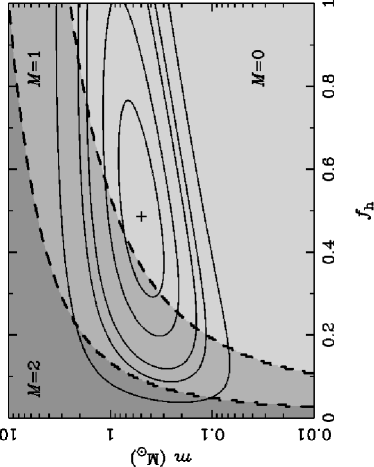
Figure 5: As for figure 3, but with a binary bias $B={\frac{1}{2}}$. This means that the caustic crossing binary fraction is twice as large for the LMC and Milky Way disk than for the Milky Way halo. Again, the “M=1” region shares more of the likelihood than in figure 3.

For the values of $f$, $m$ and $m_{\rm s}$ assumed above, equation (5) gives $P\leq 900$ d. From figure 5 of Abt (1983), A4–F2 stellar systems with periods below 1000 d comprise on average 1.27 members (or 0.27 companions per primary). If this statistic is assumed to be due entirely to single and binary systems, then it implies a binary fraction of $27\%$. Only $39\%$ of A type binaries comprise roughly equal mass stars (Duquennoy & Mayor 1991; Griest & Hu 1992), giving just $10\%$ as the fraction of sources which are binaries with the correct configuration. However, some of the systems tabulated by Abt (1983) comprise more than two members, so in fact this figure is still an upper limit. Assuming these numbers apply to the LMC, then there is no more than a one in ten chance that the crossing time is indicative of the separation between binary companions rather than the size of the stellar disk.

Bennett et al. (1996) put forward the intriguing suggestion of a binary source because they felt that the value of $v_{\rm p}\simeq 20\,{\rm km}{\rm s}^{-1}$ seemed rather low. If the one-dimensional velocity dispersion of the LMC disk is $\sim 25\,{\rm km}{\rm s}^{-1}$ then, as we show in section 4, the most likely value for $v_{\rm p}$ is around $55\,{\rm km}{\rm s}^{-1}$; a velocity as low as $20\,{\rm km}{\rm s}^{-1}$ is only one-tenth as likely. But, this conclusion does depend sensitively on the assumed velocity dispersion. If the velocity dispersion is $\sim 15\,{\rm km}{\rm s}^{-1}$, then the relative probability is more appreciable at $\sim 25\%$ of the peak value. The velocity dispersions of the young, intermediate-age and old stellar populations in such a complex system as the LMC are likely to differ, so it is difficult to judge which value is the most appropriate. We believe that a definite conclusion as to the location of the lens of the LMC binary caustic crossing event cannot be reached with the available evidence. The question could be unambiguously settled by spectroscopy at multiple epochs to see if the source is a radial-velocity variable and hence a binary. Depending on the interpretation of the LMC event, the present observations may be represented by $M=N=2$ or by $M=1,N=2$. Both possibilities are given equal consideration in what follows.

3 BINARIES AND BINOMIALS

Consider a dark Milky Way halo of which some fraction comprises lenses. Of course, there are other populations of lenses along the line of sight to the Clouds – in particular, the Magellanic Clouds themselves and the Milky Way disk. These we collectively refer to as non-halo lenses. Let $R$ (“the rate factor”) be the factor by which the rate of microlensing events caused by halo lenses exceeds the rate of non-halo lenses. In each population, some of the lenses will be binaries, some will not. Only a subset of binaries with particular configurations will give rise to the rather special caustic crossing events. The number of binary caustic crossing events as compared to the total number of all events in each population is unknown, either for the Galactic halo or for non-halo populations. The simplest assumption to make is that this fraction is the same in all components. This may not be the case. First, the fraction of binary stars may vary between stellar populations, second, the distributions of semi-major axes and mass ratios may change according to environment, and third, the caustic-crossing cross section varies with location. Another possibility is a selection bias against events with short intervals between caustic crossings, the majority of which are expected to be caused by halo lenses (Honma 1999). To allow for such effects, let us define $B$ (“the binary bias”) as the ratio of halo to non-halo caustic crossing binary fractions. In other words, if $B=1$, then the fraction of all events that are caustic crossing is the same for all stellar components. If $B={\frac{1}{2}}$, then the non-halo caustic crossing binary fraction is twice as large as that of the halo.

The binomial prior probability of observing $M$ non-halo caustic crossing binaries given a total sample of $N$ such events is then

$${\cal P}(M|N)=\frac{N!}{M!(N-M)!}\left(\frac{1}{BR+1}\right)^{M}\left(\frac{BR}{BR+1}\right)^{N-M}.$$ (6)

The rate factor $R$ contains all the Galactic modeling information, namely the density contribution, velocity distributions and mass functions of the lenses, and also the experimental efficiencies. The two caustic crossing events appeared in different locations (the first towards the LMC, the second towards the SMC) which complicates the computation of $R$. The experimental efficiencies for the SMC observations are not yet available, so it is not possible to assess $R$ along that line of sight. We assume $R$ to be the same along both the LMC and SMC lines of sight. Even if this turns out not to be a good assumption, our results are conservative as long as $R$ towards the SMC is at least as large as $R$ towards the LMC. Since the LMC is substantially more massive than the SMC, this is a reasonable assumption provided that the SMC is not too elongated along the line of sight (see Palanque-Delabrouille et al. 1998). So, if anything, we are overestimating the importance of the Clouds (though see Sahu & Sahu (1998) for a contrary viewpoint).

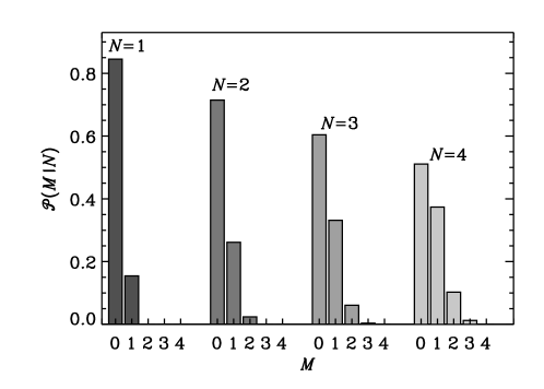
Figure 1: The prior probability of observing $M$ non-halo caustic crossing binaries from a total sample of $N$ such events. The plot assumes a binary bias $B=1$ and a rate factor $R=5.5$. Current observations are best described by $N=2$ and either $M=1$ or 2.

Let us first give an intuitive feel for the meaning of equation (6). Somewhat anticipating the results of the next Section, let us take $R=5.5$. Displayed in figure 1 is the resulting binomial probability ${\cal P}(M|N)$ for $1\leq N\leq 4$ assuming a binary bias $B=1$ (i.e. no bias). We see in figure 1 that for the above parameters ${\cal P}(1|2)$ is $26\%$, whilst ${\cal P}(2|2)$ is very low at $2.4\%$. If the source for the LMC event is indeed binary, thus allowing this event to lie in the halo, then there is nothing remarkable about the present observational status. But, if the source is not binary, then both events are almost certain to be of non-halo origin. In this case, the small prior probability ${\cal P}(2|2)$ does suggest that something is amiss. If a third binary caustic crossing event were to be discovered and found to be non-halo, then the prior probabilities are ${\cal P}(2|3)$ at $6\%$ and ${\cal P}(3|3)$ at just $0.4\%$. Interestingly, only when $N>4$ does the probability of $M>0$ exceed that for $M=0$.

For larger samples (i.e. larger $N$), the probability of any specific outcome ${\cal P}(M|N)$ inevitably decreases because of the increase in the range of possibilities. For this reason, it is preferable to normalize probabilities with respect to the most likely outcome ${\cal P}_{\rm max}(N)$ for a given sample $N$. In the case of $N=2$, the most likely outcome is $M=0$ with ${\cal P}_{\rm max}(2)={\cal P}(0|2)=0.71$ for our assumed $R$. Let us therefore define ${\cal R}(M|N)={\cal P}(M|N)/{\cal P}_{\rm max}(N)$ as the prior relative probability. Thus for $N=2$, ${\cal P}_{\rm max}(2)={\cal P}(0|2)$, so we have ${\cal R}(0|2)=1$, ${\cal R}(1|2)=0.37$ and ${\cal R}(2|2)=0.033$. Even relative to other possible outcomes, two non-halo caustic crossing events from a sample of two is clearly unexpected.

Whilst interesting, these figures are in no sense definitive since they depend on a number of uncertain modeling parameters, which determine the rate factor $R$. The models themselves are of course constrained by the entire microlensing dataset. We therefore undertake a more critical examination by first introducing Galactic and LMC models and then more elaborate statistical techniques in the following two Sections.

4 MINIMAL MAGELLANIC MODELS

The simplest model for the LMC is a bare disk with a central column density of $363\,{\rm M}_{\sun}{\rm pc}^{-2}$ and an inclination angle of $27^{\circ}$ (e.g., Alcock et al. 1996; Westerlund 1997). The mass density of the LMC disk is taken as (c.f., Evans 1996)

$$\rho(R,z)=0.54\exp\left(-0.625\sqrt{R^{2}+28.6z^{2}}\right){\rm M}_{\sun}{\rm pc}^{-3},$$ (7)

where ($R,z$) are the cylindrical coordinates, in kiloparsecs, centered on the LMC. The scale length of the LMC disk is $1.6\,{\rm kpc}$ and the scale height is $300\,{\rm pc}$ (Bessell, Freeman & Wood 1986). The velocity distribution is isotropic and Gaussian with a one-dimensional velocity dispersion of $25\,{\rm km}{\rm s}^{-1}$ about an asymptotic circular velocity of $80\,{\rm km}{\rm s}^{-1}$ (e.g., Schommer et al. 1992; Westerlund 1997). The Galactic halo is represented as an isothermal sphere of core radius $R_{\rm c}=5\,{\rm kpc}$ and an asymptotic circular speed $v_{0}$ of $220\,{\rm km}{\rm s}^{-1}$ (c.f., Griest 1991):

$$\rho(r)={v_{0}^{2}\over 4\pi G(R_{\rm c}^{2}+r^{2})},$$ (8)

where $r$ is a spherical polar coordinate measured from the Galactic Center. The velocity distribution is taken to be isotropic and Gaussian with a dispersion of $155\,{\rm km}{\rm s}^{-1}$. The Galactic disk is modeled by

$$\rho(R,z)=0.62\exp\left(-\frac{R}{3\,\mbox{kpc}}\right){\rm sech}^{2}\left(\frac{z}{0.3\,\mbox{kpc}}\right){\rm M}_{\sun}{\rm pc}^{-3},$$ (9)

where ($R,z$) are cylindrical polar coordinates about the Galactic Center. The column density of the thin disk at the sun is $26\,{\rm M}_{\sun}{\rm pc}^{-2}$, as suggested by Gould, Bahcall & Flynn (1997). The velocities are distributed about the circular speed of $220\,{\rm km}{\rm s}^{-1}$ in Gaussian manner with a dispersion of $30\,{\rm km}{\rm s}^{-1}$. The motion of the line of the sight is taken into account using the proper motion measurement of Jones, Klemola & Lin (1994). The LMC and Milky Way disk lenses are taken to have a fixed mass of $0.35\,{\rm M}_{\sun}$, since this represents the average microlensing mass for a hydrogen-burning population with a Scalo mass function. The Milky Way halo lenses are characterized by a discrete lens mass $m$. With these model assumptions in hand, it is now straightforward to calculate the rate of microlensing.

Figure 2a plots the distribution of projected velocities $P(v_{\rm p})$ for lenses in the Milky Way disk and halo, as well as the LMC disk. (Somewhat anticipating the work in Section 6, the results for an LMC dark halo are also included). Each of the distributions is normalized to have a maximum value of unity. As Bennett et al. (1996) articulate, this is potentially a powerful way to separate the binary caustic crossing events by the location of the lenses. For example, lenses in the Milky Way disk typically lie within heliocentric distances of a kiloparsec, so the projection factor is $\mathrel{\hbox to0.0pt{\lower 3.0pt\hbox{$\sim$}\hss}\raise 2.0pt\hbox{$>$}}50$ and the projected velocities of the lenses $\mathrel{\hbox to0.0pt{\lower 3.0pt\hbox{$\sim$}\hss}\raise 2.0pt\hbox{$>$}}2000\,{\rm km}{\rm s}^{-1}$. The projection factor of lenses in the LMC disk slightly exceeds unity, but the typical projected velocity is $\sim 55\,{\rm km}{\rm s}^{-1}$, a good deal higher than the two-dimensional velocity dispersion. This is because the random velocities of both the lenses and sources contribute and because the event rate is determined by the flux which is velocity weighted. Figure 2b assesses how likely it is that an LMC lens has $v_{\rm p}\simeq 20\,{\rm km}{\rm s}^{-1}$. Here, the relative probability density $P(v_{\rm p}=20)$ is plotted against the velocity dispersion $\sigma$ of the LMC disk. The unbroken line refers to a LMC disk with the standard scale height of $300\,{\rm pc}$, the broken line refers to a super-thin disk with half the standard thickness. Whether such a low $v_{\rm p}$ as $20\,{\rm km}{\rm s}^{-1}$ is likely or unlikely depends sensitively on the assumed velocity dispersion and scale height.

5 THE OUTCOME ESTIMATOR

There are only two free parameters that remain in our model. The first is the lens mass $m$ and the second is the fractional contribution to the halo provided by the lenses, which we denote as $f_{\rm h}$. For a specified Galactic model, both $f_{\rm h}$ and $m$ are constrained by microlensing observations. As ${\cal R}(M|N)$ depends upon these parameters, it too is therefore restricted by the data. Alcock et al. (1997b) use a Bayesian likelihood statistic to constrain both $f_{\rm h}$ and $m$, assuming the observed events all reside in the Galactic halo. We drop this assumption by generalizing their statistic as follows

$$L(f_{\rm h},m|t_{i})=\exp(-f_{\rm h}N_{\rm h}-N_{\rm d})\prod_{i=1}^{N_{\rm obs}}E{\cal E}(t_{i})\left(f_{\rm h}\frac{{\rm d}\Gamma_{\rm h}}{{\rm d}t_{i}}+\frac{{\rm d}\Gamma_{\rm d}}{{\rm d}t_{i}}\right),$$ (10)

where $N_{\rm obs}=8$ is the observed number of events, $E=1.82\times 10^{7}$ star-years is the effective exposure for the Alcock et al. 2-year dataset, ${\cal E}(t_{i})$ is the detection efficiency for events of duration $t_{i}$, $N_{\rm h}$ and $\Gamma_{\rm h}$ are respectively the expected number of events and the event rate for a full halo ($f_{\rm h}=1$), and $N_{\rm d}$ and $\Gamma_{\rm d}$ are the analogous quantities for the combined Milky Way and LMC disk components. Figure 3a plots the resulting likelihood contours (solid lines) in the ($f_{\rm h},m$) plane assuming a uniform prior in $f_{\rm h}$ and logarithmic prior in $m$. The effect of including the non-halo components is that our two dimensional maximum likelihood solution ($f_{\rm h}=0.49,m=0.50\,{\rm M}_{\sun}$, as indicated by the cross) implies a baryonic halo mass inside $50\,{\rm kpc}$ of $2.3\times 10^{11}\,{\rm M}_{\sun}$; this is $80\%$ of the mass derived in the Alcock et al. (1997b) analysis for the same events. Marginalizing over $f_{\rm h}$ gives an allowed range in $m$ of $0.34-1.03\,{\rm M}_{\sun}$ ($0.19-1.82\,{\rm M}_{\sun}$) at the $68\%$ ($95\%$) confidence level. For $f_{\rm h}$, marginalizing over $m$ gives an allowed range of $0.26-0.79$ ($0.12-1.26$).

The shaded regions in figure 3a show the most likely number of non-halo caustic crossing events $M$ given $N=2$ observed binary caustic events. By taking $N=2$, we are including the SMC binary event although the likelihood contours do not incorporate this event. This is justifiable so long as the LMC dataset is truly representative of the halo lens population as a whole. (As we stressed earlier, we are also assuming that the rate factor $R$ is similar along both the LMC and SMC lines of sight). For $(f_{\rm h},m)$ values falling in the darker shaded region to the upper left of the plot, ${\cal R}(2|2)=1$. Thus, the prior expectation is $M=2$ non-halo events (i.e. none of the events reside in the halo) for models in this region. In the lighter shaded region labeled “$M=1$”, ${\cal R}(1|2)=1$, whilst in the lightest shaded region ${\cal R}(0|2)=1$.

At this point it is worth stressing the difference between the model likelihood $L$ and the binary prior relative probability ${\cal R}(M|N)$. A value of ${\cal R}(M|N)$ approaching unity means that $M$ non-halo caustic crossing binaries are consistent with expectation given that $N$ caustic crossing events have been observed. A large $L$ means that the Galactic model (characterized by $m$ and $f_{\rm h}$) is consistent with the timescales $t_{i}$ of all the LMC microlensing candidates. ${\cal R}(M|N)$ is a model dependent quantity, since $f_{\rm h}$ and $m$ are required to calculate ${\cal P}(M|N)$ in equation (6). However, ${\cal R}(M|N)$ does not provide a measure of the likelihood of the underlying model $(f_{\rm h},m)$ itself; it is meaningless to compare values of ${\cal R}(M|N)$ between models with different $(f_{\rm h},m)$ without taking account of the model likelihood $L$ in each case. The likelihood $L$ can be used to assess, in a model independent manner, the relative likelihood of the hypotheses that we inhabit a galaxy in which $M=0$, 1 or 2 is the expected outcome for the case $N=2$. Mathematically speaking, we can use $L$ to test the hypotheses ${\cal R}(0|2)=1$, ${\cal R}(1|2)=1$ or ${\cal R}(2|2)=1$. It is evident from the solid contours that most of the likelihood $L$ is contained within the region where ${\cal R}(0|2)=1$. Integrating the likelihood in each region we find that, given the data, $M=0$ is 40 times more likely to be the expected outcome than $M=1$, and 1700 times more likely than $M=2$.

Whilst we may expect the present observational situation to have a significant prior probability, it would be unreasonable of us to demand that it be the most probable. Since the current caustic binary dataset indicates $N=2$ and $M=1$ or 2, we wish to see whether there are Galactic models that predict significant values for either ${\cal R}(1|2)$ or ${\cal R}(2|2)$ (or both), and which are consistent with the entire dataset (i.e. have a large likelihood $L$). We therefore demand that ${\cal R}(M|N)$ be at least as large as some threshold ${\cal R}_{*}$ where, say, ${\cal R}_{*}=0.1$. In other words, we require the observations to have a prior probability that is at least one-tenth as large as that of the expected outcome. We can again test this hypothesis for each $M$ by integrating the likelihood $L$ over the regions where ${\cal R}(M|N)\geq{\cal R}_{*}$. We therefore wish to compute the “outcome discriminator”

$$D({\cal R}\geq{\cal R}_{*}|t_{i})=\frac{\int\int L(f_{\rm h},m|t_{i})\,\Theta({\cal R}-{\cal R}_{*})\,{\rm d}\ln m\,{\rm d}f_{\rm h}}{\int\int L(f_{\rm h},m|t_{i})\,{\rm d}\ln m\,{\rm d}f_{\rm h}},$$ (11)

where $\Theta$ is the Heaviside step function and uniform priors in $f_{\rm h}$ and $\ln m$ have been assumed. The outcome discriminator is the probability that the condition ${\cal R}\geq{\cal R}_{*}$ holds given the dataset $t_{i}$. Note that, in principle, the cleanest way to interpret the data would be to use a maximum likelihood statistic in $t$ for ordinary events and ($t,v_{\rm p}$) for the binary caustic crossing events. This is not feasible as we would then need to know the theoretical rate and the efficiencies for caustic crossing events towards the Magellanic Clouds.

Figure 3b shows plots of the outcome discriminator $D({\cal R}\geq{\cal R}_{*}|t_{i})$ against threshold ${\cal R}_{*}$ for the case $N=2$. As ${\cal R}_{*}\rightarrow 0$, the outcome discriminator tends to unity because the fraction of the likelihood plane satisfying the threshold ${\cal R}_{*}$ tends to unity. As ${\cal R}_{*}$ increases, the outcome discriminator decreases until, at ${\cal R}_{*}=1$, it attains the limit corresponding to the shaded regions in figure 3a. At first glance the curve for $M=0$ (thick solid line) appears to be insensitive to ${\cal R}_{*}$. Looking back at figure 3a we see that, even when ${\cal R}_{*}=1$, the overwhelming bulk of the likelihood is contained within the $M=0$ region. Therefore, decreasing the threshold ${\cal R}_{*}$ does not significantly increase the value of the outcome discriminator. By contrast, when ${\cal R}_{*}=1$, the $M=1$ and $2$ regions cover very little of the likelihood plane. So, in these cases decreasing the threshold ${\cal R}_{*}$ results in a significant increase in the outcome discriminator. Superimposed on the figure are two cuts, depicted by the hatched regions. The vertical region denotes a minimum acceptable threshold ${\cal R}_{*}=0.1$. Outcomes below this threshold are taken to have unacceptably low prior probability. The horizontal hatched region shows where the condition ${\cal R}\geq{\cal R}_{*}$ has less than $10\%$ chance of being satisfied, given the two-year LMC dataset. It is interesting that with these adopted thresholds, $M=2$ is almost completely excluded: there is no more than a $10\%$ chance that we inhabit a galaxy where ${\cal R}(2|2)$ exceeds 0.1. For $M=1$, models with large prior relative probability (${\cal R}\geq 0.65$) are excluded by the data. This however still leaves viable models in the unhatched region.

Clearly, these figures do not favor the interpretation of both caustic crossing events residing outside the Galactic halo. Therefore, if it really is the case that $M=2$, something must be amiss in our model assumptions. What are our options if this does indeed turn out to be the case?

6 MAXIMAL MAGELLANIC MODELS

If the source stars of the two caustic crossing events really are single, implying that both the lenses are indeed of non-halo origin, then the preceding analysis leads one to think that the Galactic model itself may be wrong. Perhaps the halo is too massive, whilst the LMC disk and Milky Way stellar components are not substantial enough. However, this is not an option because virial arguments preclude the LMC disk from accounting for most of the microlensing events (Gould 1995), whilst the projected velocities of the caustic crossing events are too low to be explained by a Milky Way disk, however massive. Alternatively, there might be an additional dark component which contributes significantly to the microlensing statistics, thereby implying a somewhat reduced Milky Way halo microlensing budget. Natural candidates for this are halos of dark matter enveloping the LMC and SMC themselves – for which there is supporting kinematical evidence (Schommer et al. 1992). Let us therefore immerse the LMC disk in a dark halo using equation (8) with a core radius $R_{\rm c}$ of $1\,{\rm kpc}$, an asymptotic circular speed of $80\,{\rm km}{\rm s}^{-1}$ and velocity dispersion of $55\,{\rm km}{\rm s}^{-1}$. The LMC halo extends to a radius of about $10\,{\rm kpc}$ and – like the Milky Way halo – is assumed to have a fraction $f_{\rm h}$ of lenses of mass $m$. Figure 2 shows the expected distribution of $v_{\rm p}$ for this model, whilst Table 1 summarizes its microlensing properties.

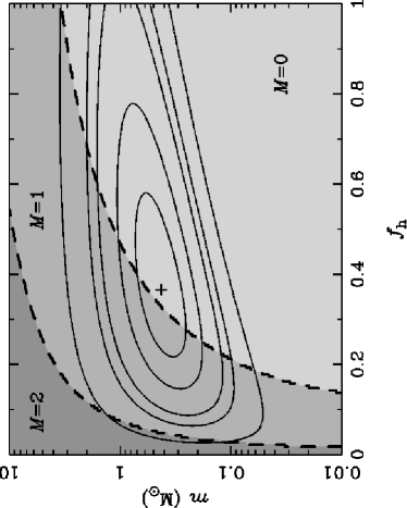
Figure 4: As for figure 3, but for a maximal model in which the LMC possesses a dark halo of its own, characterized by the same baryon fraction $f_{\rm h}$ and lens mass $m$ as the Milky Way halo. Notice that the “M=1” region now occupies a more substantial share of the total likelihood.

The maximum likelihood solution for the combined Milky Way and LMC disk/halo models can be readily evaluated by augmenting the $N_{\rm h}$ and $\Gamma_{\rm h}$ terms in equation (10) with the LMC halo contribution. Figure 4a shows the resulting likelihood contours in the ($f_{\rm h},m$) plane. There is now an additional source of lenses, so the likelihood contours are shifted towards lower values of $f_{\rm h}$. The two dimensional maximum likelihood solution shown by the cross is ($f_{\rm h}=0.37,m=0.43\,{\rm M}_{\sun}$) corresponding to a microlensing halo mass inside $50\,{\rm kpc}$ of $1.7\times 10^{11}\,{\rm M}_{\sun}$. The inclusion of an LMC halo lowers the lens mass $m$ by $18\%$ and the halo mass by $24\%$ relative to the minimal Magellanic model. The marginalized distributions provide the following $68\%$ ($95\%$) limits: $f_{\rm h}$ lies between $0.20-0.61$ ($0.09-0.99$) and $m$ lies between $0.29-0.92\,{\rm M}_{\sun}$ ($0.16-1.79\,{\rm M}_{\sun}$). As in figure 3a, we have shaded the areas of the likelihood plane where $M=0,1$ or 2 is the most probable prior for $N=2$. The most significant change is that the $M=1$ region now occupies a substantial share of the likelihood. Integrating the likelihood in each region we find that, given the data, $M=0$ is twice as likely to be the expected outcome than $M=1$, and 600 times more likely than $M=2$.

Figure 4b shows the outcome discriminator, defined in equation (11), as a function of threshold ${\cal R}_{*}$. We see that $M=0$ and $M=1$ are easily compatible with our adopted cuts. Either of the scenarios are consistent with prior expectation and the observed timescale distribution, though the caustic crossing times of the binary events themselves rule out $M=0$ (see section 2). For thresholds satisfying $0.4\mathrel{\hbox to0.0pt{\lower 3.0pt\hbox{$\sim$}\hss}\raise 2.0pt\hbox{$<$}}{\cal R}_{*}\mathrel{\hbox to0.0pt{\lower 3.0pt\hbox{$\sim$}\hss}\raise 2.0pt\hbox{$<$}}0.7$, the $M=1$ curve lies above the $M=0$ line. This is because the region of the $(f_{\rm h},m)$ plane satisfying these thresholds contains a larger share of the total likelihood for $M=1$ than for $M=0$. However, if we tighten the threshold (i.e., increase ${\cal R}_{*}$), then the likelihood for $M=1$ shrinks faster than for $M=0$. A significant part of the $M=2$ curve now lies in the permitted region in figure 4b, though the observed timescale distribution strongly disfavors models in which $M=2$ is a priori the most probable outcome. Such models represent only $0.1\%$ of the total likelihood. However, there are still models favored by the 2-year LMC dataset in which, although it does not have the largest prior expectation for $N=2$ binary events, $M=2$ is not highly improbable.

In summary, introducing an LMC halo allows models with $M=1$ as the most probable prior for $N=2$ to be compatible with the LMC dataset. Even models in which $M=2$ has a reasonable prior probability are acceptable.

7 BINARY BIAS

Another way of producing a relatively high proportion of non-halo binary events is to assume that the halo is intrinsically deficient in binary systems of the configuration required for caustic crossing to be observed. This may be the case if the halo simply has a lower percentage of binary stars, or if the distribution of binary separations or mass ratios is less than optimal. In equation (6), we allowed for this possibility by introducing the binary bias parameter $B$ as the ratio of halo to non-halo caustic crossing binary fractions. Thus, for models in which the halo is deficient in producing caustic crossing events $B<1$. Let us assume that, for whatever reason, the non-halo components have a caustic crossing binary fraction that is twice as large as that in the halo, so that $B={\frac{1}{2}}$. What difference does this make to our results?

Figure 5a shows the regions of the $(f_{\rm h},m)$ plane in which $M=0$, 1 and 2 events are expected for the case $B={\frac{1}{2}}$ and $N=2$. As for figure 3a, the likelihood contours for the 2-year Alcock et al. (1997b) LMC dataset are shown assuming a minimal Magellanic model. Comparison of figures 3a and 5a show that a large binary bias can – to an extent – help to explain current results. Whilst $M=0$ still encompasses most of the likelihood with $B={\frac{1}{2}}$, we are now only four times more likely to be living in a galaxy in which $M=0$ is expected than one in which $M=1$ is the most probable prior, though we are 270 times more likely to be living in such a galaxy than one in which $M=2$ is expected. This compares to the case of $B=1$ in figure 3a in which we were 40 times more likely to be living in a galaxy with $M=0$. Looking at the outcome discriminator in figure 5b we see that both $M=0$ and $M=1$ are quite compatible with prior expectation and the data. Models in which $M=2$ has a prior relative probability up to ${\cal R}\simeq 0.3$ are reasonably consistent with the dataset, though this scenario is clearly not strongly favored by the data.

8 THE FUTURE

Having assessed the significance of the current sample of binary caustic crossing events for the structure of the Galaxy and the Magellanic Clouds, we now turn our attention to future observations. How do our results change in the event of a third binary caustic lens system being observed?

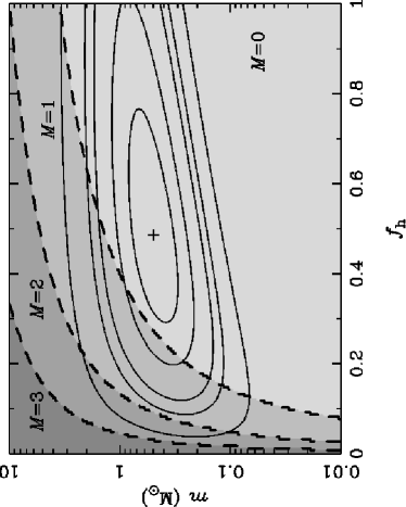
Figure 6: As for figure 3, but for the instance $N=3$. So, this figure assumes that a further binary caustic crossing event has been discovered. The LMC is modeled by a bare disk. Notice that $M=0$ is still the most likely outcome. Irrespective of whether current data indicates $M=1$ or 2, if the next binary caustic crossing event is inferred to be of non-halo origin, it causes difficulties for this model.

In the case where the LMC does not have a halo of its own, figure 6a shows the regions of the $(f_{\rm h},m)$ plane in which the prior expectation is $M=0$ (lightest shaded region), 1, 2 and 3 (darkest shaded region) non-halo events for $N=3$ binary events. Superimposed are the likelihood contours shown in figure 3a derived from the Alcock et al. (1997b) two-year LMC dataset. In reality, even if future datasets concord with the present distribution, the resulting likelihood contours will be somewhat more concentrated about the maximum likelihood solution than indicated in figure 6a. Assuming for the present purposes that the existing likelihood contours still apply, even for a total sample of $N=3$ binary events, the region in which $M=0$ is expected still occupies the largest share of the likelihood. According to the two-year data, we are ten times more likely to inhabit a galaxy in which $M=0$ is the most probable prior than one in which $M=1$ is expected, roughly 370 times more likely than one in which $M=2$ is expected, and 3000 times more likely than one in which $M=3$ is expected. Unless future microlensing events produce a shift in the maximum likelihood lens mass and halo fraction, the dataset is likely to favor even more strongly models with $M=0$ as the most probable prior, since as the number of events grows more of the likelihood will concentrate around the maximum likelihood solution. Figure 6b shows the evolution of the outcome discriminator with threshold ${\cal R}_{*}$ for $N=3$. Clearly, $M=3$ binary events is strongly disfavored by the data, even for models in which such an outcome has a prior relative probability as low as ${\cal R}(3|3)\simeq 0.05$. Current data also argue against models in which $M=2$ has more than a $30\%$ prior relative probability (${\cal R}>0.3$). Irrespective of whether current data indicates $M=1$ or 2, if the next binary caustic crossing event is inferred to be of non-halo origin, it will be difficult to account for it with a minimal Magellanic model. If it is instead found to lie in the Galactic halo, and one of the two current caustic crossing candidates is also confirmed to be of halo origin, then the data would be perfectly consistent with a minimal Magellanic model.

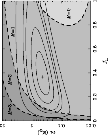
Figure 7: As for figure 6, but using a model for the Magellanic Clouds that includes an enveloping dark halo. The most likely outcome is now $M=1$. Even if a further event is discovered, there is no serious inconsistency whether or not it is found to be caused by a halo or LMC lens.

Figures 7a and 7b show the analogous situation for a maximal Magellanic model (i.e., allowing for the existence of dark Magellanic halos). The difference between figures 6a and 7a is dramatic. Now models in which $M=1$ is the most probable prior contain the overwhelming portion of the likelihood, and models in which $M=0$ is expected occupy only the margins of the likelihood. Integrating the likelihood in each region, we find that we are 55 times more likely to be living in a galaxy in which $M=1$ is expected than one in which $M=0$ is expected, 95 times more likely to be living in such a galaxy than one in which $M=2$ is expected, and 2100 times more likely to be living in such a galaxy than one in which $M=3$ is favored a priori. Again, as the data accumulate it is likely to favor models which predict $M=1$ even more strongly than suggested by figure 7a, assuming the event timescales observed to date are representative of the underlying distribution. The outcome discriminator is shown versus threshold ${\cal R}_{*}$ in figure 7b. As well as confirming the above findings, the figure shows that models in which $M=0$, 1 or 2 have significant prior relative probability ${\cal R}$ are all consistent with the timescales of the current dataset. Even $M=3$ is marginally consistent with our adopted cuts, though it is clearly not strongly favored. If one of the two current binary candidates is of halo origin, then the discovery of another non-halo binary would present no problem for a maximal Magellanic model. Even if the present lenses both reside outside the Galactic dark halo, a third such event would not represent a major crisis for the model, although it would be unexpected. If the third binary event is found to be of halo origin, then there is no problem regardless of the origin of the first two binary events.

9 CONCLUSIONS

The recent discovery of the binary caustic crossing event towards the SMC has provoked intense debate. It seems certain that this event is not caused by a halo lens but rather by one in the SMC itself. This followed the earlier discovery of a binary event towards the LMC, which also may not lie in the halo. Let us stress that there is some uncertainty as to the status of the earlier event. The lens may still come from the halo, rather than the LMC, if the source star is itself binary. There is at most a $10\%$ chance that this is the case. The alternative is that the lens lies in the LMC. Given the measured projected velocity $v_{\rm p}\approx 20\,{\rm km}{\rm s}^{-1}$, then this also has a low prior probability if the velocity dispersion $\sigma$ in the LMC disk is $\mathrel{\hbox to0.0pt{\lower 3.0pt\hbox{$\sim$}\hss}\raise 2.0pt\hbox{$>$}}25\,{\rm km}{\rm s}^{-1}$. This claim is weakened if either the LMC disk is colder or thinner than usually assumed. The ambiguity could be cleared up by multi-epoch spectroscopy of the source. Thus, at least one and maybe both of the events are caused by non-halo lenses. Note that our viewpoint differs from that of Sahu & Sahu (1998), who have claimed that both the binary and the single events seen towards the SMC are caused by self-lensing. As evidence for the single event, they argue that the mass of the lens exceeds 2 ${\rm M}_{\sun}$. Given the absence of any detectable light from the lens in the spectrum of the source, there is no easy explanation of what such an object could be. However, Figure 3 of Afonso et al. (1999) indicates that both the combined MACHO LMC and EROS SMC data are consistent with masses between $0.1$ and 1 ${\rm M}_{\sun}$. In this case, it seems premature to conclude that the lens does not lie in the halo.

In this paper, we have incorporated the valuable information provided by these exotic events into a statistical analysis of the LMC dataset. Given the two binary events, we have calculated the prior probability, as a function of lens mass and halo fraction, that at least one and possibly both are of non-halo origin for standard Galactic and Magellanic Cloud models. The lens mass and halo fraction in these models are themselves constrained by a multi-component likelihood analysis of the microlensing dataset. We develop a new statistic – the “outcome discriminator” – which allows rigorous comparison between the likelihood analysis and the prior expectation. Outcomes in which both binary events lie outside the halo cannot be made consistent with both prior expectation and the LMC dataset. Outcomes in which only one of these events is of non-halo origin provide a reasonable level of consistency. If both events do turn out to be of non-halo origin, then one may be forced to consider alternatives. One possibility is that the Magellanic Clouds themselves are enveloped by their own dark halos. Other alternatives are that the halo may be under-endowed with binaries, or that there is a serious selection bias favoring non-halo lenses (Honma 1999). There is independent support from kinematical studies for the existence of Magellanic halos. Hitherto, the LMC halo has perhaps not received the attention it deserves, especially with regard to modeling. Gould (1993) has shown that an LMC halo could be identified by its microlensing asymmetry, although this does require more than a hundred events. We find that the LMC halo makes a significant contribution to the microlensing optical depth – around a quarter of the total. Honma (1999) has argued that the selection effect is severe, with most halo events missed owing to the typically short time interval between caustic crossings ($<10$ days). This effect assuredly exists, although 10 days is perhaps a little on the long side, allowing for both bad luck and bad weather after the first caustic crossing. A more optimistic figure is perhaps 5 days. However, even if the events are not recognized in real time as binary caustic crossing, they still would be present as unresolved events in the dataset and could be searched for (although of course the projected velocity would not be available).

This paper takes the first steps to include the binary caustic crossing events in the analysis of the microlensing events towards the LMC. Given the modest size and the slow growth of the datasets towards the Magellanic Clouds, it is particularly important to exploit the second-order information provided by such exotic events.

Component	$\sigma/{\rm km}{\rm s}^{-1}$	$\tau/10^{-7}$	$\langle t_{0}\rangle/$days	$\Gamma/10^{-7}\,\mbox{yr}^{-1}$	$N_{\rm exp}(0.35\,{\rm M}_{\sun})$
Galactic halo	$155$	$5.6$	$65\,(m/{\rm M}_{\sun})^{1/2}$	$20.0\,({\rm M}_{\sun}/m)^{1/2}$	$16$
Galactic disk	$30$	$0.06$	$92\,(m/{\rm M}_{\sun})^{1/2}$	$0.14\,({\rm M}_{\sun}/m)^{1/2}$	$0.12$
LMC halo	$55$	$2.1$	$95\,(m/{\rm M}_{\sun})^{1/2}$	$5.1\,({\rm M}_{\sun}/m)^{1/2}$	$4.1$
LMC disk	$25$	$0.54$	$87\,(m/{\rm M}_{\sun})^{1/2}$	$1.4\,({\rm M}_{\sun}/m)^{1/2}$	$1.2$

Table 1: This table gives the velocity dispersion $\sigma$, the optical depth $\tau$, the average timescale (Einstein radius crossing time) $\langle t_{0}\rangle$ and the rate of microlensing $\Gamma$ towards the Large Magellanic Cloud for a number of possible lensing populations. The expected number of events $N_{\rm exp}$ for the 2-year Alcock et al. (1997b) dataset is also given for a lens mass of $0.35\,{\rm M}_{\sun}$, incorporating their efficiencies.

Figure 2: The upper panel shows the distribution of projected velocities $P(v_{\rm p})$ for lenses lying in the Milky Way halo and disk, as well as the LMC halo and disk. Each of the distributions has been normalized so that its maximum lies at unity. As Bennett et al. (1996) already noted, this diagram gives a clean separation between the locations of the lenses. The lower panel assesses the probability of finding a lens with projected velocity as low as $\sim 20\,{\rm km}{\rm s}^{-1}$ as a function of the velocity dispersion of the LMC. The unbroken line refers to a model of the LMC with the standard scale height of $300\,{\rm pc}$ while the broken line is for a super-thin LMC disk with half the standard scale height. The vertical axis is the probability density $P(v_{\rm p}=20)$ measured relative to the most common projected velocity.

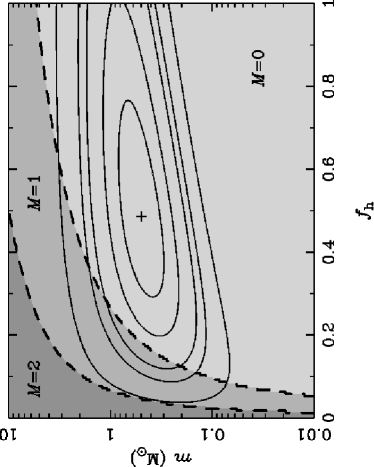
Figure 3: (a) The solid lines show the $34\%$ (innermost), $68\%$, $90\%$, $95\%$ and $99\%$ (outermost) likelihood contours in the plane of lens mass $m$ and halo fraction $f_{\rm h}$ resulting from the Alcock et al. (1997b) 8 event LMC dataset, assuming a combined Galactic (disk+halo) and minimal LMC (disk-only) model. The shaded regions indicate models in which $M=0$, 1 or 2 non-halo binary caustic events are expected from $N=2$ observed caustic crossing binaries. (b) The “outcome discriminator” $D({\cal R}\geq{\cal R}_{*}|t_{i})$ (see main text) as a function of prior relative probability threshold ${\cal R}_{*}$ for the case $N=2$ and $M=0$ (solid line), 1 (dashed line) and 2 (dot-dashed line). The hatched, vertical and horizontal areas respectively denote regions of unacceptably low prior relative probability given the model (${\cal R}<0.1$) and unacceptably low likelihood given the two-year LMC data [$D({\cal R}\geq{\cal R}_{*}|t_{i})<0.1$].

References

- (1) Afonso C.A., et al. 1998, A&A, 337, L17
- (2) Afonso C.A., et al. 1999, A&A, in press
- Albrow et al. (1998) Albrow M.D., et al. 1998, ApJ, 512, 000
- Albrow et al. (1999) Albrow M.D., et al. 1999, ApJ, in press (astro-ph/9807086)
- Alcock et al. (1996) Alcock C., et al. 1996, ApJ, 461, 84
- (6) Alcock C., et al. 1997a, ApJ, 491, 436
- (7) Alcock C., et al. 1997b, ApJ, 486, 697
- Alcock et al. (1999) Alcock C., et al. 1999, ApJ, in press (astro-ph/9807163)
- Bennett (1996) Bennett D.P. et al. 1996 Nucl. Phys. B (Proc. Suppl.), 51B, 131
- Bessell, Freeman & Wood (1986) Bessell M.S., Freeman K.C., Wood P.R. 1986 ApJ, 310, 664
- Duquennoy & Mayor (1991) Duquennoy A., Mayor M. 1991, A&A, 248, 485
- Evans (1995) Evans N.W. 1996, MNRAS, 278, L5
- Evans et al. (1998) Evans N.W., Gyuk G., Turner M.S., Binney J.J. 1998, ApJ, 501, L45
- (14) Griest K. 1991, ApJ, 366, 412
- (15) Griest K., Hu W. 1992, ApJ, 397, 362
- Gould (1992) Gould A. 1992, ApJ, 392, 442
- Gould (1993) Gould A., 1993, ApJ, 404, 451
- Gould (1995) Gould A. 1995, ApJ, 441, 77
- Gould, Bahcall & Flynn (1997) Gould A., Bahcall J.N., Flynn C. 1997, ApJ, 482, 913
- Honma (1999) Honma M. 1999, ApJ, 511, L00
- Jones, Klemola & Lin (1994) Jones B. F., Klemola A.R., Lin D.N.C. 1994, AJ, 107, 1333
- Mao & Paczyński (1991) Mao S., Paczyński B. 1991, ApJ, 347, L37
- Palanque-Delabrouille et al. (1998) Palanque-Delabrouille N., et al. 1998, A&A, 332, 1
- Sahu (1994) Sahu K.C. 1994, Nature, 370, 275
- Sahu & Sahu (1998) Sahu K.C., Sahu M.S. 1998, ApJ, 508, L147
- Schommer et al (1994) Schommer R.A., Olszewski E.W., Suntzeff N.B., Harris H.C. 1992, AJ, 103, 447
- Westerlund (1997) Westerlund B. 1997, The Magellanic Clouds, Cambridge University Press, Cambridge
- Zaritsky & Lin (1997) Zaritsky D., Lin D.N.C. 1997, AJ, 114, 254
- Zhao (1998) Zhao H.S. 1998, MNRAS, 294, 139
- Zombeck (1990) Zombeck M.V. 1990, Handbook of Space Astronomy and Astrophysics, Cambridge University Press (Cambridge), p72