ON THE MASS OF POPULATION III STARS

Abstract

Performing one-dimensional hydrodynamical calculations coupled with nonequilibrium processes for hydrogen molecule formation, we pursue the thermal and dynamical evolution of filamentary primordial gas clouds and attempt to make an estimate on the mass of population III stars. The cloud evolution is computed from the central proton density $n_{c}\sim 10^{2-4}$ cm^-3 up to $\sim 10^{13}$ cm^-3. It is found that, almost independent of initial conditions, a filamentary cloud continues to collapse nearly isothermally due to H₂ cooling until the cloud becomes optically thick against the H₂ lines ($n_{c}\sim 10^{10-11}$ cm^-3). During the collapse the cloud structure separates into two parts, i.e., a denser spindle and a diffuse envelope. The spindle contracts quasi-statically, and thus the line mass of the spindle keeps a characteristic value determined solely by the temperature ($\sim 800$ K), which is $\sim 1\times 10^{3}M_{\odot}$ pc^-1 during the contraction from $n_{c}\sim 10^{5}$ cm^-3 to $10^{13}$ cm^-3. Applying a linear theory, we find that the spindle is unstable against fragmentation during the collapse. The wavelength of the fastest growing perturbation ($\lambda_{\rm m}$) lessens as the collapse proceeds. Consequently, successive fragmentation could occur. When the central density exceeds $n_{c}\,\sim\,10^{10-11}$ cm^-3, the successive fragmentation may cease since the cloud becomes opaque against the H₂ lines and the collapse decelerates appreciably. Resultingly, the minimum value of $\lambda_{\rm m}$ is estimated to be $\sim 2\times 10^{-3}$ pc. The mass of the first star is then expected to be typically $\sim 3M_{\odot}$, which may grow up to $\sim 16M_{\odot}$ by accreting the diffuse envelope. Thus, the first-generation stars are anticipated to be massive but not supermassive.

1 Introduction

Based on the standard Big Bang nucleosynthesis, the first generation of stars should form from materials deficient in heavy elements. In the present-day galaxies, heavy elements or dust grains provide the most efficient cooling mechanism, while the cooling process in primordial gas is likely to be governed by hydrogen molecules. Many authors hitherto have considered the formation processes of primordial stars from metal deficient gas (e.g., Matsuda, Sato, & Takeda 1969; Yoneyama 1972; Hutchins 1976; Silk 1977a, 1977b; Yoshii & Sabano 1979; Carlberg 1981; Struck-Marcell 1982a, 1982b; Lepp & Shull 1983, 1984; Silk 1983; Palla, Salpeter, & Stahler 1983; Yoshii & Saio 1986; Shapiro & Kang 1987; de Araújo & Opher 1989; Uehara et al. 1996; Haiman, Thoul, & Loeb 1996; Omukai et al. 1998). Such first-generation stars, say Population III, could play an important role in the early evolution of galaxies (e.g., Tegmark, Silk, & Blanchard 1994; Ostriker & Gnedin 1996) or the formation of massive black holes (Umemura et al. 1993). Also, they may be responsible for the chemical pollution of intergalactic medium which is recently inferred from metallic absorption in Ly$\alpha$ forest seen in quasar light (Cowie et al. 1995; Songaila & Cowie 1996). It is thus important to study the thermal and dynamical evolution of the primordial gas clouds from which the first-generation stars would form.

If the hydrogen gas were to remain purely atomic, the primordial gas would be cooled down to 10⁴ K due to the Lyman $\alpha$ lines. It is, however, difficult for the gas temperature to become lower, because hydrogen atoms are poor radiator in the lower temperature gas. Therefore, the Jeans mass of such a cloud, which is often referred to the characteristic mass in the star formation theory, becomes much greater than a typical stellar mass. In practice, hydrogen molecules provide key cooling mechanisms. In contrast to the molecule formation on dust grains in metal-rich interstellar gas, the formation of primordial hydrogen molecules can proceed through the gas phase reaction (Saslaw & Zipoy 1967; Peebles &Dicke 1968),

$$e\,+\,{\rm H}\,\rightarrow\,{\rm H}^{-}\,+\,h\nu$$ (1)

$${\rm H}^{-}\,+\,{\rm H}\,\rightarrow\,{\rm H}_{2}\,+\,e$$ (2)

and

$${\rm H}^{+}\,+\,{\rm H}\,\rightarrow\,{\rm H}_{2}^{+}\,+\,h\nu$$ (3)

$${\rm H}_{2}^{+}\,+\,{\rm H}\,\rightarrow\,{\rm H}_{2}\,+\,{\rm H}^{+}.$$ (4)

At high density of $n\,\gtrsim 10^{8}$cm^-3, the molecules can also form through the three-body reactions (Palla et al. 1983),

$$3{\rm H}\,\rightarrow{\rm H}_{2}\,+\,{\rm H}$$ (5)

and

$$2{\rm H}\,+\,{\rm H}_{2}\,\rightarrow\,2{\rm H}_{2}.$$ (6)

Even if a relatively small fraction ($\sim 10^{-3}$) of the molecules form, they make a significant contribution to cooling through the rotational and vibrational transitions, so that the temperature of primordial gas can be reduced to a lower temperature than $10^{4}$K (e.g., Matsuda et al. 1969; Yoneyama 1972; Hutchins 1976; Palla, et al. 1983). Resultantly, the Jeans mass could decrease to stellar mass. However, although a lot of elaborate analyses have been made so far, the masses of Population III stars have not been well converged. Carlberg (1981) and Palla et al. (1983) have shown the Jeans mass can go down to a level of $\lesssim 0.1M_{\odot}$. Yoshii & Saio (1986) derive the initial mass function (IMF) based upon the opacity-limited fragmentation theory (Silk 1977a, 1977b) and find the peak of the IMF around $4-10M_{\odot}$. Uehara et al. (1996) have shown that the minimum masses of the first-generation stars are basically determined by the Chandrasekhar mass, say $\sim 1M_{\odot}$ (see also Rees 1976). In this paper, we reanalyze the formation of Population III stars by computing the collapse of filamentary clouds coupled with H₂ formation.

In the bottom-up scenarios like a cold dark matter (CDM) model, it is expected that the overdense regions with the masses of $10^{5}-10^{7}M_{\odot}$ would first collapse at the redshift range of $10\lesssim z\lesssim 100$ and the first generation of stars would form there. The importance of the H₂ cooling in the collapse of such primordial clouds has been stressed by several authors (e.g., de Araújo & Opher 1989; Haiman et al. 1996; Susa et al. 1996; Tegmark et al. 1997). It has been found in these studies that the mass fraction of H₂ can reach $10^{-4}$ up to $10^{-3}$ and the temperature of the cloud can be reduced to $10^{2}-10^{3}$ K. However, most of the studies are restricted to highly simplified models such as homogeneous pressure-less and/or spherical collapses. In practice, the cloud contraction proceeds inhomogeneously. Since the cloud is more or less nonspherical, the deviation from spherical symmetry grows in time due to its self-gravity until a shocked pancake forms (e.g., Umemura 1993). Recently, several authors have studied the collapse of pregalactic clouds with multi-dimensional hydrodynamical simulations (e.g., Anninos & Norman 1996; Ostriker & Gnedin 1996). Unfortunately they still do not have enough spatial resolution as well as mass resolution to explore the star formation.

The pancake could be gravitationally unstable against fragmentation (e.g., Umemura 1993; Anninos & Norman 1996). It tends to fragment into thin filamentary clouds rather than spherical ones (Miyama, Narita, & Hayashi 1987a, 1987b; Uehara et al. 1996). The filamentary cloud can also fragment into smaller and denser cores (e.g., Larson 1985), in which consequently stars can form. In this paper we thus investigate the thermal and dynamical evolution of the filamentary primordial gas clouds. With using one-dimensional axisymmetric hydrodynamical scheme, we pursue the evolution in the range of more than eighth order of magnitude in density contrast to properly estimate the mass scale of the first-generation stars.

In §2, we describe our model clouds and the computational methods. Numerical results are presented in §3. In §4 we consider the fragmentation of a collapsing filamentary cloud and estimate the mass scale of the fragments and thereby the mass of the first-generation stars. §5 is devoted to the conclusions.

2 MODEL

2.1 Basic Equations

To pursue the thermal and dynamical evolution of a filamentary primordial cloud, we employ a one-dimensional hydrodynamical scheme. We assume that the system is axisymmetric and that the medium consists of ideal gas. The adiabatic index, $\gamma$, is taken to be 5/3 for monatomic gas and 7/5 for diatomic gas. We deal with the following nine species: e, H, H⁺, H^-, H₂, H${}_{2}^{+}$, He, He⁺, and He⁺⁺, The abundance of helium atoms is taken to be 10 % of that of hydrogen by number.

The basic equations are then given in the cylindrical coordinates $(r,\varphi,z)$ by

$${\partial\rho\over\partial t}\,+\,{1\over r}{\partial\over\partial r}(\rho v_{r})\,=\,0\;,$$ (7)

$${\partial\over\partial t}(\rho v_{r})\,+\,{1\over r}{\partial\over\partial r}(r\rho v_{r}^{2})\,+\,{\partial P\over\partial r}\,+\,\rho{\partial\psi\over\partial r}\,=\,0\;,$$ (8)

$${\partial E\over\partial t}\,+\,{1\over r}{\partial\over\partial r}[rv_{r}(E\,+\,P)]\,+\,\rho{\partial\psi\over\partial r}v_{r}\,+\,\Lambda_{\rm net}\,=\,0\;,$$ (9)

$$\triangle\psi\,=\,4\pi G\rho\;,$$ (10)

where

$$\rho\,=\,\sum_{i}\rho_{i}\;,$$ (11)

$$P\,=\,\sum_{i}P_{i}\,=\,\sum_{i}n_{i}kT\;,$$ (12)

$$E\,=\,\sum_{i}\left({P_{i}\over\gamma_{i}\,-\,1}\,+\,{1\over 2}\rho_{i}v_{r}^{2}\right)\;,$$ (13)

where $\rho$, $n$, $v_{r}$, $P$, $\psi$, $E$, $G$, and $k$ are the mass density, number density, radial velocity, gas pressure, gravitational potential, energy per unit volume, gravitational constant, and Boltzmann constant, respectively. The symbol $\Lambda_{\rm net}$ denotes the cooling function which represents the net energy loss rate per unit volume. The values with subscript $i$ denote those of the $i$-th species.

The number density of the $i$-th species, $n_{i}$, is obtained by solving the following time-dependent rate equations,

$${dx_{i}\over dt}\,=\,n_{H}\sum^{9}_{j=1}\sum^{9}_{k=1}k_{jk}x_{j}x_{k}\,+\,n_{H}^{2}\sum^{9}_{l=1}\sum^{9}_{m=1}\sum^{9}_{n=1}k_{lmn}x_{l}x_{m}x_{n}\;,$$ (14)

where $n_{\rm H}$ denotes the total number density of hydrogen nuclei and $x_{i}\,\equiv n_{i}/n_{\rm H}$ is the relative number density of the $i$-th species. The reaction rate coefficients, $k_{jk}$ and $k_{lmn}$, are given in Table 1.

Table 1: REACTION RATE COEFFICIENTS

	Reactions	Rate Coefficients	Reference
(1)	${\rm H}+e\rightarrow{\rm H^{+}}+2e$	$k_{1}=5.85\times 10^{-11}T^{0.5}\exp(-157809.1/T)(1+T_{5}{}^{0.7})^{-1}$	1
(2)	${\rm He}+e\rightarrow{\rm He^{+}}+2e$	$k_{2}=2.38\times 10^{-11}T^{-0.5}\exp(-285335.4/T)(1+T_{5}{}^{0.5})^{-1}$	1
(3)	${\rm He^{+}}+e\rightarrow{\rm He^{++}}+2e$	$k_{3}=5.68\times 10^{-12}T^{0.5}\exp(-631515.0/T)(1+T_{5}{}^{0.5})^{-1}$	1
(4)	${\rm H^{+}}+e\rightarrow{\rm H}+h\nu$	$k_{4}=8.40\times 10^{-11}T^{-1/2}T_{3}{}^{-0.2}(1+T_{6}{}^{0.7})^{-1}$	1
(5)	${\rm He^{+}}+e\rightarrow{\rm He}+h\nu$	$k_{5}=1.9\times 10^{-3}T^{-1.5}\exp(-470000/T)(1+\exp(-94000/T)$	1
		$\hskip 14.22636pt+1.50\times 10^{-10}T^{-0.6353}$
(6)	${\rm He^{++}}+e\rightarrow{\rm He^{+}}\,+\,h\nu$	$k_{6}=3.36\times 10^{-10}T^{-0.5}T_{3}{}^{-0.2}(1+T_{6}{}^{0.7})^{-1}$	1
(7)	${\rm H}+{\rm H}\rightarrow{\rm H}+{\rm H^{+}}+e$	$k_{7}=1.7\times 10^{-4}k_{1}$	2
(8)	${\rm H}+e\rightarrow{\rm H^{-}}+h\nu$	$k_{8}=\left\{\begin{array}[]{ll}1.0\times 10^{-18}T&T\leq 1.5\times 10^{4}{\rm K}\\ {\rm dex}\left[-14.10+0.1175\log T\right.&\\ \hskip 14.22636pt\left.-9.813\times 10^{-3}\right](\log T)^{2}]&T\,>\,1.5\times 10^{4}{\rm K}\end{array}\right.$	3
(9)	${\rm H}+{\rm H^{-}}\rightarrow{\rm H_{2}}+e$	$k_{9}=\left\{\begin{array}[]{ll}1.3\times 10^{-9}&T\leq 10^{4}{\rm K}\\ {\rm dex}\left[-8.78+0.113\log T\right.&\\ \hskip 14.22636pt\left.-3.475\times 10^{-2}(\log T)^{2}\right]&T>10^{4}{\rm K}\end{array}\right.$	3
(10)	${\rm H}+{\rm H^{+}}\rightarrow{\rm H_{2}^{+}}\,+h\nu$	$k_{10}=\left\{\begin{array}[]{ll}1.85\times 10^{-23}T^{1.8}&T\leq 6.7\times 10^{3}{\rm K}\\ 5.81\times 10^{-16}&\\ \hskip 5.69046pt\times(T/56200)^{[-0.6657\log(T/56200)]}&T>6.7\times 10^{3}{\rm K}\end{array}\right.$	3
(11)	${\rm H_{2}^{+}}+{\rm H}\rightarrow{\rm H_{2}}+{\rm H^{+}}$	$k_{11}=6.4\times 10^{-10}$	4
(12)	${\rm H_{2}}+{\rm H}\rightarrow 3{\rm H}$	$k_{12}\;\mbox{[see equation (5) in reference]}$	5
(13)	${\rm H_{2}}+{\rm H^{+}}\rightarrow{\rm H_{2}^{+}}\,+\,{\rm H}$	$k_{13}\,=\,2.4\times 10^{-9}\exp(-21200/T)$	3
(14)	${\rm H_{2}}+e\rightarrow{\rm H}+{\rm H^{-}}$	$k_{14}=2.7\times 10^{-8}T^{-1.5}\exp(-43000/T)$	6
(15)	${\rm H_{2}}+e\rightarrow 2{\rm H}+e$	$k_{15}=4.38\times 10^{-10}T^{0.35}\exp(-102000/T)$	3
(16)	${\rm H_{2}}\,+\,{\rm H_{2}}\,\rightarrow\,2{\rm H}\,+\,{\rm H_{2}}$	$k_{16}\;\mbox{[see equation (5) in reference]}$	5
(17)	${\rm H^{-}}\,+\,e\,\rightarrow\,{\rm H}\,+\,2e$	$k_{17}\,=\,4.0\times 10^{-12}\exp(-43000/T)$	3
(18)	${\rm H^{-}}\,+\,{\rm H}\,\rightarrow\,2{\rm H}\,+\,e$	$k_{18}\,=\,5.3\times 10^{-20}T^{2.17}\exp(-8750/T)$	3
(19)	${\rm H^{-}}\,+\,{\rm H^{+}}\,\rightarrow\,2{\rm H}$	$k_{19}\,=\,7.0\times 10^{-7}T^{-0.5}$	7
(20)	${\rm H^{-}}\,+\,{\rm H^{+}}\,\rightarrow\,{\rm H_{2}^{+}}\,+\,e$	$k_{20}\,=\,\left\{\begin{array}[]{ll}10^{-8}T^{-0.4}&T\,\leq\,10^{4}{\rm K}\\ 4\times 10^{-4}T^{-1.4}\exp(-15100/T)&T\,>\,10^{4}{\rm K}\end{array}\right.$	3
(21)	${\rm H_{2}^{+}}\,+\,e\,\rightarrow\,2{\rm H}$	$k_{21}\,=\,1.68\times 10^{-8}(T/300)^{-0.29}$	8
(22)	${\rm H_{2}^{+}}\,+\,{\rm H^{-}}\,\rightarrow\,{\rm H}\,+\,{\rm H_{2}}$	$k_{22}\,=\,5.0\times 10^{-6}T^{-0.5}$	7
(23)	$3{\rm H}\,\rightarrow\,{\rm H_{2}}\,+\,{\rm H}$	$k_{23}\,=\,5.5\times 10^{-29}T^{-1}$	9
(24)	$2{\rm H}\,+\,{\rm H_{2}}\,\rightarrow\,2{\rm H_{2}}$	$k_{24}\,=\,k_{23}/8$	9

Note. — (1) Cen 1992; (2) Palla et al. 1983; (3) Shapiro & Kang 1987; (4) Karpas, Anicich, & Huntress 1979; (5) Lepp & Shull 1983; (6) Hirasawa 1969; (7) Dalgarno & Lepp 1987; (8) Nakashima, Takayi & Nakamura 1987; (9) Palla et al. 1983

In the models calculated in this paper, the gas temperature does not become far above 10⁴ K. Thus the cooling is dominated by contributions from H at $T\sim 10^{4}$ K and H₂ at $T<10^{4}$ K. We therefore adopt the cooling rate in the form of $\Lambda_{\rm net}=\Lambda_{\rm H}+\Lambda_{\rm H_{2}}+\Lambda_{\rm chem}$, where $\Lambda_{\rm H}$, $\Lambda_{\rm H_{2}}$, and $\Lambda_{\rm chem}$ denote contributions from H, H₂, and chemical reactions, respectively. $\Lambda_{\rm H}$ includes the cooling of H atoms due to recombination, collisional ionization, and collisional excitation (Cen 1992; see also Black 1981). $\Lambda_{\rm H_{2}}$ includes the cooling of H₂ due to rotational and/or vibrational excitations (Lepp & Shull 1983; Haiman et al. 1996), collisional dissociation (Lepp & Shull 1983), and heating due to H₂ formation (Shapiro & Kang 1987). $\Lambda_{\rm chem}$ includes the cooling due to chemical reactions in Table 1 (Shapiro & Kang 1987). For each contribution, we use the analytic formula expressed in each reference. [It is claimed that the cooling rate by Lepp & Shull (1983) is overestimated in relatively low densities ($n_{H}<1{\rm cm}^{-3}$), compared to the rate by Hollenbach & McKee (1989). But, they are in a good agreement with each other in higher densities relevant to the present issue (Galli & Palla 1998).]

When the H₂ density exceeds $\sim 10^{10}$ cm^-3, the H₂ line emission becomes optically thick (Palla et al. 1983). To take account of this effect, we modify the H₂ line cooling with using the photon escape probability (Castor 1970; Goldreich & Kwan 1974): $\Lambda_{\rm H_{2}line}=\beta\Lambda_{\rm H_{2}line,thin}$ and $\beta=(1-e^{-\tau_{R}})/\tau_{R}$, where $\Lambda_{\rm H_{2}line,thin}$ is the cooling function in optically thin regime, $\beta$ is the photon escape probability, and $\tau_{R}$ is the Rossland mean opacity for the H₂ line emission. To evaluate $\tau_{R}$, we determined the level populations with the method of Palla et al. (1983). This type of $\beta$ is applicable rigorously when the gas flows supersonically and its velocity monotonically changes in proportion to the radius (Castor 1970; Goldreich & Kwan 1974). However, the evolution has turned out to depend weakly on the form of $\beta$. Using other types of $\beta$, e.g., $\beta\,=\,e^{-\tau_{R}}$, we have recalculated the evolution and reached basically the same results.

2.2 A Model for a Filamentary Primordial Cloud

In a gravitational instability scenario for the formation of the first structures, a cosmological density perturbation larger than the Jeans scale at the recombination epoch forms a flat pancake-like disk. This process has been extensively studied by many authors (e.g., Zel’dovich 1970; Sunyaev & Zel’dovich 1972; Cen & Ostriker 1992a, 1992b; Umemura 1993). Although the pancake formation is originally studied by Zel’dovich (1970) in the context of the adiabatic fluctuations in baryon or hot dark matter-dominated universes, recent numerical simulations have shown that such pancake structures also emerge in the CDM cosmology (e.g., Cen et al. 1994). Thus, the pancakes are thought to be a ubiquitous feature in gravitational instability scenarios.

In the bottom-up theory like a CDM model, the first collapsed objects at $z\sim 10-100$ are expected to have the masses of $\sim 10^{5-7}M_{\odot}$. In these clouds the gas is heated above $T>10^{3-4}$ K by shock. Therefore, just after the shock formation, the cooling timescale is likely to be shorter than the free-fall one; the temperature of the pancake reduces to the value at which the cooling timescale is comparable to the free-fall one (e.g., Haiman et al. 1996; see also Yoneyama 1972). The temperature of the pancake is then estimated to be $T\simeq 200-1000$ K for $y_{\rm H_{2}}=10^{-4}\sim 10^{-3}$. Thereafter, the pancake is likely to fragment into filamentary clouds which have nearly the same temperature as that of the parent pancake (Miyama et al. 1987a, 1987b; Uehara et al. 1996). In the following we describe a model of a filamentary cloud formed by fragmentation of the pancake.

As a model of a filamentary gas cloud, we assume an infinitely long cylindrical gas cloud for simplicity. At the initial state, we assume the gas to be quiescent and isothermal. We also assume that H^-, H${}_{2}^{+}$, He⁺, and He⁺⁺ do not exist at the start and the relative abundances of other species are spatially uniform for simplicity. The density distribution in the radial direction is set to be

$$\rho\,=\,\rho_{0}\left(1\,+\,{r^{2}\over fR_{\rm fil}^{2}}\right)^{-2}\;,$$ (15)

and

$$R_{\rm fil}\,=\,\sqrt{2kT_{0}\over\pi G\rho_{0}\mu}\;,$$ (16)

where $\rho_{0}$ and $T_{0}$ are respectively the central density and the initial gas temperature, and $f$ represents the degree of deviation from the equilibrium state. A model is specified by the following five parameters: $\rho_{0}$, $T_{0}$, $f$, the electron number fraction $x_{e}$, and the H₂ number fraction $x_{\rm H_{2}}$. When $f\,=\,1$, the cloud is just in hydrostatic equilibrium; the density distribution accords with that of an isothermal filamentary gas cloud in equilibrium (Stodółkiewicz 1963). In this paper, we restrict the parameter $f$ to $f\,\geq\,1$ since we are interested in the evolution of the collapsing clouds.

For the above model, the mass per unit length (line mass) is given by

$$l_{0} = \int^{\infty}_{0}2\pi\rho rdr\,=\,\pi R_{\rm fil}^{2}\rho_{c}f$$ (17)

$$= {2kT_{0}\over\mu G}f=2.2\times 10^{3}\left({f\over 2}\right)M_{\odot}{\rm pc^{-1}}\left({T_{0}\over 1000{\rm K}}\right)\;.$$

Note that the line mass of the equilibrium filamentary cloud depends only on the temperature. When the filamentary cloud forms through gravitational fragmentation of the pancake, its line mass is estimated to be $l\sim 2\rho_{d}\lambda_{m}H_{d}\sim 4kT/(\mu G)$, which is twice that of the equilibrium cloud; i.e., the typical value of $f$ is evaluated to be $f=2$ (Miyama et al. 1987a). Here $\rho_{d}$, $\lambda_{m}$, and $H_{d}$ are the mass density of the parent pancake, the wavelength of the most unstable linear perturbation, and the half thickness of the pancake, respectively. We thus adopt $f=2$ for a typical model.

2.3 Model Parameters and Numerical Method

As shown in §2.2, the initial state is specified by the parameters $n_{0}(\equiv\rho_{0}/\mu$), $T_{0}$, $f$, $x_{e}$, and $x_{\rm H_{2}}$. We examine 60 models, by choosing the parameters $n_{0}$, $T_{0}$, and $f$ to be $n_{0}\,=\,10^{2}$, $10^{3}$, $\cdots$, $10^{6}$ cm^-3, $T_{0}\,=\,10^{2}$, $5\times 10^{2}$, $10^{3}$, $10^{4}$ K, and $f\,=\,2$, 4, 10, respectively. For the parameters $x_{e}$ and $x_{\rm H_{2}}$, we adopt $x_{e}=5\times 10^{-5}$ and $x_{\rm H_{2}}=10^{-4}$ for the models with $T_{0}\,<\,10^{4}$ K. The value of $x_{e}=5\times 10^{-5}$ is adopted from the calculation of Peebles (1968) for the residual post-recombination ionization. [We have found that the results do not depend upon $x_{e}$ as far as $x_{e}\gtrsim 10^{-7}$, because the free electrons could quickly recombine to a level of $x_{e}<10^{-7}$ in the course of the collapse. (see also Haiman, Rees, & Loeb 1996, 1997).] The other abundances are determined by the conservation of mass and charge. For the models with $T_{0}=10^{4}{\rm K}$, we determine the abundances from the statistical equilibrium with e, H, H⁺, He, He⁺, and He⁺⁺.

The hydrodynamic equations (7) - (13) are solved numerically by using the second-order upwind scheme based on Nobuta & Hanawa’s (1998) method. This scheme is an extension of Roe’s (1981) method to the gas having non-constant $\gamma$. [See Nobuta & Hanawa (1998) for more details and the test of the code.] The rate equations (14) are solved numerically with the LSODAR (Livemore Solver for Ordinary Differential equations with Automatic method switching for stiff and non-stiff problems) coded by L. Petzold and A. Hindmarsh.

As for the boundary condition, we take the fixed boundary at $r\,=\,R_{\rm max}$, where $R_{\rm max}$ is the maximum radial coordinate in the computational domain. In all the models we have taken $R_{\rm max}$ to be about ten times greater than the effective radius of the filamentary cloud, $f^{1/2}R_{\rm fil}$. The effect of the fixed boundary is very small. This is because the density is much lower near the outer boundary than at the center, i.e., $\rho\,\lesssim\,10^{-4}\rho_{c}$ for all runs. (In fact, we have calculated the case with larger $R_{\rm max}$ and have confirmed that the numerical results are not changed.)

The numerical grids are non-uniformly distributed so as to enhance the spatial resolution near the center. The grid spacing increases by 5 % for each grid zone with increasing distance from the center. As shown in §3, the characteristic scale shortens in the central high density region as the collapse proceeds. The spatial resolution thus becomes poor near the center. To compute the further contraction with the sufficient spatial resolution, we pursue the subsequent evolution with refining grids. Whenever the number of grid points becomes less than $\sim 20$ within the radius of the half-maximum density ($\rho=0.5\rho_{c}$), we increase the number of grid points and then reposition them on the refined grids in the whole computation region ($0\leq r\leq R_{\rm max}$). The physical variables at the new grid points are determined by linear interpolation. This technique allows us to pursue the dynamical evolution over more than the tenth order of magnitude in the central density.

3 Numerical Results

3.1 Clouds with Intermediate and High Initial Temperatures ($T_{0}\gtrsim 500$ K)

We have examined the evolution of various models with relatively high initial temperature ($T_{0}\gtrsim 500$ K). As a result, the way of the evolution has turned out to be almost insensitive to the model parameters.

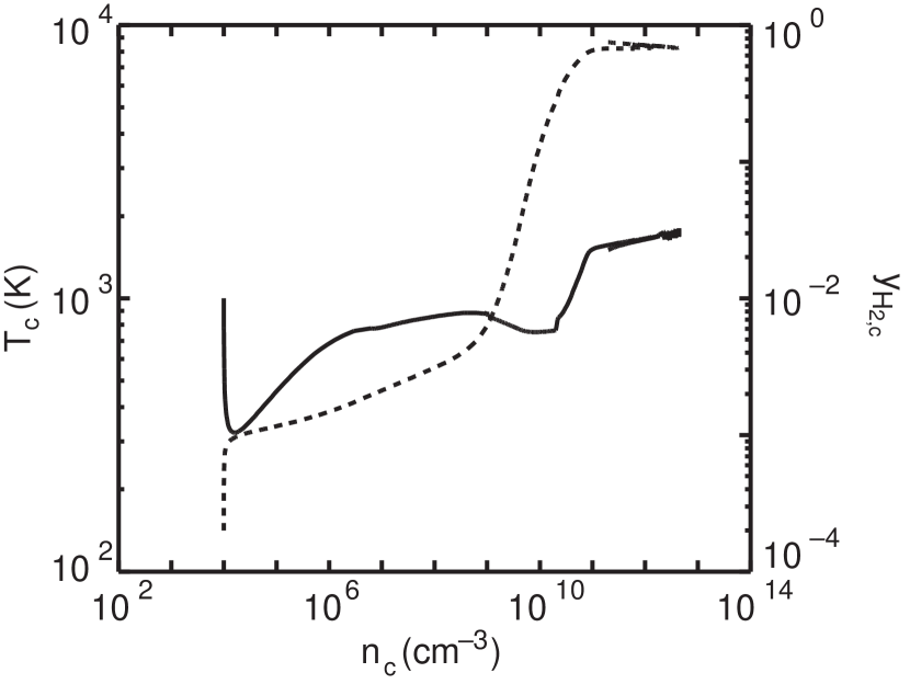
Figure 1: Evolution of the temperature ($T_{c}$, solid curves) and the H₂ abundance ($y_{\rm H_{2},c}$, dashed curves) at the center for the model with $(n_{0},T_{0},f)=(10^{4}\,{\rm cm}^{-3},\ 10^{3}\,{\rm K},\ 2)$. The first prompt decrease of the temperature is due to the H₂ cooling. Afterwards, until the central density reaches $\sim$ 10¹¹ cm^-3, the temperature keeps a nearly constant value of $\sim$ 800 K over the fifth order of magnitude in density. The H₂ abundance steeply rises around $n_{c}\sim 10^{9}$ cm^-3 and reaches $y_{\rm H_{2}}\sim 1$ at the stage at which $n_{c}\sim 10^{11}$ cm^-3. At $n_{c}\sim 10^{11}$ cm^-3, the cloud becomes optically thick against the H₂ lines, and consequently the temperature rises to $\sim$ 1500 K. Thereafter the cloud contraction decelerates near the center and the cloud weakly oscillates around its quasi-static equilibrium state.

As a typical example, we first show the evolution of the model with $(n_{0},\,T_{0},\,f)$ = $(10^{4}\,{\rm cm}^{-3},\,10^{3}\,{\rm K},\,2)$. Figure 1 shows the evolution of the temperature ($T_{c}$) and the mass fraction of H₂ at the center ($y_{\rm H_{2}}\equiv 2x_{\rm H_{2}}$) as a function of the central density $n_{c}$. During the early evolution, H₂ forms mainly through the H^- process [eqs. (1) and (2)]. Because of the effective cooling by the rotational transitions, the temperature first descends promptly to $T\sim 300$ K. When the central density increases to $n_{c}\,\sim\,10^{6}$ cm^-3, the cloud collapses nearly isothermally, staying the temperature at $T\sim 800$ K until the central density reaches $n_{c}\,\sim\,10^{10-11}$ cm^-3. The temperature evolution can be then approximated by $T_{c}\,\propto\,n_{c}^{0.15}$ as far as $n_{c}\,<\,10^{8}$ cm^-3. When the density exceeds $\sim 10^{8}$ cm^-3, the hydrogen molecules form acceleratively through the three-body reactions [eqs. (5) and (6)]. After the central density increases to $n_{c}\,\sim\,10^{11}$ cm^-3, the hydrogen gas is almost completely processed into molecules. Then the cloud becomes optically thick against the H₂ lines and the temperature rises up to $\sim$ 1500 K. At this stage, the cooling time is $50-100$ times longer than the free-fall time. Thereafter the collapse decelerates near the center and the cloud weakly oscillates around its quasi-static equilibrium state.

In Figures 2a - 2d, the time variations of the distributions of the density, the temperature, the H₂ mass fraction, and the contraction time are plotted at several dynamical stages. The contraction time is a dimensionless one, which is defined as $t_{\rm cont}(r)=r/\left[v_{r}(r)t_{\rm ff}\right]$, where $t_{\rm ff}$ is the free-fall time at the center, $t_{\rm ff}\equiv(4\pi G\rho_{c})^{-1/2}$. Since the gravitational force is perceptibly greater than the pressure force at the initial state, the cloud collapses nearly in a free-fall time. When the central density reaches $n_{c}\sim 10^{8}$ cm^-3 ($t=1.434\times 10^{6}$yr), the shock arises around $r\sim 3\times 10^{-2}$ pc, which is characterized by a jump in density and temperature. The shock surface separates the cloud into two parts which correspond to mutually different dynamical states, that is, a denser spindle and a diffuse envelope. During the contraction, the temperature in the spindle keeps nearly constant around $800$ K until the cloud becomes optically thick against the H₂ lines. In the isothermal contraction phase, the outer parts in the spindle exhibit a power-law density distribution, $\rho\propto r^{-2}$. It indicates that the spindle contracts in a self-similar manner. Actually, we have found a similarity solution, which is presented in the Appendix, and it has turned out that the newly found similarity solution well reproduces the numerical results. (See the Appendix for the further detail) At the shock front, the temperature rises up to $T\sim 1500$ K. The contraction time in the spindle is much shorter than that in the envelope. Thus the spindle collapses almost independently of the envelope. When the cloud becomes optically thick against the H₂ lines at the center, the pressure force overwhelms the gravity, so that the second shock forms around $r\sim 2\times 10^{-4}$ pc. After this stage the contraction time of the spindle becomes much longer than $t_{\rm ff}$ and the collapse promptly decelerates.

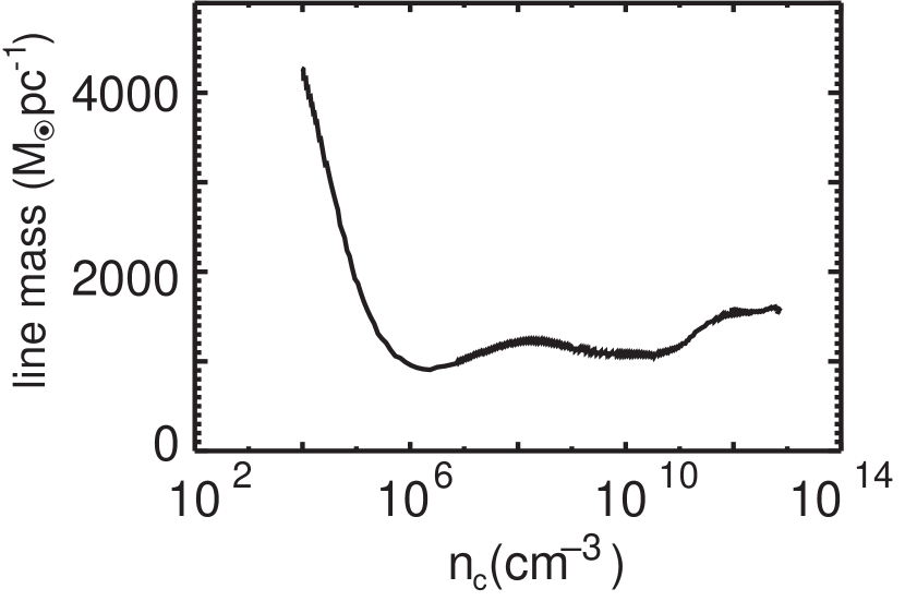
Figure 3: Evolution of the line mass of the spindle in units of $M_{\odot}$ pc^-1 for the model with $(n_{0},T_{0},f)=(10^{4}\,{\rm cm}^{-3},\ 10^{3}\,{\rm K},\ 2)$. The line mass of the spindle keeps a constant value, which is $\sim 10^{3}M_{\odot}$ pc^-1 until the cloud becomes optically thick against the H₂ lines. This value accords with that of an equilibrium isothermal filamentary cloud with the temperature of $T\sim 800$ K. It indicates that in the spindle the gravitational force nearly balances with the pressure force.

Figure 3 shows the evolution of the line mass of the spindle as a function of the central density. We define the line mass as the density integrated over $r$ up to the radius at which the density goes down to one tenth of the central density,

$$l_{\rm sp}\,=\,\int_{0}^{r(\rho=0.1\rho_{c})}2\pi r\rho dr\;.$$ (18)

It is worth noting that during the contraction, the line mass of the spindle keeps a nearly constant value, which is $\sim 1\times 10^{3}M_{\odot}$ pc^-1. This value is close to the line mass of an isothermal filamentary cloud in equilibrium for the temperature of 800 K, i.e., $l_{0}={2kT/\mu G}=0.9\times 10^{3}M_{\odot}{\rm pc^{-1}}\left({T/800{\rm K}}\right)$. It implies that the gravitational force nearly balances with the pressure force in the spindle.

We have found that the evolution is almost independent of the initial parameters, $n_{0}$, $T_{0}$, and $f$, for the models with $T_{0}\gtrsim 500$ K.

3.2 Clouds with Low Initial Temperature ($T_{0}\sim 100$ K)

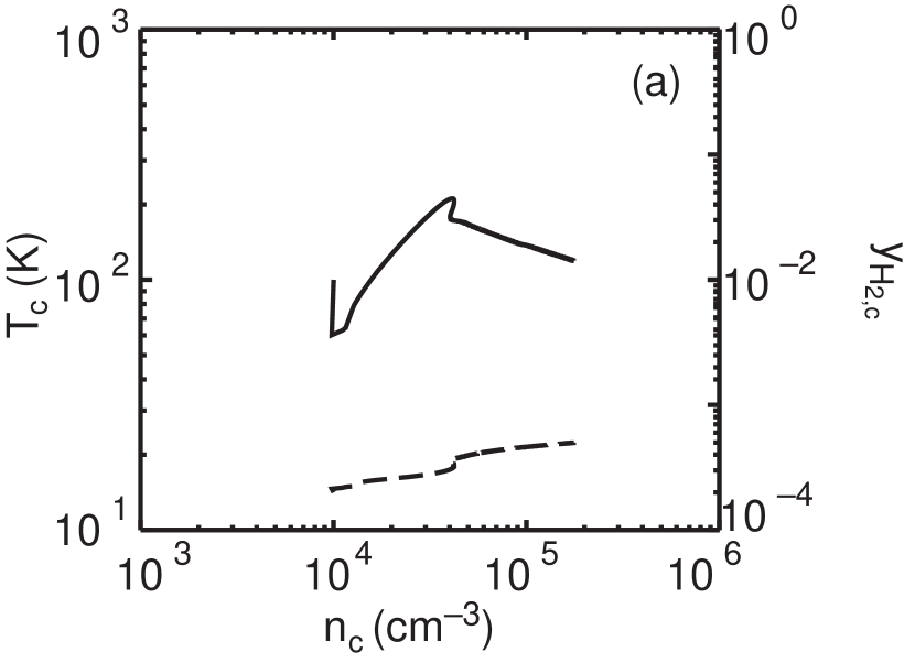
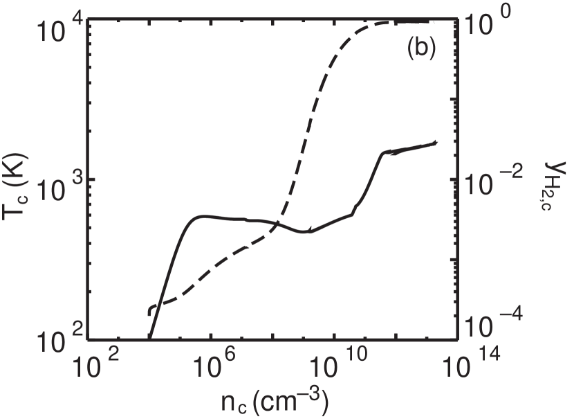
Figure 4: Same as Figure 1 but for the models with (a) $(n_{0},T_{0},f)=(10^{4}\,{\rm cm}^{-3},10^{2}\,{\rm K},\ 2)$ and (b) $(10^{4}\,{\rm cm}^{-3},\ 10^{2}\,{\rm K},\ 10)$. For both models the early evolution is similar; the clouds collapse adiabatically, $T\propto\rho^{2/3}$, because the H₂ line cooling is not effective for such low temperature. For the model with a small $f$ the collapse almost ceases until the central density reaches 10⁵ cm^-3. On the other hand, for the model with a large $f$, the evolution is similar to that of the model with $T_{0}\gtrsim 500$ K. When the cloud temperature exceeds 500 K, the collapse proceeds nearly isothermally due to the H₂ line cooling.

In this subsection, we examine the evolution of models with relatively low initial temperature; $T_{0}\,=\,100$ K. We find that the evolution in the case of low initial temperature depends mainly on the value of $f$. In Figures 4a and 4b, two models with $(n_{0},T_{0},f)$ = $(10^{4}\,{\rm cm}^{-3},\,10^{2}\,{\rm K},\,2)$ and $(10^{4}\,{\rm cm}^{-3},\,10^{2}\,{\rm K},\,10)$ are compared. For both models the early evolution is similar; the clouds collapse adiabatically, $T\propto\rho^{2/3}$, because the H₂ cooling is not effective for $T\lesssim 300$ K. However the later evolution is quite different. For the model with a small $f$, the collapse almost ceases until the central density reaches $10^{5}$ cm^-3. In this case, the contraction time, which is nearly equal to the cooling time, is a hundred times as long as the free-fall time. Hence, the cloud becomes close to the hydrostatic equilibrium with no efficiency of cooling. On the other hand, for the model with a large $f$, the evolution is similar to that of the model with $T_{0}\gtrsim 500$ K. When the cloud temperature exceeds 500 K, the collapse proceeds nearly isothermally due to the H₂ line cooling. In all the models with $T_{0}=100$ K, it has turned out that the evolution proceeds in a similar way dependent upon the value of $f$.

4 Fragmentation of Primordial Gas Clouds

As shown in the previous section, if $T_{0}\gtrsim 500$ K or $f\gtrsim 10$, the filaments collapse quasi-statically, whereas the filaments would not continue to contract if $T_{0}\lesssim 100$ K and $f\lesssim 2$. In the latter case, the filament would be weakly unstable because the length of the realistic filament is shorter than the wavelength of the most unstable mode. Consequently, the filament is likely to contract along the axis without fragmentation. Also, as mentioned in §2.2, the temperature of the initial filaments is estimated to be $T\sim 200-1000$ K in a CDM model. Hence, such low temperature clouds are hardly expected in a CDM scenario. Thus, here we focus on the former case, i.e., a collapsing filament, and consider the hierarchical fragmentation.

The density of a collapsing filament is enhanced by more than eighth order of magnitude, with the constant temperature of $T\sim 800$ K, until the cloud becomes opaque. Thus, the filament could fragment into denser lumps. To diagnose the fragmentation process, we apply a linear theory to the numerical results and thereby estimate the length and mass scales of fragments.

According to the linear theory of an isothermal hydrostatic filament, the perturbation grows most rapidly when its wavelength is about four times longer than the effective cloud diameter. The wavelength and growth rate of the most unstable perturbation depend on the density and temperature of the cloud. Therefore, they change according as the collapse proceeds. In our model of §3.1, the contraction timescale ($t_{\rm cont}$) is longer by a factor of more than five than the free-fall time at the center ($t_{\rm ff}$) after the central density reaches $\sim 10^{6}$ cm^-3. According to Inutsuka & Miyama (1992), when $t_{\rm cont}\gtrsim 10t_{\rm ff}$, the dispersion relation for the collapsing filament is approximated by that of the hydrostatic filament whose scale height is the same as the temporal one of the collapsing cloud, and thus the growth of the density perturbation is approximated by

$$\delta\rho(t)/\rho(t)\,=\,A\exp\left(ik_{z}z\,-\,\int_{0}^{t}i\omega(k_{z},\,t^{\prime})dt^{\prime}\right),$$ (19)

during its linear growth phase, where $k_{z}$ and $\omega$ denote the wavenumber and the frequency of the perturbation, respectively. We thus apply the above equation to our model of §3.1. For the growth rate ($-i\omega$), we use a fitting formula obtained by Nakamura, Hanawa, & Nakano (1993). $A[\,=\,A(k_{z})]$ denotes the initial amplitude of the perturbation. We take $A$ in the form of the power law $A=A_{0}(k_{z}/k_{z,0})^{p}$. When the amplitude of the unstable density perturbation becomes greater than unity ($\delta\rho/\rho\gtrsim 1$), the evolution of the perturbation becomes nonlinear and the cloud will breaks into pieces. It is expected that the evolution of the perturbation depends on the index $p$ and the amplitude $A_{0}$.

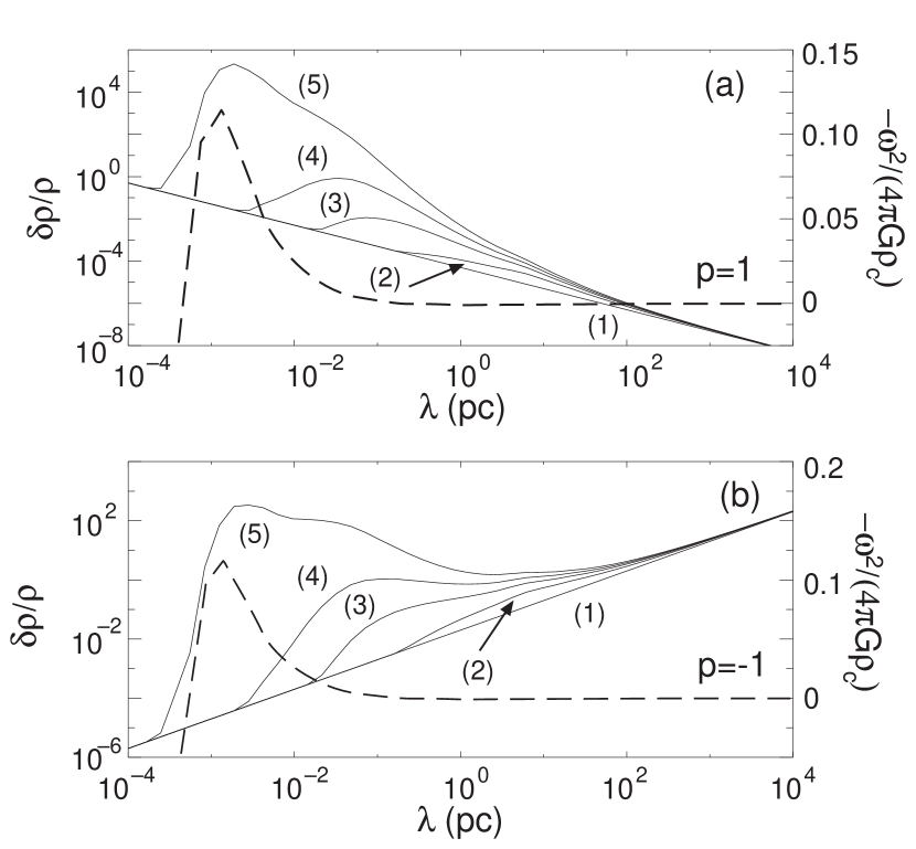
Figure 5: Evolution of density perturbations for the model with $(n_{0},T_{0},f)=(10^{4}\,{\rm cm}^{-3},\ 10^{3}\,{\rm K},\ 2)$. The abscissa and ordinate denote the wavelength and amplitude of the density perturbation, respectively. The initial spectrum of the density perturbations is assumed to be in the form of $A=A_{0}(k_{z}/k_{z,0})^{p}$. The index $p$ is (a) $p=1$ or (b) $p=-1$. We take $(A_{0},k_{z,0})=(1.0\times 10^{-3},1.26\times 10^{2}\,{\rm pc^{-1}})$. The solid curves represent the amplitude of the density perturbations at (1) $t\,=\,0$ yr ($n_{c}\,\simeq\,10^{4}$ cm^-3), (2) $1.384\times 10^{6}$ yr (10⁷ cm^-3), (3) $1.477\times 10^{6}$ yr (10⁹ cm^-3), (4) $1.500\times 10^{6}$ yr (10¹¹ cm^-3), and (5) $1.503\times 10^{6}$ yr ($3\times 10^{12}$ cm^-3), respectively. For comparison, we show the square of the growth rate at the stage (5) with the dashed curves.

Assuming $p=1$ or $p=-1$, we have calculated the time evolution of the density contrast in the filamentary cloud. The results are shown in Figure 5. The solid curves show the density contrast at (1) $t\,=\,0$ yr ($n_{c}\,\simeq\,10^{4}$ cm^-3), (2) $1.384\times 10^{5}$ yr (10⁷ cm^-3), (3) $1.477\times 10^{5}$ yr (10⁹ cm^-3), (4) $1.500\times 10^{5}$ yr (10¹¹ cm^-3), and (5) $1.503\times 10^{5}$ yr ($3\times 10^{12}$ cm^-3), respectively. Here, we have taken $(A_{0},k_{z,0})=(1.0\times 10^{-3},1.26\times 10^{2}{\rm pc^{-1}})$. When $n\lesssim 10^{10-11}$ cm^-3, the wavelength of the fastest growing perturbation is about a hundred times as long as the effective cloud diameter, because of the cumulated growth rate. Hence, the cloud is likely to tear into long filaments before the central density reaches $n_{c}\sim 10^{11}$ cm^-3, if the fluctuations have enough initial amplitudes to enter nonlinear stages. The long filaments shrink further to form thinner filaments. As the shrink proceeds, the wavelength of the fastest growing perturbation shortens. Thus, the filaments may again tear into shorter and denser filaments. Consequently, hierarchical filamentary structures would form, if the initial amplitudes are larger than 0.001 as expected in a CDM cosmology.

When the central density exceeds $n_{c}\sim 10^{11}$ cm^-3, the cloud becomes opaque against the H₂ lines and the collapse quickly decelerates. Hence the hierarchical fragmentation would be terminated. Then the wavelength of the fastest growing perturbation becomes $\lambda_{*}\,\sim\,2\times 10^{-3}{\rm pc}$, which is comparable to that expected from the linear theory of an isothermal filament in equilibrium, as shown by the growth rate in the ending stage in Figure 5. Then, the cloud is most unstable against the perturbation whose wavelength is about four times as large as the effective cloud diameter. This wavelength is nearly independent of the power index $p$ as shown in Figure 5. As a result, the filament is likely to finally fragment into dense cores, the typical mass of which is $\lambda_{*}l_{\rm sp}\sim(2\times 10^{-3}{\rm pc})\times(1.5\times 10^{3}M_{\odot}{\rm pc^{-1}})\sim 3M_{\odot}$. This is the lowest mass of fragments, which provides the minimum core mass for the first-generation stars. The mass possibly increases by accreting the ambient gas. If all the ambient gas within one wavelength of the fastest growing perturbation accretes onto the core, then the core mass increases to $\lambda_{*}l_{0}\sim 16(f/2)(T_{0}/1000\ {\rm K})M_{\odot}$. Thus, the mass of the first stars is expected to be in the range of $3M_{\odot}\lesssim M\lesssim 16(f/2)(T_{0}/1000\ {\rm K})M_{\odot}$. It should be noted that the lower mass as well as the upper mass is not sensitive to the amplitude of the power-law spectrum, because the lower mass is basically determined by the micro process of the H₂ cooling and the upper mass depends only upon the initial temperature.

5 Conclusions

In a wide range of the parameter space, we have numerically explored the thermal and dynamical evolution of filamentary primordial gas clouds with including nonequilibrium process for the H₂ formation. We have found that for the models with $T_{0}\gtrsim 500$ K or $f\gtrsim 10$, the collapse proceeds nearly isothermally due to the H₂ line cooling, staying the temperature at $T\sim 800$ K. During the contraction, the cloud structure is divided into two parts, i.e., a spindle and an envelope. The line mass of the spindle keeps a nearly constant value of $\sim 1\times 10^{3}M_{\odot}$ pc^-1 during the contraction from $10^{6}$ cm^-3 to $10^{11}$ cm^-3. The outer part in the spindle exhibits a power-law density distribution as $\rho\propto r^{-2}$. This behavior is well reproduced by a newly found self similar solution. When the central density reaches $n_{c}\gtrsim 10^{11}$ cm^-3, the cloud becomes opaque against the H₂ line cooling and reaches a quasi-static equilibrium state with keeping the line mass. On the other hand, for the models with $T_{0}\sim 100$ K and $f\lesssim 2$, the cloud contraction is much slower because the H₂ cooling is not effective. The contraction immediately ceases. In a CDM scenario, the former case (collapsing filaments) would be more probable.

Applying a linear theory for the gravitational instability of collapsing filaments, we find that the spindle is unstable against fragmentation during the quasi-static contraction. The wavelength of the fastest growing perturbation ($\lambda_{\rm m}$) lessens as the collapse proceeds. Thus successive fragmentation could occur. When the central density exceeds $n_{c}\,\sim\,10^{11}$ cm^-3, the successive fragmentation may be suppressed since the cloud becomes opaque against the H₂ lines and the collapse promptly decelerates. Resultingly, the minimum value of $\lambda_{\rm m}$ is estimated to be $\sim 2\times 10^{-3}$ pc. The typical mass of the first stars is then expected to be $\sim 3M_{\odot}$, which may grow up to $16M_{\odot}$ by accreting the diffuse envelope. The present results may be relevant to the early evolution of primordial galaxies and the metal enrichment of the intergalactic space.

Appendix A Similarity Solutions of A Polytropic Filamentary Cloud

As mentioned in §3, the spindle seems to collapse self-similarly during the nearly isothermal contraction phase from $n_{c}\sim 10^{6}$ cm^-3 to 10¹¹ cm^-3; e.g., the density distribution of the spindle is characterized by the power-law distribution of $\rho\propto r^{-2}$. But this behavior is different from that of the similarity solution ($\rho\propto r^{-4}$) of an isothermal filamentary cloud that is known so far (Miyama et al. 1987a; see also eqs. [A18] and [A19]). In this appendix we seek another type of similarity solutions in more generic equations of state.

We consider an infinitely long cylindrical cloud in which the density is uniform along the axis. We assume the gas to be polytropic; $P=K\rho^{\gamma}$, where $K$ is constant. The equation of motion and the continuity equation are then described as

$${\partial v_{r}\over\partial t}+v_{r}{\partial v_{r}\over\partial r}+{2Gl\over r}+{1\over\rho}{\partial P\over\partial r}=0\;,$$ (A1)

$${\partial l\over\partial t}+2\pi r\rho v_{r}=0\;,$$ (A2)

and

$${\partial l\over\partial r}-2\pi r\rho=0\;,$$ (A3)

where $l$ denotes the line mass (mass per unit length) contained within a radius $r$.

We now look for a similarity solution of the form

$$x={r\over at}\;,$$ (A4)

$$\rho(r,t)={\tilde{\rho}(x)\over 2\pi Gt^{2}}\;,$$ (A5)

$$v_{r}(r,t)=a\tilde{v}_{r}(x)\;,$$ (A6)

$$l(r,t)={a^{2}\over 2G}\tilde{l}(x)\;,$$ (A7)

and

$$a=t^{1-\gamma}\sqrt{K(2\pi G)^{1-\gamma}}\;,$$ (A8)

where the physical variables with a tilde denote those in the similarity coordinate, $x$. Substituting equations (A4) $-$ (A8) into equations (A1) $-$ (A3), we obtain

$${d\tilde{\rho}\over dx}={Y(x,\tilde{\rho},\tilde{v}_{r})\over X(x,\tilde{\rho},\tilde{v}_{r})}\;,$$ (A9)

$${d\tilde{v}_{r}\over dx}={Z(x,\tilde{\rho},\tilde{v}_{r})\over X(x,\tilde{\rho},\tilde{v}_{r})}\;,$$ (A10)

$$X(x,\tilde{\rho},\tilde{v}_{r})=[\tilde{v}_{r}-(2-\gamma)x]^{2}-\gamma{\tilde{\rho}}^{\gamma-1}\;,$$ (A11)

$$Y(x,\tilde{\rho},\tilde{v}_{r})=-\left[\tilde{v}_{r}-(2-\gamma)x\right]^{2}\left[{\tilde{\rho}^{2}\over\gamma-1}+(2x-\tilde{v}_{r}){\tilde{\rho}\over x}\right]-(\gamma-1)\tilde{\rho}\tilde{v}_{r}\;,$$ (A12)

and

$$Z(x,\tilde{\rho},\tilde{v}_{r})=-[\tilde{v}_{r}-(2-\gamma)x]^{2}{\tilde{\rho}\over\gamma-1}+(\gamma-1)\tilde{v_{r}}[\tilde{v}_{r}-(2-\gamma)x]+{\gamma\tilde{\rho}^{\gamma-1}\over x}(\tilde{v}_{r}-2x)\;.$$ (A13)

Note that equations (A9) through (A13) have a singularity at $\gamma=1$ (A polytropic sphere has a singularity at $\gamma=4/3$. This is fundamentally the same as the dynamical stability condition of the sphere.).

One of the solutions of equations (A9) through (A13) is expressed as

$$\tilde{v}_{r}=0$$ (A14)

and

$$\tilde{\rho}=\left[{(2-\gamma)^{2}\over 2\gamma(1-\gamma)}\right]^{1\over\gamma-2}x^{-{2\over 2-\gamma}}\;.$$ (A15)

In this solution the gas is at rest and the density diverges at the origin. This solution corresponds to a singular equilibrium solution for a polytropic filamentary cloud.

A regular solution at $x=0$ has an asymptotic behavior,

$${d\ln\tilde{\rho}\over d\ln x}=-{2\over 2-\gamma}$$ (A16)

and

$${d\ln\tilde{v}_{r}\over d\ln x}=-{2(\gamma-1)\over 2-\gamma}\;.$$ (A17)

Thus, when the value of $\gamma$ is nearly equal to unity, the density and velocity distributions follow $\rho\rightarrow r^{-2}$ and $v_{r}\rightarrow{\rm const.}$ in the outer region of $|x|\gg 1$. This behavior is quite similar to that of a sphere (Larson 1969; Penston 1969). Note that this similarity solution exists only for $\gamma<1$. This is essentially the same as the dynamical stability condition of the polytropic cylinder. This similarity solution has different characteristics from a singular case of $\gamma=1$. In the similarity solution of $\gamma=1$, the density and velocity distributions are given as (see Miyama et al. 1987a)

$$\tilde{\rho}={4\over(1+x^{2})^{2}}\;,$$ (A18)

and

$$\tilde{v}_{r}=x\;,$$ (A19)

which are proportional to $x^{-4}$ and $x$, respectively, in the region of $|x|\gg 1$.

In Figure 6 the similarity solutions of $\gamma=0.9$ and 0.99 are compared with that of $\gamma=1$. The thick and thin solid curves represent the density and velocity distributions of the similarity solutions with $\gamma\neq 1$, respectively. The dashed curves are the similarity solution of $\gamma=1$ (Miyama et al. 1987a). The newly found similarity solution seems to well reproduce the numerical results during the nearly isothermal contraction phase; the density distribution in the outer part in the spindle is nearly proportional to $r^{-2}$ and the velocity distribution is proportional to $r$ near the center [see Fig. 2. Recently Kawachi & Hanawa (1998) also studied the gravitational collapse of a polytropic cylinder and confirmed that the evolution of the cylinder converges to the similarity solution.]. It should be stressed again that whether $\gamma$ is precisely unity or not transforms conclusively the self-similar manner. The present similarity solution for $\gamma\neq 1$ is likely to be applicable for the realistic situations.

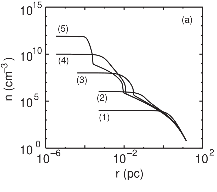
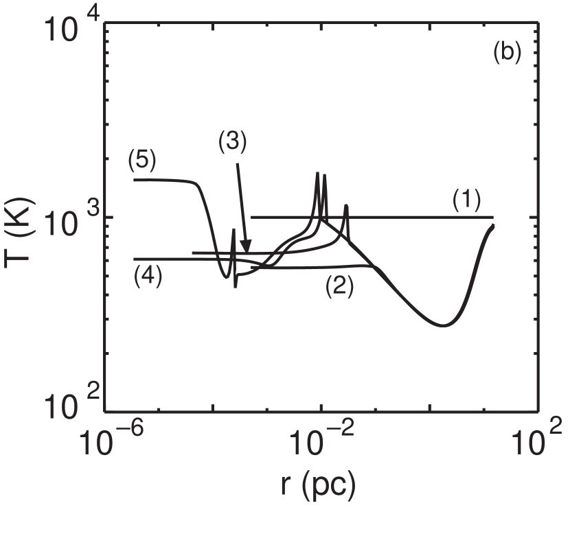
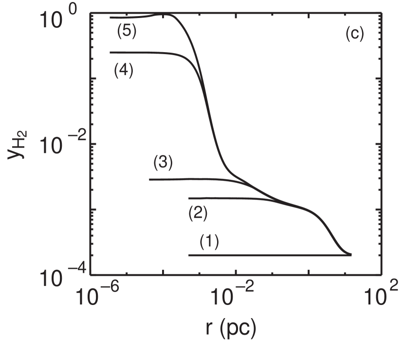
Figure 2: Time variations of the distributions for (a) the density, (b) the temperature, (c) the H₂ abundance, and (d) the contraction time are shown for the same model as Fig. 1, i.e., $(n_{0},T_{0},f)=(10^{4}\,{\rm cm}^{-3},\ 10^{3}{\rm K},\ 2)$. They are plotted at the stages at which (1) $t=0$ yr ($n_{c}=10^{4}$) cm^-3, (2) $t=1.285\times 10^{6}$ yr ($n_{c}=10^{6}$ cm^-3), (3) $t=1.434\times 10^{6}$ yr ($n_{c}=10^{8}$ cm^-3), (4) $t=1.496\times 10^{6}$ yr ($n_{c}=10^{10}$ cm^-3), and (5) $t=1.502\times 10^{6}$ yr ($n_{c}=10^{12}$ cm^-3).

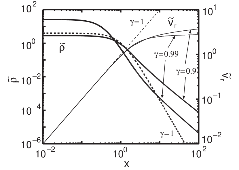
Figure 6: Similarity solutions of filamentary clouds with $\gamma=0.9$ and 0.99. The thick and thin solid curves show the density and velocity distributions in the similarity coordinates, respectively. For comparison, we denote the density and velocity distributions of the isothermal similarity solution with the thick and thin dashed curves, respectively. For the similarity solutions with $\gamma=0.9$ and 0.99, the density distribution is nearly proportional to $r^{-2}$ and the velocity converges to a constant value in the outer part.

References

- (1) Anninos, P. A. & Norman, M. L. 1996, ApJ, 460, 556
- (2) Carlberg, R. G. 1981, MNRAS, 197, 1021
- (3) Castor, J. I. 1970, MNRAS, 149, 111
- (4) Cen, R. 1992, ApJ, 78, 341
- (5) Cen, R., Miralda-Escude, J., Ostriker, J. P., & Rauch, M. 1994, ApJ, 437, L9
- (6) Cen, R., & Ostriker, J. P. 1992a, ApJ, 393, 22
- (7) ———-. 1992b, ApJ, 399, 331
- (8) Cowie, L. L., Songaila, A., Kim, T-S, & Hu, E. M. 1995, AJ, 109, 1522
- (9) Dalgarno, A., & Lepp, S. 1987, in Astrochemistry, ed. M. S. Varya & S. P. Tarafdar (Dordrecht:Reidel), p. 109
- (10) de Araújo, J. C. N. & Opher, R. 1989, MNRAS, 239, 371
- (11) Galli, D. & Palla, F. 1998, A&A, 335, 403 (astro-ph/9803315)
- (12) Goldreich, P. & Kwan, J. 1974, ApJ, 189, 441
- (13) Haiman, Z., Rees, M. J., & Loeb, A. 1996, ApJ, 467, 522
- (14) ———-. 1997, ApJ, 476, 458
- (15) Haiman, Z., Thoul, A. A., & Loeb, A. 1996, ApJ, 464, 523
- (16) Hirasawa, T. 1969, Prog. Theor. Phys., 42, 523
- (17) Hollenbach, D. & McKee, C. F. 1989, ApJ, 342, 306
- (18) Hutchins, J. B., 1976, ApJ, 205, 103
- (19) Inutsuka, S. & Miyama, S. M. 1992, ApJ, 388, 392
- (20) Karpas, Z., Anicich, V., & Huntress, W. T. 1979, J. Chem. Phys., 70, 2877
- (21) Kawachi, T. & Hanawa, T. 1998, submitted to PASJ
- (22) Larson, L. 1969, MNRAS, 145, 271
- (23) —–. 1985, MNRAS, 214, 379
- (24) Lepp, S. & Shull, M. 1983, ApJ, 270, 578
- (25) —–. 1984, ApJ, 280, 465
- (26) Matsuda, T., Sato, H., & Takeda, H. 1969, Prog. Theor. Phys., 42, 219
- (27) Miyama, S. M., Narita, S. & Hayashi, C. 1987a, Prog. Theor. Phys., 78, 1051
- (28) —–. 1987b, Prog. Theor. Phys., 78, 1065
- (29) Nakamura, F., Hanawa, T., & Nakano, T. 1993, PASJ, 45, 551
- (30) Nakashima, K., Takayi, H., & Nakamura, H. 1987, J. Chem. Phys., 86, 726
- (31) Nobuta, K. & Hanawa, T. 1998, submitted to ApJ
- (32) Omukai, K, Nishi, R., Uehara, H., & Susa, H. 1998, Prog. Theor. Phys., 99, 747
- (33) Ostriker, J. P. & Gnedin, N. Y. 1996, ApJ, 472, L63
- (34) Palla, F., Salpeter, E. E., & Stahler, S. W., 1983, ApJ, 271, 632
- (35) Peebles, P. J. E. 1968, ApJ, 153, 1
- (36) Peebles, P. J. E. & Dicke, R. H. 1968, ApJ, 154, 891
- (37) Penston, M. V. 1969, MNRAS, 144, 425
- (38) Rees, M. J. 1976, MNRAS, 176, 483
- (39) Roe, P. L. 1981, J. Comput. Phys. 43, 357
- (40) Saslaw, W. C. & Zipoy, D. 1967, Nature, 216, 976
- (41) Shapiro, P. R. & Kang, H. 1987, ApJ, 318, 32
- (42) Silk, J. 1977a, ApJ, 211, 638
- (43) ——. 1977b, ApJ, 214, 152
- (44) ——. 1983, MNRAS, 205, 705
- (45) Songaila, A. & Cowie, L. L. 1996, AJ, 112, 335
- (46) Stodółkiewicz, J.S. 1963, Acta Astron., 13, 30
- (47) Struck-Marcell, C. 1982a, ApJ, 259, 116
- (48) —–. 1982b, ApJ, 259, 127
- (49) Sunyaev, R. A. & Zel’dvich, Ya. B. 1972, A&A, 20, 189
- (50) Susa, H., Uehara, H., & Nishi, R. 1996, Prog. Theor. Phys., 96, 1073
- (51) Tegmark, M., Silk, J. & Blanchard, A. 1994, ApJ, 420, 484
- (52) Tegmark, M., Silk, J., Rees, M., Blanchard, A., Abel, T., & Palla, F. 1997, ApJ, 474, 1
- (53) Yoneyama, T. 1972, PASJ, 24, 87
- (54) Yoshii, Y. & Sabano, Y. 1979, PASJ, 32, 229
- (55) Yoshii, Y. & Saio 1986, ApJ, 301, 587
- (56) Uehara, H., Susa, H., Nishi, R., & Yamada, M. 1996, ApJ, 473, L95
- (57) Umemura, M., Loeb, A., & Turner, E. 1993, ApJ, 419, 459
- (58) Umemura, M. 1993, ApJ, 406, 361
- (59) Zel’dovich, Ya. B. 1970, A&A, 5, 84