Simulating Large-scale Structure

Abstract

ABSTRACT. After two decades of direct dynamical simulation of large–scale structure in the universe, it is safe to say the subject is now “mature”. Still, there are parts of the problem that are less well developed than others. In general, the collisionless dynamics of the dark matter component is better understood than the collisional gas dynamics of the baryonic component. In situations where the gas dynamics is relatively simple, such as the Lyman–$\alpha$ forest and the intracluster medium in X–ray clusters, our ability to reproduce observational data has evolved rapidly, and the interpretive and predictive power of such experiments should now be taken seriously. A comparison of twelve gas dynamic codes to the problem of forming a single X–ray cluster shows that numerical inaccuracies are modest (typically below ten percent), leaving missing physics as the main source for large systematic differences between theory and observation. Galaxy formation, being more complex, is farther behind in its development, but simulations capable of resolving the morphological range of the Hubble sequence in cosmologically interesting volumes may be just around the corner.

ABSTRACT. After two decades of direct dynamical simulation of large–scale structure in the universe, it is safe to say the subject is now “mature”. Still, there are parts of the problem that are less well developed than others. In general, the collisionless dynamics of the dark matter component is better understood than the collisional gas dynamics of the baryonic component. In situations where the gas dynamics is relatively simple, such as the Lyman–$\alpha$ forest and the intracluster medium in X–ray clusters, our ability to reproduce observational data has evolved rapidly, and the interpretive and predictive power of such experiments should now be taken seriously. A comparison of twelve gas dynamic codes to the problem of forming a single X–ray cluster shows that numerical inaccuracies are modest (typically below ten percent), leaving missing physics as the main source for large systematic differences between theory and observation. Galaxy formation, being more complex, is farther behind in its development, but simulations capable of resolving the morphological range of the Hubble sequence in cosmologically interesting volumes may be just around the corner.

1 Introduction

Building a universe in the laboratory is a daunting, if perversely inviting (think of the funding levels!), proposition. Fortunately for astrophysicists, there are interesting physical questions about the universe that can be addressed without the creation of a bona fide mock-up — a reasonable facsimile will do. How “reasonable” the facsimile needs to be is dependent on the level of detail of the questions being posed and the complexity of the physics driving the processes at hand. In this contribution, I will briefly review the status of attempts at producing virtual facsimiles of our real universe through direct numerical simulation. In particular, I’ll focus on the formation of large–scale structure (LSS), where “large” means galactic scales and upward. Sub–galactic scale evolution, notably the Lyman–$\alpha$ forest, is reviewed by Weinberg et al. in this volume. The reader will note a general theme which is both historical and epistemological; “simpler” parts of the problem which have been worked on for the longest time are better understood than the more difficult aspects which are only now receiving careful attention.

2 N-body Models of LSS

On it’s largest scales, structure in the matter component of the universe is driven by gravity. The first attempts at direct N-body modeling of the gravitational instability process in a volume of cosmic scale (Aarseth, Turner & Gott 1979) revealed morphological features — clusters, walls and voids — characteristic of the observed large–scale galaxy distribution. Future experiments enlarged the simulated volumes and increased the resolving power, leading to the current view of an evolving “cosmic web” of dark matter as seen in the images from the set of $256^{3}$ particle Virgo simulations (Jenkins et al. 1998) shown many times at this meeting. Since 1970, advances in computing technology — faster processors, more memory, better algorithms — have allowed the typical number of particles in cosmological simulations to increase by a factor of 100 every decade. The increased dynamic range has been exploited in two orthogonal directions which can be roughly characterised as increased volume at fixed resolution (minimum mass/length scales) or increased resolving power (smaller minimum mass/length scales) at fixed simulated volume.

Table 1: Hubble Volume Models. Periodic cubes of side $L$ are simulated using CDM fluctuation spectra with shape parameter $\Gamma\!=\!0.21$ and normalizations $\sigma_{8}$ listed. The redshifts correspond to look–back epochs along the box diagonal $z_{\sqrt{3}L}$, box side length $z_{L}$ and half-length $z_{L/2}$ for the light–cone datasets.

Model	$\Omega_{m}$	$\Omega_{\Lambda}$	$\sigma_{8}$	$L$	$z_{\sqrt{3}L}$	$z_{L}$	$z_{L/2}$
$\tau$CDM	1.0	0.0	0.60	2000	4.6	1.3	0.45
LCDM	0.3	0.7	0.90	3000	4.4	1.5	0.58

2.1 The Hubble Volume Project

The natural progression toward simulating ever larger volumes has a practical endpoint — the entire visible universe. Though past experimenters could have arbitrarily enlarged their volumes to encompass the Hubble length $c{\rm H_{o}}^{-1}\!=\!3000\hbox{$\,h^{-1}$}{\rm\ Mpc}$, the lack of ability to resolve structure out of the linear regime of fluctuations left the exercise empty. Why simulate an analytic system? Parallel computers, with their large pools of multi–processor memory capable of supporting very large $N$ calculations, have changed the situation dramatically. Using 32–bit numerics, the phase space position plus an index (useful in post-processing) for $10^{9}$ particles requires 28 Gb of memory. A parallel machine with 512 nodes each with 128 Mb of memory offers 65 Gb, enough for $10^{9}$ particles with space left over for additional large arrays needed for bookkeeping and gravitational potential calculations. What will a billion particles do for you? Suppose we ask that the particle mass be sufficiently small that the Coma cluster (mass $\sim 1.1\times 10^{15}\hbox{$\,h^{-1}$}{\rm M}_{\odot}$) be resolved by 500 particles. Then the mass associated $10^{9}$ particles, $M_{tot}\!=\!2.2\times 10^{21}\hbox{$\,h^{-1}$}{\rm M}_{\odot}$, would fill cubes of length $2000\hbox{$\,h^{-1}$}{\rm\ Mpc}$ for $\Omega_{m}\!=\!1$ and $3000\hbox{$\,h^{-1}$}{\rm\ Mpc}$ for $\Omega_{m}\!=\!0.3$. Since the diagonals of these cubes contain independent information on a length scale exceeding the Hubble length, they have a legitimate claim to be considered simulations of the “Hubble Volume”. Simulations using a billion particles in such Gpc sized volumes have now been performed by the Virgo Consortium using a message–passing version of the Hydra N–body code (MacFarland et al. 1998) run on a 784 processor SGI/Cray T3E at the Rechenzentrum Garching. The runs each took roughly 5 days of cpu time on 512 processors (equivalent to 7 years of single–cpu computing) and each generated $\sim 200Gb$ of output data. With such a large simulated volume, the traditional method of recording images of the mass distribution at fixed intervals of world time is of little value for addressing questions of observational significance. Observational data comes to us from our past light–cone, so generating output along the past light–cone of artificial “observers” in the simulated volume is a natural solution. The Hydra code was modified to propagate output filters through the volume, creating “surveys” with different amounts of “sky coverage” to the depths listed in Table 1. Details of the geometries of the light cone output is available on the web, and a gif image of the “Hubble tie”, a $40\hbox{$\,h^{-1}$}{\rm\ Mpc}$ thick slice along the diagonal wedge survey of the $\tau$CDM model can also be found there. This image, displayed in large format in the foyer of the MPA building during the meeting, reveals clearly the emergence of large–scale structure in the universe from $z\simeq 5$ to the present.

Figure 1: Cumulative number of clusters identified in the Hubble Volume models at the final epoch.

Figure 1 shows the number of clusters found in each of the simulated models at the present epoch. The shear number of collapsed objects — roughly 3000 clusters at least as massive as Coma and nearly one million clusters resolved by more than 32 particles — allows detailed investigation of statistical questions such as the behavior of the cluster–cluster correlation function with cluster richness (Colberg et al. 1998). Very rare events can also be studied. In the $\tau$CDM model at the present epoch, the largest group identified with a standard percolation technique lies in a region where there are four clusters each more massive than Coma lying within a cube of side $20\hbox{$\,h^{-1}$}{\rm\ Mpc}$! No obvious counterpart in our local universe comes to mind (the Great Attractor region may come close), but future deep X–ray, Sunyaev–Zel’dovich and gravitational lensing studies should discover such rarities.

Figure 2: Positions of clusters in the 100 sq deg diagonal wedge light–cone survey from the $\tau$CDM model. Numbers indicate redshift.

A view of clusters resolved by at least 32 particles ($M\geq 7.0\times 10^{13}\hbox{$\,h^{-1}$}{\rm M}_{\odot}$) and located in the $10\times 10$ square degree light–cone survey along the cube diagonal of the $\tau$CDM run is shown in Figure 2. The plot shows positions in the background Robertson–Walker metric (the space of the computation) and the linear extent of the image is 2400 $\,h^{-1}$  Mpc. All the spatial information in the image is formally independent; no periodic replications are used to generate the map.

Figure 3: Characteristics of the 1313 clusters displayed in Figure 2. The minimum mass of $7\times 10^{13}\hbox{$\,h^{-1}$}{\rm M}_{\odot}$ corresponds to 32 particles. See the text for discussion.

A total of 1313 clusters exist in the field, the furthest located at redshift $z\!=\!1.68$. The emergence of clusters at $z\mathrel{\hbox to0.0pt{\lower 3.0pt\hbox{$\mathchar 536\relax$}\hss}\raise 2.0pt\hbox{$\mathchar 316\relax$}}1$ is evident from the enhancement in number density toward the vertex. Hints of the filamentary large–scale matter network are visible at moderate redshift, but at high redshift the thickness of the wedge approaches $200\hbox{$\,h^{-1}$}{\rm\ Mpc}$ and projection effects blend together the coherent features which have characteristic length scale $\sim 40\hbox{$\,h^{-1}$}{\rm\ Mpc}$. Basic observables of this cluster population are displayed in Figure 3. The panels show the line–of–sight velocity of the cluster center of mass, the one–dimensional velocity dispersion $\sigma_{1D}$ and the cluster mass identified using a friends–of–friends percolation algorithm with linking length 0.2 times the mean interparticle separation in the comoving metric. A surprising result from this figure is the fact that the cluster with the third highest velocity dispersion in the sample is also the most distant object at $z\!=\!1.68$. The one-dimensional velocity dispersion of $\sigma_{1D}\!=\!1072\hbox{ km s${}^{-1}$}$ translates into an intracluster medium temperature $kT\!=\!6.3{\rm\ keV}$, assuming a ratio of specific energies $\sigma_{1D}^{2}/(kT/\mu m_{p})\!=\!1.17$, (Frenk et al. 1998). The thermal Sunyaev–Zel’dovich (SZ) effect from such a cluster should be readily observable (see §3 below). The existence of such a potential well at this redshift provides hope that such targets will begin to appear in deep observational searches for clusters using SZ, weak gravitational lensing, and even direct X–ray detection (which must fight $(1+z)^{4}$ surface brightness dimming). A few examples of clusters with $z>1$ have emerged, including a system discovered optically, CIG J0848+4453, lying at $z\!=\!1.273$ with a velocity dispersion $\sigma_{1D}\!=\!700\pm 180\hbox{ km s${}^{-1}$}$ based on 8 galaxy spectra (Stanford et al. 1997). Deep ROSAT HRI images of regions centered on high redshift radio galaxies have also provided distant cluster candidates, among them 3C294 at $z\!=\!1.786$ (Dickinson, private communication). The upper panel in Figure 3 shows the line–of–sight (los) mean peculiar velocity $v_{z}$ of the clusters as a function of redshift. This quantity is observable via the kinematic SZ effect, which scales linearly with $v_{z}$, but the expected amplitudes are small. Even for a cluster with $v_{z}\!=\!1000\hbox{ km s${}^{-1}$}$, the kinetic amplitude is smaller than the thermal effect by about a factor 10 (see Birkinshaw 1998). Figure 3 displays a decrease in the characteristic los velocity with redshift, as expected from linear theory, indicating the kinematic SZ effect as a poor choice for detecting high-$z$ clusters. Of course, the fact that these processes locally distort the cosmic microwave background means that the CMB is the ultimate search engine for high redshift clusters. The future MAP and Planck missions, which will provide nearly all-sky coverage, will see bright clusters as foreground hot and cold spots, depending on wavelength, subtending roughly arcmin angular sizes. The lightcone data from the Hubble Volume will be used as a template for such effects, with gas physics being introduced “by hand” into the potential wells in a model dependent manner (Kudlicki et al. , in preparation). The existence of a hot cluster at high redshift is assisted by the fact that the virial temperature at a fixed mass scales as $T\!\propto\!M/r\!\propto\!\bar{\rho}^{1/3}(z)\!\propto\!1+z$ (Kaiser 1986). This relation is shown in the middle panel of Figure 3 for clusters at the 32 particle limit assuming $\sigma^{2}_{1D}\!=\!1000(M/10^{15}\hbox{$\,h^{-1}$}{\rm M}_{\odot})^{2/3}(1+z)$ (e.g., Bryan & Norman 1998). Clusters at the low mass cutoff follow this mean relation well (with anticipated $\!\sim\!10\%$ scatter). The $z\!=\!1.68$ cluster actually has mass a factor two above the 32 particle limit. Is a $1.4\times 10^{14}\hbox{$\,h^{-1}$}{\rm M}_{\odot}$ cluster expected in a survey of this size at this redshift? From Figure 3, it is evident that this object is a rare occurrence, but it does not seem pathologically so. The mass spectrum at all redshifts has a naturally ragged high mass envelope, and the $z\!=\!1.68$ object appears a reasonable extension of the trend exhibited at lower $z$. More quantitatively, one can use the traditional link between linear fluctuation amplitude and collapse epoch $\delta(z)\!=\!1.68(1+z)$ along with the employed $\tau$CDM normalization of the initial Gaussian fluctuations to estimate that this object corresponds to roughly a $5\sigma$ upward density fluctuation. Now $5\sigma$ is certainly rare — the tails contain $p\!=\!2\,{\rm erfc}(5)=6\times 10^{-7}$ of the Gaussian pdf — but countering this rarity is the large number of independent samples of 64 particle masses available in the Hubble Volume simulation $N\!=\!10^{9}/64\!=\!1.5\times 10^{7}$. The product $Np$ implies there should be about 10 such clusters in the entire simulation volume. Since the survey volume between $z\!=\!1.5$ and $z\!=\!2$ in Figure 2 represents about $1\%$ of the whole, it’s a bit lucky (1 in $\sim\!10$) but not crazy that one such cluster appeared in the survey volume.

2.2 Halo Structure

One can use the increased dynamic range from parallel computers to probe the internal structure of individual objects such as clusters to higher density contrasts (Moore et al. 1998; Dubinski 1998). Compared to using the increased particle number to “buy volume”, this is a technically more demanding task. Since the gravitational dynamical time scales as $(G\rho)^{-1/2}$, resolving structure to higher densities requires integrating particle orbits using shorter timesteps and over more dynamical times. Moore et al. (1998) break new ground with simulations in which a single cluster is resolved with over 3 million particles interior to the virial radius (conventionally defined as $r_{200}$, the radius of the sphere within which the mean interior mass density is 200 times the critical density). With force resolution of 5 and 10 kpc in two separate runs, they approach three orders of magnitude dynamic range in linear scale within the virial radius of 2 Mpc for their simulated “Virgo” replica (the name refers to the observed cluster, not the consortium). They find the inner portion of the density profile to approach a power law $\rho(r)\!\propto\!r^{-1.4}$, steeper than the asymptotic slope of $-1$ predicted by the model of Navarro, Frenk & White (1997 and references therein; hereafter NFW)

$$\frac{\rho(r)}{\rho_{c}}=\frac{\delta_{c}}{cx(1+cx)^{2}}.$$ (1)

Here $x\!=\!r/r_{200}$ is the scaled radius, $c$ is the concentration parameter — the sole fitting parameter — and $\delta_{c}\!=\!(200/3)c^{3}/[\ln(1+c)-c/(1+c)]$ ensures consistent normalization of the profile at $x=1$. Moore et al. find that the NFW form does not provide an acceptable fit across the entire range of densities probed by their experiment; for any value of the concentration parameter, there remains structure in the residuals about the fit. The interior portion of the profile appears to be driving the conflict. Fits to lower resolution runs are acceptable, but the inner part of the profile appears unwilling to cooperate and roll over to the $r{-1}$ form expected from equation(1). Population aspects of The NFW profile were presented at this meeting by Jing (these proceedings) who examined a large body of halos from a set of 16.8 million particle runs performed on a parallel supercomputer with 16 fast vector processors. Jing examines complete samples of halos within the simulations and generates impressive statistics. A single run contains 300 to 500 halos resolved by more than 10,000 particles. He finds that a significant fraction of objects have density profiles that are poorly fit by equation(1). At first clance, this result is not surprising, since the studies by NFW selected against halos which were dynamically active while Jing’s study includes all objects. However, what is surprising is the size of the sample which is not well fit by the NFW form; over a third of the clusters in the sample exhibit maximum fractional deviations of at least $35\%$ from the NFW form (using 10 bins per decade in radius). The best fits for this fraction yield a distribution of concentration parameters quite different from the remaining clusters in the sample — the peak concentration is lower by a factor two and the width is broader by a similar factor. What does this all mean for the NFW profile? An obvious lesson to learn from these new studies is that one must exercise care in application of the density profile in equation(1). It is not “universal” in the sense of describing any single halo drawn from a random cosmology (nor was it ever described as such by NFW, who point out its applicability to relaxed systems). For all its newfound faults, all experiments done to date confirm that the form of equation(1) does a remarkable job of describing a significant fraction of the mass density profiles in the majority of collapsed halos. The NFW profile remains the de facto standard analytic form for halo density profiles, and it will remain so until future studies provide well calibrated modifications. With apologies to Ivan King, a return to truncated isothermal spheres (King 1962) would be a step in the wrong direction. One of the practical ramifications of Jing’s work is that observers cannot rely on observation of the mass profile in a single cluster (e.g., Tyson, Kochanski & Dell’Antonio 1998) to place strong constraints on cosmology. Samples of ten or so clusters would provide interesting constraints, particularly if the defining sample criteria were tailored to select against objects undergoing significant mergers. X–ray imaging and spectroscopy could provide the clues necessary for such sample selection, but this requires understanding of the dynamical behavior of the intracluster medium in clusters.

3 “Dissipationless” Gas Dynamics : X–ray Clusters

The hot intracluster plasma that permeates clusters of galaxies represents the next most important matter constituent of clusters after dark matter. The fact that this intracluster medium (ICM) outweighs the matter associated with cluster galaxies is one of the legacies of the ROSAT satellite mission. Based on the ROSAT all-sky survey imaging of Briel, Henry & Böhringer (1992) and galaxy photometric data of Godwin, Metcalfe & Peach (1983), White et al. (1993) find a gas–to–galaxy mass ratio $M_{gas}/M_{gal}\!=\!(5.5\pm 1.5)h^{-3/2}$ for the Coma cluster within an Abell radius $r_{A}\!=\!1.5\hbox{$\,h^{-1}$}{\rm\ Mpc}$. This translates to a factor 10 for $h\!=\!0.65$. The dominance of the ICM in the baryonic budget of clusters has a number of implications. From a modeling perspective, it supplies ammunition to justify the assumption that interaction between galaxies and the ICM is a “higher–order” effect, at least in very rich clusters such as Coma. This leads to the basic treatment of the dynamical and thermodynamic behavior of the ICM as being driven by the gravitational evolution of the dominant, dark matter. A complex network of shocks of varying strengths develop naturally in the merger/accretion process and the combined action of these shocks heats the gas by thermalizing the infall energy of the gravitational clustering process.

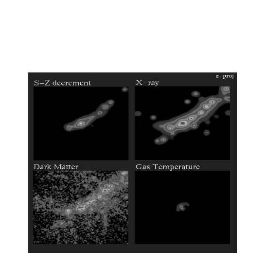
Figure 4: Views of a cluster at $z\!=\!1.24$.

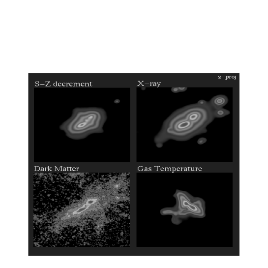
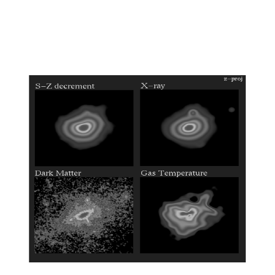
Figure 5: Views of a cluster at $z\!=\!0.6$.

Figure 6: Views of a cluster at $z\!=\!0$.

In the nearly decade since this process was first examined using self–consistent collisional gas and collisionless dark simulations matter (Evrard 1990a,b), much has changed but much has stayed the same. One of the things that has stayed the same is efficiency of thermalization of the gas, traditionally expressed as $\beta\!=\!\sigma^{2}_{1D}/(kT/\mu mp)$, the ratio of specific energies in dark matter and gas. In a comparison of twelve gas dynamics codes to the formation of a single X–ray cluster (drawn from a standard cold dark matter model with $10\%$ baryons), Frenk et al. (1998) find $\langle\beta\rangle\!=\!1.17\pm 0.06$ within $r_{200}$ to be the mean and standard deviation among the twelve codes, consistent with the value $\beta\!=\!1.2$ found by Evrard (1990a). A noteworthy point is that, despite their very different numerical treatments of shocks, codes of different type — Eulerian, Lagrangian hybrid — produced very similar values of $\beta$. A look at the P3MSPH code (Evrard 1988) solution to the comparison cluster is provided in Figures 4,  6 and  6 which show four principle cluster observables at redshifts $z\!=\!1.2,0.6$ and 0, respectively. The four panels show greyscale representations of the logarithms of the anticipated thermal Sunyaev–Zel’dovich signal (over 2 decades), intrinsic X–ray surface brightness (4 decades), gas temperature (factor 4, from $0.25-1\times 10^{8}$ K) and dark matter (DM) surface density (2.5 decades). The gas maps are smoothed on the local SPH kernel scale while the DM is left unsmoothed to show the graininess in the particle solution. A physical region of size $3.9\hbox{$\,h^{-1}$}{\rm\ Mpc}$ is shown at all redshifts. An mpeg animation of this four–panel figure is available at http://astro.physics.lsa.umich.edu/ evrard/VCL/ccp_movie.htm. There are characteristic features in these images common to all twelve codes in the comparison study. At $z\!=\!1.2$. most of the mass in the region has already collected into a long, knotty filament which will set the orientation for a chain of future merger events between the knots. One can imagine a network of such filaments covering the sky at these redshift — the “proto–cluster formation epoch”. A good portion of the absolute scale the SZ decrement shown in the figures, $3.4$ to $340\ \mu$K, is visible with current ground based techniques (e.g., Carlstrom, Joy & Grego 1996) and the cosmic web that is the large–scale distribution of clusters (Bond & Myers 1998) may be revealed by future CMB experiments. An interesting set of independently observable features occurs in a pre–merger phase displayed in Figure 6. The merger event involves a triplet, consisting of a pair of satellites (projected out along the line-of-sight in this image) each with mass in excess of $20\%$ of the dominant precursor’s mass. At the time shown, the thermalized gas envelopes of the triplet are being compressed and mildly shocked. The X–ray image displays two prominant peaks (the projected pair of satellites is to the upper right) and a strong emission weighted temperature gradient exists along the collision axis near its vertex. This pinching effect comes about because the gas at the cores of the precursors has not yet been moved off their incoming adiabats, while gas trapped near the systems center of mass is squeezed hard and subsequently strongly shocked. The hot pinched spot with adjacent sidelobes is a distinct signature of a merger occurring along the line of sight. The electron pressure visible in the SZ image has features common to both the gas density (X–ray) and temperature. Two peaks are separated by a pressure ridge of strongly shocked material perpendicular to the collision axis. Because of the confining ram pressure along the collision axis, the flow of gas at this time is highly anisotropic. Inward flow along the axis feeds outward flow off-axis, and a small fraction of gas is shed into the voids which surround the large–scale filament. The dark matter density distribution is highly flattened, with two peaks evident as in the X–ray image. Observations with the same dynamic range and resolution of these maps do not yet exist. In this sense, theory is ahead of the observation, and one can interpret these maps as predictions for upcoming, high resolution ground–based and satellite observations. The spectroscopic imaging capabilities offered by AXAF will soon begin probing the line–of–sight velocity structure, and observable velocity splittings are anticipated (Norman & Bryan 1998). Despite this seemingly active formation history, relatively little of the gas that was initially associated with the dark matter in the virial region is lost from the system at the present epoch. Figure 7 shows the normalized gas fraction $\Upsilon(r)\!=\!M_{gas}(r)/\Omega_{b}M_{tot}(r)$ evaluated within $r_{200}$ for the twelve clusters simulated in the comparison study. The solid and dashed lines show the mean and $1\sigma$ range $\langle\Upsilon\rangle\!=\!0.92\pm 0.06$ determined from the experiments. The Lagrangian codes (open symbols) seem to lose somewhat more of the gas than the other code types, but the source of this difference is not yet understood.

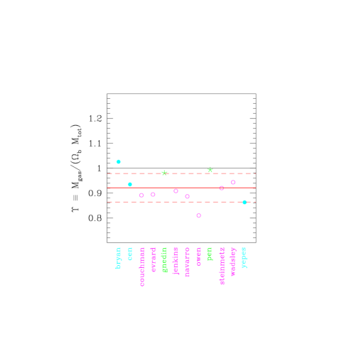
Figure 7: Normalized gas fractions within $r_{200}$ for the twelve codes in the cluster comparison study. Open symbols are Lagrangian (SPH) codes, filled circles Eulerian and stars hybrid.

Determination of the normalization of this effect is important for constraints on the total mass density $\Omega_{m}$ from the mean cluster baryon fraction (White et al. 1993; Evrard 1997). Another important factor in that argument is the normalization of the virial mass–temperature relation. Experiments show small scatter about the virial relation (Evrard, Metzler & Navarro 1996; Bryan & Norman 1998; Eke, Navarro & Frenk 1998), but the zero point remains uncertain to perhaps $15\%$. A look at the agreement between virial mass and (mass–weighted) temperature for the cluster comparison study is given in Figure 8. Hints of the overall relation $M\!\propto\!T^{2/3}$ in this diagram suggest that part of the disagreement among codes is due to a lack of strict synchronization in the cluster’s dynamical state. Small differences in the treatment of tidal fields in the linear regime, for example, can be amplified into large orbital phase differences for infalling small satellites such as that visible to the north in Figure 6. Images based on the twelve codes’ solutions exhibit noticeable differences in the positions of satellite objects.

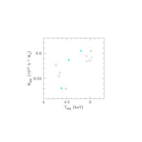
Figure 8: Temperatures and masses from the cluster comparison study. Note the $20-30\%$ range of the axes.

Table 2 summarizes the extent of the agreement among codes for internal structural properties of the cluster at the final time. The rms  deviation of spherically averaged, binned data interior to the virial radius of the cluster (using 0.2 dex binwidth) is shown. Agreement in all the listed quantities is better than $10\%$, except for the bolometric X–ray luminosity, which has an rms  of $23\%$. The luminosity $\L_{X}\!=\!\int dV\rho_{gas}^{2}(r)T^{1/2}(r)$ is particularly sensitive to the core gas structure, and the larger deviation in $L_{X}$ reflects the fact that the codes agree less well on the core structure than they do on the exterior envelope.

Table 2: Level of agreement between twelve different cosmological gas dynamics codes in the final, virial structure of a single X–ray cluster (Frenk et al. 1998).

Quantity	rms  deviation
$\rho_{DM}$	0.031
$\rho_{gas}$	0.086
$\sigma_{DM}$	0.046
$T_{gas}$	0.053
$P_{gas}$	0.081
$L_{X}$	0.23

Additional physics such as radiative cooling and magnetic fields will also affect the core structure, perhaps quite strongly. These effects are unlikely to affect the structure of the bulk of the gas in very rich clusters, but may contribute perhaps tens of percent effects. Many effects are only now being considered with careful experiments. Dolag, Bartelmann & Lesch (1998) displayed a poster at the meeting showing that the effects of magnetic fields on cluster evolution. Teyssier, Chiéze & Alimi (1997) include non–equilibrium thermodynamics and examine differences in electron and ion temperatures. Metzler & Evrard (1997) examine the effects of galactic winds. None of this additional physics appears to change the overall picture of the ICM presented above, though some details will certainly be affected. Dissenters point out that a strongly multi–phase intracluster medium is not formally ruled out (Gunn & Thomas 1996), but upcoming SZ maps combined with AXAF and XMM spectroscopic imaging will provide definitive constraints (Nagai, Sulkanen & Evrard 1998).

4 Galaxy Formation

Galaxy formation is the perennial frontier in the simulation business. As outlined in Figure 9, the radiative cooling instability within collapsed, dark matter potential wells is the essential ingredient which allows the baryons to sink to the center, become self–gravitating and, thereby, light up (White & Rees 1978). Resolving this instability is numerically challenging (see the heroic efforts of Abel, Bryan & Norman in this volume). One has the added complication that, even with a “perfect” numerical code, the physics governing star forming regions is not yet understood. The problem is formally ill–posed and solutions will be guided as much by instinct and intuition as by first principles.

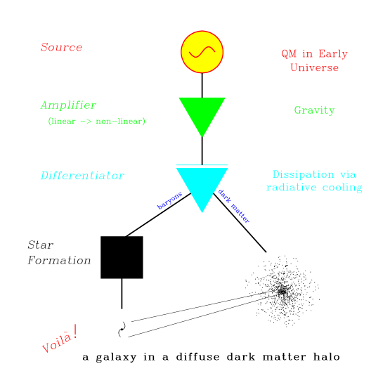
Figure 9: Flow diagram of the galaxy formation process.

Radiative cooling of the gas has been enabled in a number of calculations (Katz & Gunn 1991; Katz, Hernquist & Weinberg 1992; Evrard, Summers & Davis 1994; Navarro & White 1994; Steinmetz & Müller 1994; Frenk et al. 1996; Tissera, Lambas & Abadi 1997; Navarro & Steinmetz 1997) and a population of cold, condensed baryonic cores develops within their enveloping halos, largely along the lines scripted by the sages twenty years ago. A number of potentially interesting results have emerged, but their robustness remains in question. The issue of “biasing” — how the phase space structure of galaxies differs from that of the dark matter — is of crucial importance to interpreting data from upcoming deep optical surveys such as the Two Degree Field (2dF, see Maddox in this volume) and the Sloan Digital Sky Survey (SDSS). Biasing is a complicated issue because both gravitational (dynamical friction, merging, galaxy harassment) and non–gravitational effects (dependence of gas cooling and star formation rates on large–scale environment) may play equally important roles. Direct simulation of cluster environments (e.g., Frenk et al. 1996) in conjunction with semi–analytic approaches which postulate recipes for star formation and feedback in halos (e.g., Kauffmann, Nusser & Steinmetez 1997) are beginning to yield clues. An example of a result which may turn out to be robust is shown in Figure 10. The figure shows the pairwise peculiar velocity of galaxies and dark matter as a function of pair separation derived from a 16 million particle simulation of an LCDM universe (Pearce et al. , in preparation). Galaxies — identified with cold, high density baryonic knots in the calculation — show a lowered overall velocity distribution compared to the dark matter and this produces a much better agreement with observational values derived from the LCRS redshift survey (Lin et al. 1996). Whether or not this agreement is fortuitous hinges on the sensitivity of this result to details such as numerical parameter choices, galaxy sample definition (both real and simulated) and the weighting of the velocity statistic (Davis, Miller & White 1997). Still, the agreement between theory and observation in Figure 10 is encouraging and it may indicate that the current simulations are accurately capturing galaxy dynamics within the large–scale web of dominant dark matter.

Figure 10: Distribution of peculiar velocities for galaxies derived from a 16 million particle SPH calculation (Pearce et al. , in preparation).

5 Summary

The present state of numerical modeling of large–scale structure in the universe is
$\bullet$ well understood and ahead of observations of dark matter structure,
$\bullet$ becoming understood and on par with observations of X–ray clusters and the Ly-$\alpha$ forest,
$\bullet$ poorly understood and far behind observations of the galaxy distribution.
What does the future hold? We can expect to see parallel computers used both to expand dynamic range (by allowing bigger calculations) and also to explore model parameter space (by allowing large numbers of smaller calculations). The number and range of physical processes being included in the calculations will certainly increase. The downside of this added complexity is that it will naturally introduce additional sources for numerical error. Besides highly simplified systems, the main check on the numerical solutions may remain internal — a “galaxy comparison project” analogous to that performed for clusters is likely to occur in the near future. The upside of the added complexity is the improved contact it will bring with observational data. Spectroscopic imaging, broad band colors, kinematic studies, etc. — the sky is the target (but not necessarily the limit) in the virtual world. It is easy to foresee the problem of galaxy formation being scrutinized more thoroughly both from the “bottom–up” (via modeling of absorption line systems and high–$z$ progenitors of galaxies) and from the “top–down” (via modeling of galaxies in different large–scale environments, clusters versus the field). By attacking the problem of galaxy formation from below and above in this way, we will squeeze out the answer to the lingering question “how do galaxies trace the mass” in the universe.

References

- [1] Aarseth, S.J., Turner, E.L. & Gott, J.R. 1979, ApJ, 228, 664.
- [2] Birkinshaw, M. 1998, PhysRep, in press.
- [3] Bond, J.R. & Myers, S.T. 1996, ApjS, 103, 63.
- [4] Briel U.G., Henry J.P., Böhringer H., 1992, A&A259, L31.
- [5] Bryan, G.L. & Norman, M.L. 1998, ApJ, 495, 80.
- [6] Carlstrom, J.E., Joy, M. & Grego, L. 1996, ApJ, 456, L75.
- [7] Colberg, J.M. et al. 1998, in preparation.
- [8] Davis, M., Miller, A. & White, S.D.M. 1997, ApJ, 490, 63.
- [9] Dolag, K., Bartelmann, M. & Lesch, H. 1998, submitted to AA.
- [10] Dubinski, J. 1998, ApJ, 502, 141.
- [11] Eke, V.R., Navarro, J.F., & Frenk, C.S. 1998, ApJ, 503, 569
- [12] Evrard A.E. 1990a, ApJ, 363, 349
- [13] Evrard A.E. 1990b, in Oegerle W. R., Fitchett M. J., Danly L., eds, Clusters of Galaxies, Cambridge Univ. Press, Cambridge, p. 287.
- [14] Evrard A.E., Metzler C.A., Navarro J.F., 1996, ApJ, 469, 494.
- [15] Evrard, A.E., Summers, F.J. & Davis, M. 1994, ApJ, 422, 11.
- [16] Evrard, A.E. 1997, MNRAS, 292, 289.
- [17] Frenk, C.S. et al. 1998, submitted to ApJ.
- [18] Frenk, C.S., Evrard, A.E, White, S.D.M. & Summers, F.J. 1996, ApJ, 472, 460.
- [19] Godwin, J.G. Metcalfe, N. & Peach, J.V. 1983, MNRAS, 202, 113.
- [20] Groom, W. 1997, PhD Thesis, Cambridge University.
- [21] Jenkins, A., Frenk, C.S., Pearce, F.R., Thomas, P.A., Colberg, J.M., White, S.D.M., Couchman, H.M.P., Peacock, J.A., Efstathiou, G. & Nelson, A.H. 1998, ApJ, 499, 20.
- [22] Katz, N. & Gunn, J.E. 1991, ApJ, 377, 365.
- [23] Katz, N., Hernquist, L. & Weinberg, D.H. 1992, ApJ, 399, L109.
- [24] Kauffmann, G., Nusser, A., Steinmetz, M. 1997, MNRAS, 286, 795.
- [25] King, I. 1962, AJ, 67, 471.
- [26] Lin, H., Kirshner, R.P., Shectman, S., Landy, S.D., Oemler, A., Tucker, D.L. & Schechter, P.L. 1996, ApJ, 470, 172.
- [27] MacFarland, T. et al. 1998, in preparation.
- [28] Metzler C.A., Evrard A.E., 1997, ApJ, submitted, astro-ph/9710324.
- [29] Moore, B., Governato, F., Quinn, T., Stadel, J., Lake, G. 1998, ApJ, 499, 5.
- [30] Nagai, D., Sulkanen, M. & Evrard, A.E. 1998, submitted to MNRAS.
- [31] Navarro, J. & White, S.D.M. 1994, MNRAS, 267, 401.
- [32] Navarro, J.F. & Steinmetz, M. 1997, ApJ, 478, 13.
- [33] Norman, M.L. & Bryan, G.L. 1999, to appear in Ringberg Workshop on M87, eds. K. Meisenheimer and H-J. Roeser, Springer Verlag (astro-ph/9802335).
- [34] Stanford, S.A., Elston, R., Eisenhardt, P.R., Spinrad, H., Stern, D. & Dey, A. 1997, AJ, 114, 2232.
- [35] Steinmetz, M. & Müller, E. 1994, AA, 268, 391.
- [36] Tissera, P.B., Lambas, D.G. & Abadi, M.G. 1997, MNRAS, 286, 384.
- [37] Teyssier, R., Chièze, J.-P. & Alimi, J.-M. 1997, ApJ, 480, 36.
- [38] Tyson, J.A., Kochanski, G.P. & Dell’Antonio, I.P. 1998, ApJ, 498, L107.
- [39] White, S.D.M. & Rees, M. 1978, MNRAS, 183, 341.
- [40] White S.D.M., Navarro J.F., Evrard A.E., Frenk C.S., 1993, Nature, 366, 429