Filtration of interstellar hydrogen in the two-shock heliospheric interface: Inferences on the local interstellar electron density

Abstract

The solar system is moving through the partially ionized local interstellar cloud (LIC). The ionized matter of the LIC interacts with the expanding solar wind forming the heliospheric interface. The neutral component (interstellar atoms) penetrates through the heliospheric interface into the heliosphere, where it is measured directly “in situ” as pick-up ions and neutral atoms (and as anomalous cosmic rays) or indirectly through resonant scattering of solar Ly $\alpha$. When crossing the heliospheric interface, interstellar atoms interact with the plasma component through charge exchange. This interaction leads to changes of both neutral gas and plasma properties. The heliospheric interface is also the source of radio emissions which have been detected by the Voyager since 1983. In this paper, we have used a kinetic model of the flow of the interstellar atoms with updated values of velocity, temperature, and density of the circumsolar interstellar hydrogen and calculated how all quantities which are directly associated to the observations vary as a function of the interstellar proton number density $n_{\rm p,LIC}$. These quantities are the degree of filtration, the temperature and the velocity of the interstellar H atoms in the inner heliosphere, the distances to the bow shock (BS), heliopause, and termination shock, and the plasma frequencies in the LIC, at the BS and in the maximum compression region around the heliosphere which constitutes the “barrier” for radio waves formed in the interstellar medium. Comparing the model results with recent pickup ion data, Ly $\alpha$ measurements, and low-frequencies radio emissions, we have searched for a number density of protons in the local interstellar cloud compatible with all observations.

We find it difficult in the frame of this model without interstellar magnetic field to reconcile the distance to the shock and heliopause deduced from the time delay of the radio emissions with other diagnostics and discuss possible explanations for these discrepancies, as the existence of an additional interstellar magnetic pressure (2.1 $\mu$G $<$ B $<$ 4 $\mu$G for a perpendicular magnetic field). We also conclude that on the basis of this model the most likely value for the proton density in the local interstellar cloud is in the range 0.04 cm${}^{-3}<n_{\rm p,LIC}<$ 0.07 cm^-3.

IZMODENOV ET AL. INTERSTELLAR ATOM FILTRATION May 21, 1998 November 11, 1998 November 11, 1998 1998JA90122 AGU1999 0148-0227/99/1998JA90122$09.00 V.B. Baranov and Y.G. Malama, Institute for Problem in Mechanics, Russian Academy of Sciences, Prospekt Vernadskogo 101, Moscow, 117526, Russia. (baranov@ipmnet.ru; malama@ipmnet.ru) J. Geiss, International Space Science Institute, Hallerstrasse 6, 3012 Bern, Switzerland. (geiss@issi.unibe.ch) G.Gloeckler, Department of Physics, University of Maryland, College Park, Maryland 20742. (gloeckler@umdsp.umd.edu) V.V. Izmodenov and R. Lallement, Service d’Aeronomie du CNRS, BP 3, 91371 Verrieres le Buisson, France. (izmod@ipmnet.ru; Rosine.Lallement@aerov.jussieu.fr) To appear in the Journal of Geophysical Research, 1999.

1 International Space Science Institute, Bern, Switzerland. 2 Service d’Aeronomie, CNRS, Verrieres le Buisson, France. 3 Permanently at Department of Aeromechanics and Gasdynamics of Moscow State University, Mechanics and Mathematics faculty, Moscow, Russia. 4 Department of Physics, University of Maryland, College Park. 5 Institute for Problems in Mechanics, Russian Academy of Science, Moscow, Russia.

1 Introduction

Our solar system is moving through a partially ionized interstellar cloud. The ionized fraction of this local interstellar cloud (LIC) interacts with the expanding solar wind and forms the LIC-solar wind (SW) interface (or heliospheric interface). The characterization of this interface is a timely major objective in astrophysics and space plasma physics. The interest to the construction of the LIC/SW interaction models is increasing at the present time [Ripken and Fahr, 1983; Baranov and Malama, 1993; Zank et al., 1996; Linde et al., 1998; Pogorelov and Matsuda, 1998]. The choice of an adequate model of the interface depends on the parameters of the LIC. Some of these parameters, as the Sun/LIC relative velocity, or the LIC temperature are now well constrained [Witte et al., 1993; Lallement and Bertin, 1992; Linsky et al., 1993; Lallement et al., 1995; see, also, Frisch, 1995], but unfortunately there are no direct ways to measure the circumsolar interstellar electron (or proton) density, nor the local interstellar magnetic field, while these two parameters govern the structure and the size of our heliosphere. There have been measurements of the average electron density in the LIC toward nearby stars. However, resulting densities range from 0.05 (-0.04, +0.14) cm^-3 to up to 0.3 (-0.14, +0.3) cm^-3 depending on the ions used for the diagnostics or on which line-of-sight is probed [e.g., Lallement and Ferlet, 1997]. The most precise, temperature independent value is 0.11 cm^-3 toward the star Capella [Wood and Linsky, 1997]. In addition, what is measured is always averaged over large distances, while the ionization degree in the local interstellar medium is very likely highly variable and out of ionization equilibrium [e.g., Vallerga, 1998]. Therefore there is a need for indirect observations which can bring stringent constraints on the plasma density and on the shape and size of the interface. Such constraints should help to predict when the two Voyager spacecraft will cross the interface and whether or not they will be able to perform and transmit direct observations.

Among the various types of heliospheric interface diagnostics, there are measurements of the pick-up ions. Pick-up ions are formed when interstellar neutrals, having penetrated into the heliosphere, become ionized by charge exchange with the solar wind ions or photoionized. The newly created ions are then convected away from the Sun by the solar wind. The detection of He⁺ and He⁺⁺ provides a new determination of the neutral helium flow properties [Gloeckler et al., 1997], which can be compared with the direct detection of the neutral helium [Witte et al., 1993, 1996]. It is interesting to note that the different determinations of the helium density are now in rather good agreement. With the Solar Wind Ion Composition Spectrometer (SWICS) instrument on board Ulysses, Gloeckler et al. [1997] found $n$(HeI) = 0.0153 $\pm$ 0.0018 cm^-3 with an uncertainty of the order of only 8%, compatible with Active Magnetospheric Particle Tracer Explorers (AMPTE) results of Moebius [1996] and Ulysses Interstellar Neutral-Gas instrument (GAS) results of Witte et al. [1996]. As for hydrogen, the first successful detection of H⁺ pick-up ions has been done with the SWICS instrument on board the Ulysses spacecraft [Gloeckler et al., 1993]. From the H⁺ fluxes, one can infer a new value for the neutral hydrogen flux in the inner heliosphere. Indeed, Gloeckler et al. [1997] used the pick-up ions data to infer the interstellar hydrogen atom number density in the outer heliosphere and found $n(\textnormal{HI})=0.115\pm 0.025$ cm^-3 with an uncertainty of 20%. Note that in all these works the H and He number densities are obtained using the classical so-called “hot” model of interstellar neutrals flow in the heliosphere. The H number density obtained from pickup ion measurements is close to the lower range of the interval derived from optical resonance data revised by Quémerais et al. [1996], i.e., 0.11-0.17 cm^-3.

The neutral H density in the inner heliosphere is dependent on the perturbations the neutral H suffers at the heliospheric interface. Since interstellar helium is not depleted in the heliospheric interface region (n(He) heliospheric $\approx$ n(He) interstellar), it is possible to compare the properties of the neutral hydrogen and helium flows. Taking into account the newly derived neutral hydrogen to neutral helium ratio in the LIC [Dupuis et al., 1995]

$$\frac{n_{\rm LIC}\textnormal{(HI)}}{n_{\rm LIC}\textnormal{(HeI)}}=14\pm 1$$

Lallement [1996] related the neutral H density in the heliosphere to the plasma density in the LIC, using a proxy for the filtration ratio of H as a function of the plasma density. The proxy was derived from Baranov and Malama [1993] model filtration ratios. It was found that if n(H) in the inner heliosphere is of the order of 0.15 (0.10, respectively) cm^-3, then the electron density in the circumsolar medium is close to 0.05 (0.11, respectively) cm^-3. Gloeckler et al. [1997], using the new SWICS pick-up ions results and an interstellar HI/HeI ratio of $13\pm 1$ (the average value of the ratio toward the nearby white dwarfs), concluded that $n_{\rm LIC}(\textnormal{HI})=0.2\pm 0.03$ cm^-3, which corresponds to a filtration factor (the ratio of atom number density in the outer heliosphere to atom number density in the LIC)

$$\chi=\frac{n_{\rm TS}({\rm HI})}{n_{\rm LIC}({\rm HI})}=0.58\pm 0.15$$ (1)

where subscript TS is termination shock. Then, on the basis of estimates of the charge-exchange processes, they obtained for the interstellar proton (or electron) number density $n_{\rm p,LIC}=0.04\pm 0.017$ cm^-3.

For a given plasma density, there is a nonnegligible influence of the neutral density in the LIC on the filtration ratio. The filtration ratios used by Lallement [1996] were taken from a model with $n_{\rm LIC}({\rm HI})=0.14$ cm^-3 [Baranov and Malama, 1993], introducing some unconsistency in the method. In what follows, we will make use of the more appropriate value $n_{\rm LIC}({\rm HI})=0.2$ cm^-3, which is based on the well-measured neutral helium density and the interstellar ratio measured with the Extreme Ultraviolet Explorer (EUVE).

The goal of this paper is to determine a range for the interstellar proton number density $n_{\rm p,LIC}$ that is compatible with all observations, using the two-shock heliospheric interface model of Baranov and Malama [1993, 1995, 1996] for the updated value $n_{\rm LIC}({\rm HI})=0.2$ cm^-3. The observations we will consider are, in addition to the pick-up ions quoted above, the temperature and velocity of the neutral H flow in the inner heliosphere and the Voyager radio emissions. Recently, Linsky and Wood [1996] have detected the heated and decelerated gas from the so-called H wall corresponding to the compressed region between the bow shock (BS) and the heliopause (HP), in absorption toward the star $\alpha$ Centauri. Gayley et al. [1997] have compared the observed absorption with the theoretical absorption for three different models. One of these models is a two-shock model, and the two other correspond to the “subsonic” case; That is, they have modified the equation of state of the gas to simulate the effect of an interstellar magnetic field. These authors conclude that the H wall absorption favors the “subsonic case.” We have not included such diagnostic in our study for the following reasons: in our “supersonic” case, the simulations show that it is hard to distinguish H walls built up for $n_{\rm p,LIC}=0.04$ cm^-3 or for 0.2 cm^-3. As a matter of fact, if $n_{\rm p,LIC}$ increases, the gas is more heated and compressed, but the thickness of the H wall is reduced. Also, the precision required to model the differences between the theoretical absorptions, namely small differences of the order of a few kilometers per second at the bottom of the lines, is of the order of the differences between the model results from different groups for the same parameters in the supersonic case [see Williams et al., 1997, Appendix B]. A larger difference may exist between the “supersonic” and the “subsonic” cases, large enough to favor the subsonic case, as argued by Gayley et al. Our approach is to use other independent diagnostics, namely all heliospheric data, in order to constrain the requirements for additional physics.

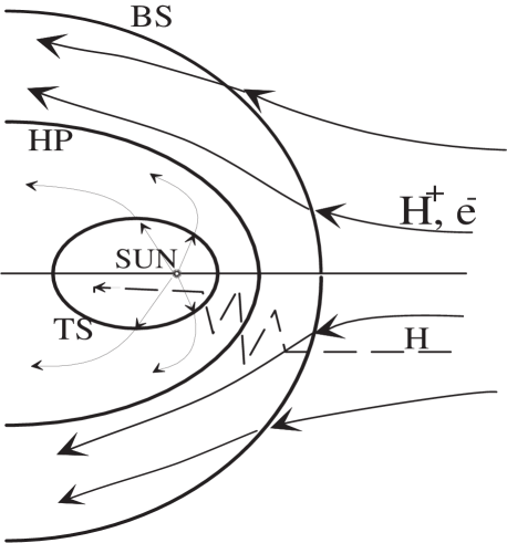
Figure 1: Qualitative picture of the solar wind interaction with
the local interstellar medium (LISM). Here BS is the bow shock,
HP is the heliopause, and TS is the termination shock.

The model is a self-consistent gasdynamic-kinetic model of the solar wind interaction with the local interstellar medium, which takes into account the mutual influence of the plasma component of the LIC and interstellar H atoms in the approximation of axial symmetry (Figure 1).

Then we compare the range of $n_{\rm p,LIC}$ values derived from the pick-up measurements with the range that is compatible with observations of the backscattered solar Ly $\alpha$ emission as well as from the interpretation of the 2-3 kHz emission recorded by the Voyager radio instruments. As a tool for the analysis of future measurements, we also calculate the relevant observational parameters as a function of the interstellar plasma density.

2 Formulation of the Problem

The interface is characterized by three surfaces: the solar wind termination shock (TS), the heliopause, and the interstellar bow shock. The interstellar atom flow in the heliospheric interface must be described kinetically because the mean free path of the neutral atoms is of the order of the size of the heliospheric interface. In fact, Baranov et al. [1998] have shown kinetic and hydrodynamic models of the interstellar atom flow may give significant differences. In order to obtain the kinetic distribution function, the Boltzman equation must be solved:

$$\vec{w_{\rm H}}\frac{\partial f_{\rm H}(\vec{r},\vec{w}_{\rm H})}{\partial\vec{r}}+\frac{F}{m_{\rm H}}\frac{\partial f_{\rm H}(\vec{r},\vec{w}_{\rm H})}{\partial\vec{w}_{\rm H}}=$$

$$-f_{\rm H}(\vec{r},\vec{w}_{\rm H})\int|\vec{w}_{\rm H}-\vec{w}_{\rm p}|\sigma^{\rm HP}_{ex}f_{\rm p}(\vec{r},\vec{w}_{\rm p})d\vec{w}_{\rm p}$$ (2)

$$+f_{\rm p}(\vec{r},\vec{w_{\rm H}})\int|\vec{w}_{\rm H^{*}}-\vec{w}_{\rm H}|\sigma^{\rm HP}_{ex}f_{\rm p}(\vec{r},\vec{w}_{\rm H^{*}})d\vec{w}_{\rm H^{*}}$$

$$-(\beta_{i}+\beta_{\rm impact})f_{\rm H}(\vec{r},\vec{w}_{\rm H})$$

Here $f_{\rm H}(\vec{r},\vec{w}_{\rm H})$ is distribution function of the H atoms, $f_{\rm p}(\vec{r},\vec{w}_{\rm p})$ is the local distribution function of the protons which is assumed to be Maxwellian, $\vec{w}_{\rm p}$ and $\vec{w}_{\rm H}$ are the individual proton and H atom velocities, respectively. Here $\sigma^{\rm HP}_{ex}$ is the charge exchange cross section of an H atom with a proton, $\beta_{i}$ is the photoionization rate, $m_{\rm H}$ is the mass of atom, $\beta_{\rm impact}$ is the electron impact ionization rate, and $F$ is the sum of solar gravitational force and solar radiation pressure force.

Equation (2) takes into account the following processes.

1.The resonance charge exchange process:

$$\textnormal{H + H}^{+}\leftrightarrow\textnormal{H}^{+}+\textnormal{H}$$

with charge exchange cross section [Maher and Tinsley, 1977] $\sigma^{\rm HP}_{ex}=10^{-14}$ (1.64 - 0.0695 ln V)², cm². Here V is the relative velocity measured in centimeters per second.

2. The photoionization process: The photoionization rate is

$$\beta^{\rm H}_{i}=\beta^{\rm H}_{ph,E}\lgroup\frac{r_{e}}{r}\rgroup^{2},\beta^{\rm H}_{ph,E}=8.8\cdot 10^{-8}\>\textnormal{s}^{-1}$$

where $\beta^{\rm H}_{ph,E}$ is the photoionization rate at the Earth’s orbit and $r_{e}$ is 1 AU.

3. The electron impact ionization process: The rate is given by [Lotz, 1967]

$$\beta_{e}=\frac{2}{P_{1}}\sqrt{\frac{2}{P_{1}m_{e}\pi}}a\sqrt{\lambda}\{E_{1}(\lambda)$$ (3)

$$-b\cdot e^{c}\frac{\lambda}{\lambda+c}E_{1}(\lambda+c)\}$$

Here $\lambda=\frac{P_{1}}{kT_{e}}$, $E_{1}(\lambda)=\int^{\infty}_{1}\frac{e^{(}-\lambda t)}{t}dt$. The values $P_{1},a,b,c$ are equal to $P_{1}=13.6$ eV, $a=4.\cdot 10^{-14}$ cm² eV², b=0.6, c=0.56.

4. The solar gravitation ($F_{g}$) and solar radiation pressure ( $F_{r}$ )processes:

$$F=F_{g}-F_{r}=(1-\mu)F_{g},\mu=F_{r}/F_{g}$$

We have used the value $\mu=0.8$. Most of our results are independent of the chosen value, since $F$ has a nonnegligible influence only within a few AU from the Sun.

The difficulty with modeling the H atom flow lies in the necessity to take into account the mutual influence of the atomic and plasma components [Baranov and Malama, 1993, 1995, 1996] and to solve the kinetic equation (2) together with hydrodynamic equations for the plasma component. To calculate the H atom flow, we used the axisymmetric model and the method developed by Malama [1991] and Baranov and Malama [1993, 1995, 1996]. The boundary conditions for the proton density, the bulk velocity and the Mach number of the solar wind at the Earth’s orbit are taken as $n_{{\rm p},E}=7.00$ cm^-3, V${}_{E}=450$ km s^-1, M_E=10.

In the unperturbed LIC, we use $V_{\rm LIC}=25$ km s^-1 and $T_{\rm LIC}=5600$ K for all sets of model parameters. These values are close to the most recent determinations of interstellar He parameters obtained by Witte et al. [1996] with the GAS instrument on Ulysses. These authors give an interstellar helium velocity $24.6\pm 1.1$ km s^-1 and a helium temperature of $5800\pm 700$ K. The H atom number density is kept fixed at $n_{\rm H,LIC}=0.2$ cm^-3, as discussed in the introduction. This value corresponds to the mean value given by Gloeckler et al. [1997]. For our calculations we have chosen the following values of proton number density: $n_{\rm p,LIC}=0.3,0.2,0.1,0.07,0.04$ cm^-3.

3 Results of Modeling Calculations

Using the heliospheric interface model with the solar wind and LIC parameters described above, we have calculated the structure of the heliospheric interface (positions and shapes of the TS, HP, and BS) and the distributions of plasma and neutral components. The distributions of the plasma and of the different H atom populations as well as the influence of the different physical processes have been discussed by Baranov and Malama [1993, 1995, 1996] and Baranov et al. [1998]. Here we present and discuss only selected results of our calculations, which will be useful for analyses of interstellar proton number density in the section 4. Figure 2 shows the BS, HP,and TS distances to the Sun in the upwind direction as a function of the interstellar proton number density. It can be seen from the figure that the BS has the largest response to the interstellar proton density variations. As a matter of fact, the distance to the BS in the upwind direction decreases from 360 AU (for $n_{\rm p,LIC}=0.04$ cm^-3) to 180 AU (for $n_{\rm p,LIC}=0.3$ cm^-3), whereas the distance to the heliopause varies from 185 to 110 AU. Thus the heliospheric interface region (the region between the BS and TS) becomes narrower while the interstellar proton number density is increased. The distance to the termination shock is NOT very sensitive to the proton density (between $\approx$ 100 and $\approx$ 70 AU). The inferred range is compatible with the shock location deduced from the radial gradients of the ACR energy spectra [e.g. Cummings and Stone, 1996].

Figure 2: Positions of the bow shock, the heliopause and the
termination shock in upwind direction as a function of interstellar
proton number density.

Figure 3: The number density of interstellar atoms as a function
of heliospheric distance for different values of interstellar proton
number density.

Figure 3 shows the number density of interstellar H atoms as a function of the heliocentric distance in the upwind direction. As the proton number density increases, the hydrogen wall between the BS and the HP becomes “higher.” The filtration factor (defined in equation (1)) decreases. Indeed, an increase of the proton number density in the LIC leads to increase of the proton number density between the BS and the HP and to an increase of the secondary H atoms number density resulting from the charge-exchange between primary interstellar H atoms and decelerated protons. This population of secondary H atoms has a smaller bulk velocity and a higher temperature than the primary interstellar H atom population. It is the increase of the number density of the secondary H atoms which reinforces the H wall and decreases the filtration factor. Figure 3 also shows that filtration occurs mainly in the region between the BS and the HP.

Table 1 shows how the number density of primary interstellar and secondary H atoms at the termination shock in the upwind direction changes as a function of the density $n_{\rm p,LIC}$. For $n_{\rm p,LIC}=0.04$ cm^-3, primary interstellar H atoms represent about 50% of the H atoms entering the heliospheric interface, while for $n_{\rm p,LIC}=0.2$ cm^-3, they represent only 6% of the total. Since the secondary H atoms have a smaller velocity and a higher temperature than the primary interstellar atoms [cf., Baranov et al., 1998], the bulk velocity and the temperature of the mixed H atom gas vary with the interstellar proton number density (Table 1). For example, for $n_{\rm p,LIC}=0.04$ cm^-3, the temperature and the velocity are $T_{\rm H,TS}=10500$ K and $V_{\rm H,TS}=22.5$ km s^-1, while for $n_{\rm p,LIC}=0.3$ cm^-3, the values are $T_{\rm H,TS}=14000$ K and $V_{\rm H,TS}=17.0$ km s^-1.

Figure 4: (a) Number density, (b) the velocity, and (c) the tem-
perature of intertellar atoms at the termination shock in upwind di -
rection as functions of interstellar proton number density.

Figures 4 shows the interstellar atom density, velocity, and temperature at the termination shock in the upwind direction as a function of $n_{\rm p,LIC}$. It can be seen from the figure that the interstellar atom number density and the filtration factor decrease rapidly when the proton number density is increased from 0 to 0.04 cm^-3 and much less rapidly for higher $n_{\rm p,LIC}$ values. As a consequence, small uncertainties in the atom density at the TS will give us small uncertainties in $n_{\rm p,LIC}$ for $n_{\rm p,LIC}<0.04$ cm^-3 (“low density case”) and relatively large ones for, say, $n_{\rm p,LIC}>0.07$ cm^-3 (“high density case”). The same situation occurs for the temperature (Figure 4c), showing that its determination is an excellent diagnostic in the low density case. Contrary the filtration factor and temperature, the velocity dependence on $n_{\rm p,LIC}$ (Figure 4b) remains about the same for the full range 0 cm${}^{-3}<n_{\rm p,LIC}<0.3$ cm^-3, showing that knowledge of $V_{\rm H,TS}$ is very helpful for determining $n_{\rm p,LIC}$ even in the “high density case” (as long as $n_{\rm p,LIC}<0.2$ cm^-3).

Figure 5 shows the plasma frequency in the interstellar plasma and at the bow shock on the upwind axis as a function of the proton density. These frequencies may be important if, as it has been suggested by Gurnett et al. [1993], the 1.8 kHz emission cutoff corresponds to the interstellar plasma frequency, and if, as suggested by Grzedzielski and Lallement [1996], the 2 kHz band was emitted in the compression region ahead of the bow shock. Also plotted is the frequency corresponding to the maximum plasma density along the upwind and crosswind axis (the “pile-up” region), which according to the present model occurs between the BS and the HP. This may be an important parameter too, since, according to the above scenario this is the “obstacle” the 2 kHz signal has to overcome to be able to enter the heliosphere.

Recently, Linsky and Wood [1996] have convincingly shown that the excess of neutral hydrogen absorption seen in the spectrum of the star $\alpha$ Centauri had indeed its origin in the heated and decelerated gas from the so-called H wall corresponding to the compressed region between the BS and the HP. While being an important discovery, simulations show it is hard to distinguish from these observations between the H walls built up for $n_{\rm p,LIC}=0.04$ or 0.2 cm^-3. As a matter of fact , if $n_{\rm p,LIC}$ increases, the gas is more heated and compressed, but the thickness of the H wall is reduced. This is why we have not included the H wall absorption in this parametric study. A somewhat larger difference does exist between the “supersonic” and “subsonic” cases, as calculated by Gayley et al. Here we consider the supersonic case only.

Figure 5: The plasma frequencies in the interstellar plasma
(solid curve 1), at the bow shock (curves 2 and 3), and in the ma-
ximum plasma density region between BS and HP (curves 4 and 5)
as functions of interstellar proton number density. Dotted curves
3 and 5 correspond to upwind, dashed curves 2 and 4 correspond
to crosswind.

4 The Influence of the Interstellar Proton Number Density

4.1 The Neutral Hydrogen Density in the Inner Heliosphere

The pick-up ions measurements provide a determination of the neutral H flux which has the advantage of being dependent on the solar ionization processes only. The situation is even better since the solar wind measured at the same time as each set of pick-ups has indeed been the main ionizing agent of these particular pick-ups. At variance with the pick-ups, the use of the backscattered Ly $\alpha$ glow as a neutral H density diagnostic suffers from uncertainties on photon radiative transfer effects and on radiation pressure and ionization rate measurements [see, e.g., Quémerais et al., 1994].

As mentioned above, Gloeckler et al. [1997] have obtained from the SWICS Ulysses pick-up ion measurements for the neutral hydrogen number density at the termination shock

$$0.09\>\textnormal{cm}^{-3}<n_{\rm H,TS}<0.14\>\textnormal{cm}^{-3}$$ (4)

using the classical “hot” model. Because the “hot” model does not take into account any heliospheric filtering at the interface, it is reasonable to assume that this measured value corresponds to interstellar atom number density at the TS. Comparing this with the results of our numerical calculations (Figure 4a), we obtain

$$0.02\>\textnormal{cm}^{-3}<n_{\rm p,LIC}<0.1\>\textnormal{cm}^{-3}$$ (5)

crrrrrrrrrrr Interstellar Atoms Number Density at the Termination Shock ($n_{\rm H,LIC}=0.2$ cm${}^{-3})$ 1 $n_{\rm p,LIC}$, cm^-3 & $n_{\rm prim,TS}$, cm^-3 $n_{\rm sec,TS}$, cm^-3 $n_{\rm H,TS}$, cm^-3 $V_{\rm H,TS}$, km s^-1 $T_{\rm H,TS}$, K

0.3 & 0.07 17 14000 0.2 0.0045 0.075 0.0795 18 13500 0.1 0.02 0.07 0.09 20 12500 0.07 0.03 0.065 0.095 21 12000 0.04 0.055 0.05 0.105 22.5 10500

llll 41pc Intervals of Possible Interstellar Proton Number Densities 2 Type of Heliospheric Interface Diagnostics & Range of Interstellar Proton Number Density

SWICS/Ulysses pick-up ion &    0.09 cm${}^{-3}<n_{\rm H,TS}<0.14$ cm^-3 0.02 cm${}^{-3}<n_{\rm p,LIC}<0.1$ cm^-3    Gloeckler et al., [1997] Ly- $\alpha$, intensity    0.11 cm${}^{-3}<n_{H,TS}<0.17$ cm^-3 $n_{\rm p,LIC}<0.04$ cm^-3 or    Quémerais et al., [1994] $n_{\rm p,LIC}<0.07$ cm^-3 (for $n_{\rm H,LIC}=0.23$ cm^-3 ) Ly-$\alpha$, Doppler shift    18 km s${}^{-1}<V_{H,TS}<21$ km s^-1 0.07 cm${}^{-3}<n_{\rm p,LIC}<0.2$ cm^-3    Bertaux et al. [1985], Lallement et al.,    [1996], Clarke et al. [1998] Voyager kHz emission (events)    110 AU $<R_{\rm AU}<$ 160 AU 0.08 cm${}^{-3}<n_{\rm p,LIC}<0.22$ cm^-3    Gurnett and Kurth [1996] Voyager kHz emission (cutoff)    1.8 kHz $n_{\rm p,LIC}=0.04$ cm^-3    Gurnett et al. [1993], Grzedzielski and    Lallement [1996] See, also, table 2. The lower value of the neutral density interval falls within the insensitive part (“high density case”) of the function $n_{\rm H,TS}(n_{\rm p,LIC})$ in figure 4a, and this explains the large range resulting for $n_{\rm p,LIC}$. This is something only estimates as those from Gloeckler et al. [1997] do not show and the present work makes visible. The mean Gloeckler et al. value $n_{\rm H,TS}=0.115$ cm^-3 ($n_{\rm H,TS}/n_{\rm H,LIC}=0.575$) corresponds here to $n_{\rm p,LIC}=0.03$ cm^-3. This value is slightly lower than the one obtained by Gloeckler et al. In order to narrow the range for the interstellar proton density on the basis of pick-up measurements, we need a larger precision on the neutral H density. As we mentioned above, the backscattered solar Ly $\alpha$ intensity can also provide an estimate of the interstellar atom number density. A compilation and reinterpretation of many previous determinations of the H atom density by Ly $\alpha$ measurements has been done by Quémerais et al. [1994]. The resulting density is in the range of 0.11 cm^-3 - 0.17 cm^-3, corresponding to

$$n_{\rm p,LIC}<0.04\>\textnormal{cm}^{-3}$$ (6)

The range obtained by Quémerais et al. includes the mean value of the $n_{\rm p,LIC}$ determination by Gloeckler et al.

4.2 Velocity and Temperature

Figure 4 shows that the temperature and the velocity of the H atoms in the heliosphere depend rather strongly on the LIC proton number density. These model predictions can be compared with estimations obtained from measurements of the backscattered solar Ly $\alpha$ radiation. Velocities are deduced from Doppler shifts, while temperatures are deduced from linewidths with the help of flow modeling. However, one has to overcome two difficulties:
(1) The velocity determination suffers from uncertainties in the radiation pressure. Depending on the balance between radiation pressure and gravitation, the velocity of the gas close to the Sun increases ($\mu<1$ valid for low activity) or decreases ($\mu>1$ valid for high activity). Therefore an uncertainty in the balance parameter $\mu$ introduces an error in the H velocity far from the Sun. (2) The temperature determination suffers from uncertainties on the radiative transfer effects, which broaden the lines in a manner that is not yet satisfyingly represented.

Measurements of the interplanetary Ly $\alpha$ emission line profile obtained with a hydrogen absorption cell on board Prognoz 5/6 [Lallement et al., 1984; Bertaux et al., 1985] have yielded a good estimate of the bulk velocity ($20\pm 1$ km s^-1). In this case, $\mu$ was determined by adjustment of the model. However, the “hot” model never reproduced the data in all directions simultaneously. More recently, Ly $\alpha$ spectral measurements [Lallement et al., 1996, Clarke et al., 1998] confirmed that the inflow speed of H atoms far from the Sun (at the TS) is within the range of 18 - 21 km s^-1 using estimates of $\mu$ based on solar Ly $\alpha$ measurements corresponding to the periods of observation.

According to the results of our calculations (Figure 4b), the velocity interval 18 km s${}^{-1}<V_{\rm H,TS}<21$ km s^-1 corresponds to the range

$$0.07\>{\rm cm}^{-3}<n_{\rm p,LIC}<0.2\>{\rm cm}^{-3}$$ (7)

The analysis of the Prognoz 5/6 H cell data also provided the “line profile” temperature (8000 $\pm$ 1000 K) of the H atoms in the inner heliosphere. This is about 1500-2500 K above the helium temperature. However, it is important to note that only line-profiles observed in the direction perpendicular to the main flow could be used and traced back through modeling to the temperature “at infinity,” i.e., before the interaction with the Sun (but still inside the heliospheric interface). In addition to the uncertainties on the effect of radiative transfer on line profiles, this determination may have been slightly biased by the assumption of a given temperature in the absorption cell and the temperature slightly underestimated. Now, the Hubble Space Telescope Ly $\alpha$ spectral observations mentioned above have shown that the line profiles on the upwind and downwind side are much larger than what predict classical models for a gas initially at the same temperature as helium. Inferred line-of-sight temperatures are as high as 15,000-20,000 K [Clarke et al., 1998]. This is in favor of a nonnegligible heating of hydrogen at the interface. Still, the role of radiative transfer has to be assessed before one can derive a confidence interval for the kinetic temperature.

4.3 Heliospheric Radio Emissions

The radio emission detected by Voyager 1 and 2 spacecraft is another type of heliospheric interface diagnostics. It is believed that the emission region is connected with the vicinity of the heliopause. Major events of kilohertz emission observed in 1983-1984 and in 1992-1993 were associated with intense solar wind solar events in 1982 and 1991. The propagation delay in both cases is about 400 days. Using measurements of the propagation speed of the interplanetary shocks produced by these events and the time delay of the onset of the radio burst, Gurnett and Kurth [1996] could estimate the distance to the heliopause and found that it ranges from 110 to 160 AU. The comparison with our calculations (Figure 2) shows that this range for the HP location (for the upwind side) corresponds to an interstellar proton number density

$$0.08\>\textnormal{cm}^{-3}<n_{\rm p,LIC}<0.22\>\textnormal{cm}^{-3}$$ (8)

The second feature is the lower frequency (1.8-2.1 kHz) emission band and in particular the well-defined “cutoff” of this emission at 1.8 kHz. This sharp “cutoff” could be related to the LIC density, which is the unique constant parameter for the whole interface. The plasma frequency at 1.8 kHz implies an interstellar electron density of 0.04 cm^-3. As explained in the previous section, any radiation emitted in the interstellar medium is, in principle, prevented to enter the interface due to a maximum compression region characterized by a density we have represented in Figure 5. Despite these difficulties, it remains that there is no other explanation for the cutoff, and the particular value $n_{\rm p,LIC}=0.04$ cm^-3 has a high probability of being the true circumsolar interstellar density.

4.4 A Synthesis?

It can be seen from equations (6) and (7) that there is already a small discrepancy between the interstellar plasma densities obtained from Ly $\alpha$ intensity measurements and the Ly $\alpha$ profile (Doppler’s shift) measurements. At the same time, both intervals have an intersection with the interval in equation (5) derived from pick-up ions measurements. This discrepancy disappears if both the interstellar proton and neutral number densities are higher than the values we have assumed. In this case, it is possible to have simultaneously a smaller bulk velocity and a higher neutral H density in the heliosphere. However, there is a model-independent limit on the LIC H atom density from the relative H/He abundance $n_{\rm H,LIC}<0.23$ cm^-3 (see section 1). This implies that only a small increase of $n_{\rm H,LIC}$ (and then of $n_{\rm p,LIC}$) is relevant. For the maximum value $n_{\rm H,LIC}=0.23$ cm^-3 and $n_{{\rm p,LIC}}=0.07$ cm^-3 (in agreement with equation (5)), we find $n_{\rm H,TS}=0.11$ cm^-3, assuming the same filtration factor as for $n_{\rm H,LIC}=0.20$ cm^-3 and $n_{\rm p,LIC}=0.07$ cm^-3. This value corresponds to lower limit derived from Ly $\alpha$ intensity measurements.

Up to now, we can conclude that the pair of values $n_{\rm H,LIC}=0.23$ cm^-3 and $n_{\rm p,LIC}=0.07$ cm^-3 is in agreement with both observations of pick-up ions and Ly $\alpha$ radiation. Now, we note that $n_{\rm p,LIC}=0.07$ cm^-3 is very close to the lower limit in equation (8). Considering that the source of the 3 kHz emission may not be exactly at the HP but in the region between the TS and the HP could help to reconcile the two results. This could be due to, for example, the influence of the electron impact ionization on the plasma flow in the region between the TS and the HP. As a matter of fact, this process leads to a strong plasma density gradient between the HP and the TS.

However, in any case, the above values are not compatible with the 1.8 kHz cutoff, if it corresponds to the interstellar emission. If we assume now that this is really the case, then we have to explain why equations (6) and (8) are not justified.

We can give two possible explanations for the discrepancy with equation (8). First, it is possible that the source of the emission is not exactly at the HP but in the region between the TS and the HP, as it was mentioned above. A second possible explanation is that there is some additional pressure in the interstellar medium. It may be a magnetic field pressure [Myasnikov, 1997; Linde et al., 1998; Pogorelov and Matsuda, 1998] or a low energy cosmic ray pressure [Izmodenov, 1997; Myasnikov et al., 1997]. Owing to this additional pressure, the HP would be closer to the Sun as compared with what the present model implies for $n_{\rm p,LIC}$ as low as 0.04 cm^-3.

The calculation of the interstellar magnetic field (IMF) strength required to push the HP as close as 110-160 AU requires a full MHD model coupled to a neutral flow model. Such a model is not yet available. The magnetic field is taken into account in some gasdynamical models by modifying the equation of state for the plasma [e.g., Gayley et al., 1997], which is appropriate in some specific conditions of orientation and Mach numbers. MHD models have been built but without inclusion of the coupling to the neutral flow. Hereafter, we estimate the IMF strength needed to reconcile $n_{\rm H,LIC}=0.04$ cm^-3, connected with the 1.8 kHz cutoff, and HP distance measurements by Gurnett and Kurth [1996]. We use the following formula deduced from our calculations and Figure 2 in the absence of magnetic and cosmic rays pressure:

$$R_{\rm HP}=24(3.6-P_{\rm LIC}\cdot 10^{12})+110$$ (9)

Here $R_{\rm HP}$ is the distance to the heliopause (upwind direction) in astronomical units, $P_{\rm LIC}$ is the interstellar pressure in dyn cm^-2 deduced from our parameters. We then replace $P_{\rm LIC}$ by the more general term

$$P_{\rm LIC}=n_{\rm p,LIC}\cdot(2k_{b}T_{\rm LIC}+m_{\rm H}V^{2}_{\rm LIC})$$ (10)

$$+\alpha\frac{B^{2}_{\rm LIC}}{8\pi}+P_{\rm GCR,LIC}$$

where $n_{\rm p,LIC}$, $T_{\rm LIC}$,and $V_{\rm LIC}$ are interstellar proton number density, temperature, and velocity, respectively, $B_{\rm LIC}$ is the interstellar magnetic field strength, $\alpha$ is an amplification factor ($\alpha\approx 0-4$) determined by the angle between the interstellar magnetic field and velocity vector [Holtzer, 1989; see, also, Frisch, 1993], and $P_{\rm GCR,LIC}$ is galactic cosmic ray pressure.

By doing so, we assume that an additional nongasdynamical pressure acts on the shape of the heliopause on the same way as a gasdynamical (proton and electron) pressure. The influence of interstellar atoms is included in the numerical coefficients of equation (9), which implies this formula is valid only if $n_{\rm H,LIC}$ is of the order of 0.20 cm^-3.

It is interesting to note that if the direction of the interstellar magnetic field is the same as the wind direction (in principle the unique possibility for a two-dimensioned modeling), the heliocentric distance of the heliopause increases as a result of the magnetic field tension [Baranov and Zaitsev, 1995] along the wind axis, whereas this distance decreases in the wing due to magnetic field pressure. In this case, the formula (9) does not work. However, the parallel IMF is probably unlikely because, to reconcile data, we need the heliopause closer to the Sun.

Our formula (9) probably gives better estimates of the HP distance variation as a function of the interstellar pressure than estimates based on balance between the solar and interstellar pressures [see, e.g., Holtzer, 1989], because we take into account the plasma compressibility and the influence of interstellar neutrals on the plasma structure. Actually, owing to these effects, the heliospheric interface is a kind of damping region for any changes in the interstellar pressure. Using balance pressure only, one overestimates the variation of the HP distance due to interstellar pressure.

If we assume that $n_{\rm p,LIC}=0.04$ cm^-3 and that the GCR pressure is $P_{\rm GCR}=0.3\cdot 10^{-12}$ dyn cm^-2 [Holtzer, 1989], we find from equation (9) that the interval 110 AU $<R_{\rm HP}<$ 160 AU [Gurnett and Kurth, 1996] corresponds to

$$0.737\cdot 10^{-12}\>{\rm dyn\>cm^{-2}}<\alpha\frac{B^{2}}{8\pi}<2.82\cdot 10^{-12}\>{\rm dyn\>cm^{-2}}$$

For $\alpha$=4 (perpendicular magnetic field) [Holtzer, 1989],

$$2.1\>\mu{\rm G}<B<4\>\mu{\rm G}.$$

This interval is in agreement with the current estimates of the interstellar magnetic field strength [e.g., Frisch, 1995]. However, it is necessary to note that if indeed the IMF strength is above 2.1 $\mu$G, then a full “subalfvenic” model is required. However, in the subalfvenic case, there is no bow shock and then, to date, no explanation for the 2 kHz radio emission.

It remains that despite the addition of such a pressure, the discrepancy with the bulk velocity measurements equation (6) still remains. If $n_{\rm p,LIC}=0.04$ cm^-3, then the bulk velocity is $V_{\rm H,TS}=22.5$ km s^-1 (23 km s^-1 for an interstellar velocity of 25.5 km s^-1). As we already discussed, the Doppler shift measurements are sensitive to the Ly $\alpha$ radiation pressure. The above value of the bulk velocity implies that the radiation pressure is above what has been inferred from the H cell data (there is less deceleration induced by the interface and more due to the radiation pressure).

All the above estimates have been done by implicitely assuming that the additional pressure due to the fraction of neutral gas coupled to the plasma remains of the same order with and without interstellar magnetic field. Of course, both the intensity and the direction of the magnetic field change the plasma pressure between the bow shock and the heliopause, but they also change the thickness of this region. An increase of the plasma compression in all cases corresponds to a decrease of the thickness; That is, the two phenomena tend to compensate, as it can be seen in the results of Linde et al. [1998] and Baranov and Zaitsev [1995], for direction and intensity changes, respectively. The filtering depends on the product of plasma density and thickness, and, as a consequence, it should not change dramatically. More accurate computations on the basis of MHD models are needed to quantify such changes.

5 Conclusions

We have performed a parametric study which shows how sensitive and compatible are the various types of diagnostics of the interstellar plasma density $n_{\rm p,LIC}$, i.e., the interstellar neutrals temperature, number density and velocity, and the radio emissions time delays and frequency ranges. For the neutrals, there are two regimes: For low values ($n_{\rm p,LIC}<0.05$ cm^-3), the most sensitive parameters are the neutral H density and temperature in the inner heliosphere, while for higher values, the H bulk velocity only remains sensitive.

In the light of this study, we have discussed the observational results. Our main conclusion is that it is impossible to reconcile the results obtained from all types of data as they stand now. There is a need for some modifications of the interpretations or the confidence intervals. Two types of solutions (which are mutually exclusive) seem to be favored: (1) It is possible to reconcile the pick-up ions and Ly $\alpha$ measurements with the radio emission time delays if a small additional interstellar (magnetic or low energy cosmic ray) pressure is added to the main plasma pressure. In this case, $n_{\rm p,LIC}=0.07$ cm^-3 and $n_{\rm H,LIC}=0.23$ cm^-3 is the favored pair of interstellar densities. However, in this case, the low frequency cutoff at 1.8 kHz of course cannot be connected to the interstellar plasma density, and one has to search for another explanation. (2) The low frequency cutoff at 1.8 kHz is connected to the interstellar plasma density, i.e., $n_{\rm p,LIC}=0.04$ cm^-3. In this case, the bulk velocity deduced from Ly $\alpha$ spectral measurement is underestimated by about 30-50% (the deceleration is by 3 km s^-1 instead of 5-6 km s^-1). Model limitations (as the use of a stationary classical hot model to derive the bulk velocity [Rucinski and Bzowski, 1996]) or the influence of a strong solar Ly $\alpha$ radiation pressure may play a role. However, in this case, there is a need for a significant additional interstellar pressure as compared with case (1). If the source of this extra-pressure term is a perpendicular magnetic field, its strength should be in the interval 2.1 $\mu$G $<B<$ 4 $\mu$G, a value in agreement with local IMF estimates. How such an additional field will modify our conclusions on the interstellar plasma density is still an open question. However, we do not expect substantial changes, as we have discussed in the section 4.

A need for an additional pressure is in agreement with the conclusions of Gayley et al. [1997] from the analysis of the H wall absorption toward alpha Centauri. However, it remains that since the best model of these authors corresponds to a neutral H density of 0.025 cm^-3 in the inner heliosphere, at least 4 times smaller than the density derived from the pick-up ions, additional calculations for more realistic densities are still needed.

New observations of the heliospheric gas and ions are expected within the next years. In particular, the SWAN instrument on board SOHO has gathered a considerable amount of Ly $\alpha$ data. Their analysis is in progress and will provide extremely precise measurements of line-of-sight temperature and bulk velocities of atomic H in all directions, as their variations change year after year. This should help to disentangle the differences between the interpretations discussed here. In parallel, there is a crucial need for MHD model developments and for an unambiguous interpretation of the 1.8 kHz cutoff.

This work has been done in the frame of the INTAS cooperative project: “The Heliosphere in the Local Interstellar Cloud” and partly supported by the International Space Science Institute (ISSI) in Bern. V.B., V.I., and Y.M. have been supported by the Russian Foundation of Basic Research under Grants 98-01-00955 and 98-02-16759. V.I. has been also supported by the ISSI in Bern and by the MENESR (France).

Janet G. Luhmann thanks Priscilla C. Frisch and Timur J. Linde for their assistance in evaluating this paper.

Baranov, V. B., and Y. G. Malama, The model of the solar wind interaction with the local interstellar medium: Numerical solution of the self-consistent problem, 98, 15157-15163, 1993.

Baranov, V. B., and Y. G. Malama, Effect of local interstellar medium hydrogen fractional ionization on the distant solar wind and interface region, 100, 14755-14761, 1995.

Baranov, V. B., and Y. G. Malama, Axisymmetric self-consistent model of the solar wind interaction with the LISM: Basic results and possible ways of development, Space Sci. Rev., 78, 305-316, 1996.

Baranov, V. B., and N. Zaitsev, On the problem of the solar wind interaction with magnetized interstellar plasma, Astron. Astrophys., 304, 631-637, 1995;

Baranov, V. B., V. V. Izmodenov, and Y. G. Malama, On the distribution function of H atoms in the problem of the solar wind interaction with the local interstellar medium, 103, 9575-9585, 1998.

Bertaux, J. L., R. Lallement, V. G. Kurt, and E. N. Mironova, Characteristics of the local interstellar hydrogen determined from PROGNOZ 5 and 6 interplanetary Ly-$\alpha$ line profile measurements with a hydrogen absorption cell, Astron. Astrophys., 150, 1-20, 1985.

Clarke, J. T., R. Lallement, J.-L. Bertaux, H. Fahr, E. Quémerais, and H. Scherer, HST/GHRS observations of the velocity structure of interplanetary hydrogen, 499, 482-488, 1998.

Cummings, A. C., and E. C. Stone, Composition of anomalous cosmic rays and implications for the heliosphere, Space Sci. Rev., 78, 117-128, 1996.

Dupuis, J., S. Vennes, S. Bowyer, A. K. Pradhan, and P. Thejll, Hot white dwarfs in the local interstellar medium: Hydrogen and helium interstellar column densities and stellar effective temperatures from extreme-ultraviolet explorer spectroscopy, 455, 574-589, 1995.

Frisch, P.C., G-star astropauses: A test for interstellar pressure, 407, 198-206, 1993.

Frisch, P.C., Characteristics of nearby interstellar matter, Space Sci. Rev., 72, 499-592, 1995.

Gayley, K.G., G. P. Zank, H. L. Pauls, P. C. Frisch, and D. C. Welty, One- versus two-shock heliosphere: Constraining models with Goddard High Resolution Spectrograph toward $\alpha$ Centauri, 487, 259-270, 1997.

Gloeckler, G., J. Geiss, H. Balsiger, L. A. Fisk, A. B. Galvin, F. M. Ipavich, K. W. Ogilvie, R. von Steiger, and B. Wilken, Detection of interstellar pick-up hydrogen in the solar system, Science , 261, 70-73, 1993.

Gloeckler, G., L. A. Fisk, and J. Geiss, Anomalously small magnetic field in the local interstellar cloud, Nature , 386, 374-377, 1997.

Grzedzielski, S., and R. Lallement, Possible shock wave in the local interstellar plasma, very close to the heliosphere, Space Sci. Rev., 78, 247-258, 1996.

Gurnett, D.A., and W. S. Kurth, Radio emission from the outer heliosphere, Space Sci. Rev., 78, 53-66, 1996.

Gurnett, D.A., W. S. Kurth, S. C. Allendorf, and R. L. Poynter, Radio emission from the heliopause triggered by an interplanetary shock, Science, 262, 199-202, 1993.

Holzer, T.E., Interaction between the solar wind and the interstellar medium, Ann. Rev. Astron. Astrophys., 27, 199-234, 1989.

Izmodenov, V.V., Penetration of the galactic cosmic rays into the heliosphere through LISM - Solar Wind interface, Astron. Lett., 23, 221-228, 1997.

Lallement, R., Relations between ISM inside and outside the heliosphere, Space Sci. Rev., 78, 361-374, 1996.

Lallement, R., and P. Bertin, Northern hemisphere observations of nearby interstellar gas- Possible detection of the local cloud, Astron. Astrophys., 266, 479-485, 1992.

Lallement, R., and R. Ferlet, Local interstellar cloud electron density from magnesium and sodium ionization: A comparison, Astron. Astrophys., 324, 1105-1114, 1997.

Lallement, R., J.-L. Bertaux, V. G. Kurt, and E. N. Mironova, Observed perturbations of the velocity distribution of the interstellar hydrogen atoms in the solar system with Prognoz Ly-$\alpha$ measurements, Astron. Astrophys., 140, 243-250, 1984.

Lallement, R., R. Ferlet, A.M. Lagrange, M. Lemoine, and A. Vidal-Madjar, Local cloud structure from HST-GHRS, Astron. Astrophys., 304, 461-474, 1995.

Lallement, R., J. L. Linsky, J. Lequeux, and V. B. Baranov, Physical and chemical characteristics of the ISM inside and outside the heliosphere, Space Sci. Rev., 78, 299-304, 1996.

Linde, T. J., T. I. Gombosi, P. L. Roe, K. G. Powell, and D. L. DeZeeuw, Heliosphere in the magnetized local interstellar medium: Results of a three-dimensional MHD simulation, 103, 1889-1904, 1998.

Linsky, J.L., A. Brown, K. Gayley, A. Diplas, B.D. Savage, T. R. Ayres, W. Landsman, S. N. Shore, and S. R. Heap, Goddard high-resolution spectrograph observations of the local interstellar medium and the deuterium/hydrogen ratio along the line of sight toward Capella, 402 , 694-709, 1993.

Linsky, J.L., and B. E. Wood, The alpha Centauri Line of sight: D/H ratio, physical properties of local interstellar gas, and measurement of heated hydrogen (the “hydrogen wall”) near the heliopause, , 463 , 254-270, 1996.

Lotz, W., An empirical formula for the electron-impact ionization cross-section, Z. Phys., 206, 205-211, 1967.

Maher, L. J., and B. A. Tinsley, Atomic hydrogen escape rate due to charge exchange with hot plasmaspheric ions, 82, 689-695, 1977.

Malama, Y. G., Monte Carlo simulation of neutral atoms trajectories in the solar system, Astrophys. Space Sci., 176, 21-46, 1991.

Moebius, E., The local interstellar medium viewed through pickup ions, resent results and future perspectives, Space Sci. Rev., 78, 375-386, 1996.

Myasnikov, A.V., On the problem of the solar wind interaction with magnetized interstellar plasma, Rep. No.585 (preprint), Inst. for Probl. in Mechanics, Russian Acad. of Sci., Moscow, 36 pp., 1997.

Myasnikov, A. V., V. V. Izmodenov, S. V. Chalov, and D. M. Aleksashov, On the influence of galactic cosmic rays on the structure of the heliospheric interface, Rep. No.597 (preprint), Inst. for Probl. in Mech., Russian Acad. of Sci., 1997.

Pogorelov, N.V., and T. Matsuda, Influence of the interstellar magnetic field direction on the shape of the global heliopause, 103, 237-245, 1998.

Quémerais, E., J.-L. Bertaux, W. R. Sandel, and R. Lallement, A new measurement of the interplanetary hydrogen density with ALAE/ATLAS 1, Astron. Astrophys., 290, 941-955, 1994.

Quémerais E., Y. G. Malama, W. R. Sandel, R. Lallement, J.-L. Bertaux, and V. B. Baranov, Outer heliosphere Ly-$\alpha$ background derived from two-shock model hydrogen distributions: Application to the Voyager UVS data, Astron. Astrophys., 308, 279-289, 1996.

Ripken, H.W., and H. J. Fahr, Modification of the local interstellar gas properties in the heliospheric interface, Astron. Astrophys., 122, 181-192, 1983

Rucinski, D., and M. Bzowski, Modelling of the interstellar hydrogen distribution in the heliosphere, Space Sci. Rev., 78, 265-276, 1996.

Vallerga, J., The stellar extreme-ultraviolet radiation field, 497, 921-927, 1998

Williams, L.L., D. T. Hall, H. L. Pauls, and G. P. Zank, The heliospheric hydrogen distribution: A multifluid model, 476, 366-384, 1997.

Witte, M., H. Rosenbauer, M. Banaszkiewicz, and H.-J. Fahr, The Ulysses neutral gas experiment: Determination of the velocity and temperature of the interstellar neutral helium, Adv. Space Res., 13, 121-130, 1993.

Witte, M., M. Banaszkiewicz and H. Rosenbauer, Recent results on the parameters of the interstellar helium from the Ulysses/GAS experiment, Space Sci. Rev., 78, 289-296, 1996.

Wood, B.E., and J.L. Linsky, A new measurement of the electron density in the local interstellar medium, Astrophys. J. Lett., 474, L39-L42, 1997.

Zank, G.P., H.L. Pauls, L.L. Williams, and D.T. Hall, Interaction of the solar wind with the local interstellar medium: A multifluid approach, 101 21639-21655, 1996.