Comment on “An iterative method of imaging”

Abstract

Image processing is an increasingly important aspect for analysis of data from X and $\gamma$-ray astrophysics missions. In this paper, I review a method proposed by Kebede (L. W. Kebede 1994, ApJ, 423, 878), and point out an error in the derivation of this method. It turns out that this error is not debilitating – the method still “works” in some sense – but as published is rather sub-optimal, as demonstrated both on theoretical grounds and via a set of examples.

1 Introduction

Image processing techniques are increasingly being employed to aid in the interpretation of data from X and $\gamma$-ray astrophysics missions, both to suppress noise from low photon statistics and to invert instrumental responses when required. An excellent example of this is for Compton telescopes, such as COMPTEL ([Schönfelder et al.1993]), where directional information of detected photons has a complex relationship to the measured quantities, source count rates are relatively low, and background is high.

In Kebede (1994) (hereafter referred to as K94), a method is presented for unfolding data from the instrumental response. Further examination of K94 reveals certain mathematical and conceptual errors. I will review and correct these in this paper, show specific examples of the application of the proposed method and compare with other similar simple algorithms. Some claims of Kebede (1994) are discussed, and those which are incorrect are noted. Interestingly, the claim that “The method totally eliminates the possibility of any error amplification” ([Kebede 1994]), while misleading, turns out to be true. However, we also show that while the method of K94 may not amplify noise in the data, it also does nothing to suppress noise, rather passing it through to the estimate. Whether or not this is considered a useful property may be a function of one’s particular application, though it seems for most scientific studies that some suppression of the noise (easily accomplished) is desirable.

To facilitate direct comparison with K94, we shall adopt its somewhat non-standard notation and nomenclature. The transpose of a matrix $R$ (termed the “converse” by Kebede) is denoted with a tilde, i.e., $\tilde{R}\equiv R^{T}$. The matrix factors from the singular value decomposition of $R=USV^{T}$ are instead given as $A\Lambda\tilde{B}$.

2 Mathematical Formalism

The problem under consideration is essentially that of inverting a discretized version of a linear integral equation, given an instrument response kernel and data perturbed by noise. This may be formulated as a matrix equation

$$Rs\simeq d$$ (1)

where $R$ is an $M\times N$ matrix describing the discretized instrument response, $d$ is an $M$-vector representing the binned data, and $s$ is an $N$-vector respresenting the the source field flux distribution, usually specified as a set of pixels (note that K94 uses $S$ and $D$; we have changed to lower case to avoid confusion between matrices and vectors). The approximate equality is a result of noise. If $M\leq N$, then equality can potentially be achieved, but this is not usually a desirable goal, for reasons which are generally well-known ([Groetsch 1984]). In particular, this leads to a serious overfit of the data, accounting for every little feature whether simply noise or not.

The approach in K94 is to find constants $\lambda_{i}$ and vectors $a^{i}$ and $b^{i}$ such that

$$Rb^{i} = \lambda_{i}a^{i}$$

$$\tilde{R}a^{i} = \lambda_{i}b^{i}.$$ (2)

Though K94 never refers to it as such, eqs. 2 define the singular value decomposition (SVD) of the matrix $R$, with $\lambda_{i}$ being the singular values, $a^{i}$ the left singular vectors, and $b_{i}$ the right singular vectors. The $a^{i}$ form a complete orthonormal basis, as do the $b^{i}$. K94 uses the rather confusing term “eigenvalues” for the $\lambda_{i}$, as opposed to the more standard “singular values”. The $\lambda_{i}$ are the square roots of the eigenvalues of $\tilde{R}R$, but these are not the eigenvalues of $R$, which are undefined for $M\neq N$.

K94 suggests least-squares solution of eqn. 1, given schematically by

$$s=R^{-1}d.$$ (3)

Note that this makes no reference to the data statistics. Data bins with low expected counts will receive equal weight as those with high expected counts. We address this point later. For non-square $R$ the standard matrix inverse is not defined; however one can use the generalized left inverse ([Campbell & Meyer 1979]). Equation 2 implies $R=A\Lambda\tilde{B}$, with $A$ and $B$ orthonormal matrices whose columns are the $a^{i}$ and $b^{i}$ respectively, and $\Lambda=\mathrm{diag}(\lambda_{i})$. As is well-known ([Campbell & Meyer 1979]), the generalized left inverse of $R$ is given by

$$R^{-1}_{L}=B\Lambda^{-1}\tilde{A}.$$ (4)

Substituting this in eqn. 3 yields the least-squares solution for $s$, i.e., the $s$ which minimizes $||Rs-d||^{2}$. If $R$ is singular, the least-squares solution is not unique, and $\Lambda$ contains zero elements on the diagonal. The SVD inverse is computed by setting $\Lambda^{-1}=\mathrm{diag}(1/\lambda_{i})$ for $\lambda_{i}\neq 0$, and 0 otherwise. The SVD inverse then chooses the solution which minimizes the Euclidean norm of $s$ (given by $||s||^{2}$).

Linear inverse theory tells us that the solution of eqn. 1 is almost inevitably unstable for the types of systems we encounter experimentally ([Groetsch 1984]). This instability is related to the fact that our instrument has finite resolving power, and nearby pixels may have a high degree of potential confusion. The singular value spectrum reflects this, generally decaying rapidly, and such matrices are termed ill-conditioned ([Golub & Van Loan 1989]). From eqn. 4 we see that a small singular values makes a large contribution to the generalized inverse, and this tends to lead to noise amplification. To reduce these effects, one must regularize the inverse, which for our purposes means suppressing the effects of small singular values. This is the claim for the method of K94 which, as it turns out, actually achieves this in an odd fashion.

3 The Method

The derivation of K94 is limited to the case $M\geq N$ and non-singular $R$, for which the solution of eqn. 1 is

$$s=(\tilde{R}R)^{-1}\tilde{R}d.$$ (5)

K94 then notes that $s$ and $\tilde{R}d$ can be related via a diagonal matrix ($s$ and $\tilde{R}d$ are both $N$-vectors). Note that this is not the matrix $(\tilde{R}R)^{-1}$, which is very definitely not diagonal for the cases of interest. To be more specific, one can relate $s$ and $\tilde{R}d$ via a diagonal matrix, but this matrix necessarily depends on $R$ and $d$. If we denote this matrix as $T$, then a little algebra shows that for $s$ given by eqn. 5,

$$T_{kk}=\frac{s_{k}}{(\tilde{R}d)_{k}}=\frac{((\tilde{R}R)^{-1}\tilde{R}d)_{k}}{(\tilde{R}d)_{k}}.$$ (6)

Thus, finding $T$ and finding $s$ are equivalent operations when estimating the unregularized inverse. K94 asserts that $T$ is non-negative, but this will not be true in general, since the $s$ given by eqn. 5 is not non-negative. In fact, the noise amplification due to small singular values guarantees large positive and negative oscillations, which is exactly the problem one is trying to mitigate. As we shall see below, eqn. 6 suggests an iteration for estimating $T$ (or $s$) which under certain conditions does force $T$ ($s$) to be non-negative, but in this case $s$ is no longer the least-squares solution to eqn. 5.

K94 goes on the suggest the following iteration on $s$ (K94, eqn. (11)):

$$s^{(n+1)}=T^{(n+1)}\tilde{R}d.$$ (7)

The next question is how to compute $T^{(n+1)}$ from $R$,$d$, and $s^{(n)}$. Equation (12) of K94 gives the answer as

$$T_{kk}^{(n+1)}=\frac{s_{k}^{(n)}}{(\tilde{R}d)_{k}^{(n)}}.$$ (8)

K94 does not elucidate on the meaning of $(\tilde{R}d)_{k}^{(n)}$, in particular what the superscript means, since $\tilde{R}d$ is just given by $R$ and $d$ and has nothing to do with the iteration. Referring to eqn. 6, we might guess that this is supposed to mean what $\tilde{R}d$ would be if $s^{(n)}$ were the “true” image, in which case the iteration would be

$$T_{kk}^{(n+1)}=\frac{s_{k}^{(n)}}{(\tilde{R}Rs^{(n)})_{k}}.$$ (9)

The next step in the derivation apparently contains an algebraic error. K94 (eqn. 13) gives the following expression:

$$\tilde{R}RB=B\Lambda,$$ (10)

which is simply incorrect. Referring to the SVD of $R$, and remembering that $A$ and $B$ are orthonormal matrices (i.e., $\tilde{A}A$ is the identity), we actually find

$$\tilde{R}RB=B\Lambda\tilde{A}A\Lambda\tilde{B}B=B\Lambda^{2}.$$ (11)

This difference then explains the form of eqn. (14) of K94, which gives the iteration as

$$s_{k}^{(n+1)}=\frac{s_{k}^{(n)}(\tilde{R}d)_{k}}{\sum_{i}\sum_{j}\lambda_{j}b_{k}^{j}b_{i}^{j}s_{i}^{(n)}}.$$ (12)

Note that the denominator of eqn. 12 is just $(B\Lambda\tilde{B}s^{(n)})_{k}$. If one referred to eqn. 10, and incorrectly substituted $\tilde{R}R=B\Lambda\tilde{B}$ into eqn. 9, eqn. 12 would result.

4 Discussion

Following the derivation of eqn. 12 (K94, eqn. (14)), the author makes the following statement: “Notice how the solution given in equation (14) virtually ignores the small eigenvalues”; remember that by “eigenvalues” Kebede is actually referring to the singular values of $R$. Let us examine this statement further, especially in light of the errors leading to eqn. 12.

We begin by considering the “correct” version of eqn. 12, given by

$$s_{k}^{(n+1)}=\frac{s_{k}^{(n)}(\tilde{R}d)_{k}}{(\tilde{R}Rs^{(n)})_{k}},$$ (13)

where we’ve simplified the notation a bit and haven’t bothered expanding $\tilde{R}R$ in terms of its SVD factors, since there’s no compelling reason to do so. In fact, one encounters many cases where $R$ is too large to explicitly construct, but where matrix-vector products can be calculated via fast implicit algorithms. A simple example of this would be an imaging system with a translationally-invariant point-spread function (PSF), for which the products $Rs$ and $\tilde{R}d$ can be calculated via the FFT and convolution theorem. For a large number of image/data pixels, explicit calculation and use of the SVD factors would involve massive computational overhead.

Since we are not advocating use of eqn. 13, we won’t discuss the convergence properties, except to note that in numerical experiments it converges monotonically in the squared residual $||Rs-d||^{2}$. Of more interest is what it converges to. Not surprisingly, the stable fixed point of the iteration is just the solution given by eqn. 5; proof of this is simple and follows directly from eqn. 13. The iteration also has saddle points, the trivial example being $s=0$, which does lead to an interesting point. For $R,d\geq 0$ (as is often the case for imaging systems), if the initial value $s^{(0)}$ is positive then eqn. 13 converges to a saddle point for which $s$ is non-negative. This $s$ is not the solution to eqn. 5, but that’s a good thing, since the non-negativity constraint is not only physical, but also serves to stabilize the solution for ill-conditioned $R$ ([Dixon et al.1996]).

Let us now consider eqn. 12 at face value, and see what it implies for the estimation of $s$. From eqn. 12, the convergence condition $s^{(n+1)}=s^{(n)}$ gives the solution as

$$s_{k}^{(\mathrm{F})}=\frac{s_{k}^{(\mathrm{F})}(\tilde{R}d)_{k}}{(B\Lambda\tilde{B}s^{(\mathrm{F})})_{k}},$$ (14)

where the superscript (F) denotes the value at convergence, i.e., the fixed point. Solving for $s^{(\mathrm{F})}$, again using the SVD factorization of $R$ and the orthonormality of $B$, we find the stable fixed point to be

$$s^{(\mathrm{F})} = B\Lambda^{-1}\tilde{B}\tilde{R}d$$ (15)

$$= B\Lambda^{-1}\tilde{B}B\Lambda\tilde{A}d=B\tilde{A}d.$$

Interestingly, we see from eqn. 15 that not only does the iteration of eqn. 12 “virtually (ignore) the small (singular values)”, but in fact ignores them completely! So the claim of K94 that this “method totally eliminates …error amplification” is true, strictly speaking, since it is $\Lambda^{-1}$ which leads to this phenomenon. On first glance a reader might take this statement to mean that noise itself is eliminated in the estimate, which is not the case. The orthonormality of $A$ and $B$ imply that noise is propagated through to the estimate. If the noise were white, this orthonormality implies that the noise in the estimate is also white and of the same magnitude as in the data. The situation is less clear for Poisson noise, but generally one might expect the image pixel noise to be similar on average to that in the data pixels; examples given below will illustrate this. Note that the non-negativity implied by eqn. 12 implies some noise suppression, but only for images where the average intensity level is somewhat larger than the noise level.

Equation 15 represents a regularized estimate of $s$, and might be considered a variant on the damped SVD (DSVD) method ([Ekstrom & Rhodes 1974]). To obtain the DSVD estimate, one purposely suppresses the effect of small singular values with a damping function. Here, our damping function would be simply the singular values themselves, so they cancel out the inverse. Naively this may sound like a good idea, but it actually ignores a lot of the information provided by the singular values ([Groetsch 1984]). If nothing else, the regularization provided by use of eqn. 15 is always the same – we have no control over it. Yet in actual situations, we need to control the amount of regularization, since we’d apply more or less depending on the signal-to-noise of the data. DSVD methods in general allow such control via the specification of a cutoff value, where the damping function drops to zero (or very small values). We might conceive of controlling the amount of regularization by stopping the iteration early. This is often employed in iterative schemes such as conjugate gradient ([van der Sluis & van der Vorst 1990]), LSQR ([Paige & Saunders 1982]), expectation maximization ([Knödlseder 1997]), and Maximum Entropy ([Knödlseder 1997]), where it is found either empirically or rigorously that the early iterations tend to pick out the statistically interesting structure, while the later ones tend to just amplify the noise. For the iterations described herein and in K94 we don’t pursue this mathematically, but show examples of below.

5 A brief note on statistics

As we stated above, the formulation of K94 makes no reference to the data statistics, nor the statistical interpretation of the converged solution. The formulation is easily modified, though, so that eqn. 13 is directly related to Maximum Likelihood estimation of the pixel fluxes. Consider modification of eqn. 1 to the following:

$$Q^{-1/2}Rs\simeq Q^{-1/2}d,$$ (16)

where $Q$ is the (symmetric positive-definite) covariance matrix of the noise in $d$; consider this to be a constant for the moment, with the noise Gaussian distributed. Least-squares solution of eqn. 16 corresponds to $\chi^{2}$-minimization, i.e.,

$$\min_{s}||Q^{-1/2}Rs-Q^{-1/2}d||^{2}=\min_{s}(Rs-d)^{T}Q^{-1}(Rs-d),$$ (17)

where we’ve reverted to the superscript $T$ notation to denote the vector transpose. For independent observations in $d$, $Q$ is diagonal and eqn. 17 reduces to the more familiar form of the $\chi^{2}$. Minimization of eqn. 17 implies the solution given by the condition

$$\tilde{R}Q^{-1}Rs=\tilde{R}Q^{-1}d.$$ (18)

The iteration of eqn. 13 then becomes

$$s_{k}^{(n+1)}=\frac{s_{k}^{(n)}(\tilde{R}Q^{-1}d)_{k}}{(\tilde{R}Q^{-1}Rs^{(n)})_{k}}.$$ (19)

Use of the iteration of K94 would require the calculation of the singular factors for the matrix $Q^{-1/2}R$, but it’s not at all clear what the answer means statistically, since $\Lambda$ carries much of the statistical information in the SVD estimate (i.e., if we consider the estimate as an expansion in $b^{i}$, then the $\lambda_{i}^{2}$ are the statistical variances of the corresponding coefficients). Since $\Lambda$ is completely cancelled for K94’s approach, this statistical information is lost.

Let us now consider the case of Poisson noise, encountered for photon counting experiments. It can be shown that maximizing the Poisson likelihood function over the pixel fluxes $s$ yields also implies a condition of the form eqn. 18 ([Wheaton et al.1995]), except that $Q$ now has a dependence on the solution given by

$$Q=\mathrm{diag}(Rs).$$ (20)

Substituting the $n$th iterate $s^{(n)}$ and substituting into eqn. 19, we find

$$s_{k}^{(n+1)} = \frac{s_{k}^{(n)}(\tilde{R}\frac{d}{Rs^{(n)}})_{k}}{(\tilde{R}\frac{Rs^{(n)}}{Rs^{(n)}})_{k}}$$ (21)

$$= \frac{s_{k}^{(n)}(\tilde{R}\frac{d}{Rs^{(n)}})_{k}}{\sum_{j}R_{jk}},$$

where the division of vectors above is taken to be element-by-element. This is simply the Expectation Maximization Maximum Likelihood (EMML) algorithm ([Hebert, Leahy, & Singh 1990]), also known as Richardson-Lucy ([Richardson 1972, Lucy 1974]) from a different derivation. This iteration does converge to the Poisson Maximum Likelihood solution in terms of the pixel fluxes $s$.

6 Examples

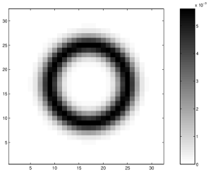
Figure 1: Response for a single Compton scatter angle for a unit source located at pixel (16,16). This response is normalized to unit integral. Units are counts.

To illustrate some aspects of the discussion above, we will show some results from an idealized scenario, as well as a more realistic simulation. As in K94, we employ a typical Compton telescope response for a single Compton scatter angle. The idealized PSF is computed over a $32\times 32$ pixel grid, and shown in Figure 1. For simplicity, we don’t worry about finite size or edge effects, and simply assume the PSF is normalized to unity, and wrap it around the boundaries as appropriate. The response $R$ is computed from all possible translates of this PSF.

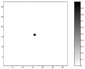
Figure 2: Test case 1, unit source at pixel (16,16). The corresponding “data” is noise-free, and simply given by the PSF in Figure 1.

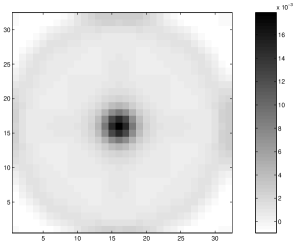
Figure 3: Estimated inverse for test case 1 via eqn. 15. Note that even though the data is noise-free, we have substantially underresolved the source.

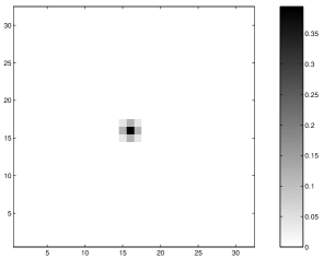
Figure 4: Estimate for test case 1, using 100 steps of the iteration of eqn. 13.

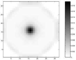
Figure 5: Estimate for test case 1, using 100 steps of the iteration of Paper I, given by eqn. 12.

Our first example is a unit source located at $(16,16)$, shown in Figure 2. The “dataset” is simply the corresponding PSF, with no background or noise added. Solution via eqn. 5 gives, not surprisingly, the exact answer, i.e. Figure 2. The regularized solution of eqn. 15 is shown in Figure 3, while the answer after 100 iterations of eqs. 13 and 12 are shown in Figures 4 and 5 respectively. Note that Figure 3 is quite spread compared to Figure 2, despite the fact that there is no noise or background in the “data”. This is an admittedly extreme example, but a properly regularized technique would allow one to take the statistics into account by varying the degree of regularization. The cancellation of the singular values in eqn. 15 implies that the $b_{i}$ corresponding to small singular values get larger weight in the solution. Since these $b_{i}$ typically correspond to large-scale or smooth functions, oversmoothing is not a surprising effect. Comparison of Figures 4 and 5 also demonstrate this limitation, since the results from eqn. 12 are inherently limited to be no better than the solution of eqn. 15 in terms of resolving power.

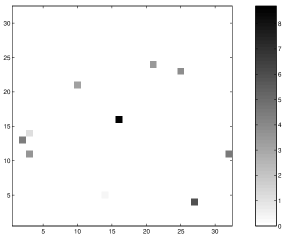
Figure 6: Test case 2, with multiple point sources of various strengths.

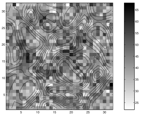
Figure 7: Data for test case 2, with a uniform background added to give an integrates source-to-background ratio of 10%, and Poisson noise. The overplotted contours show the noise-free data. Units are counts.

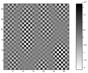
Figure 8: Direct least-squares estimate for test case 2. The large positive/negative fluctuations are the result of noise amplification from small singular values.

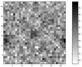
Figure 9: Estimate for test case 2 from eqn. 15. Note that the solution in much more stable compared with Figure 8, though noise roughly of the same magnitude as in the data is present, as expected from the orthonormality of $A$ and $B$.

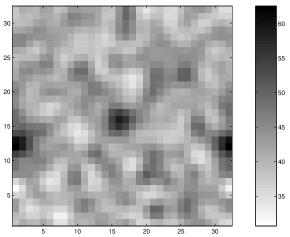
Figure 10: Estimate for test case 2 after 100 steps of the iteration of Paper I (eqn. 12). Note some regularization compared to Figure 9, due solely to stopping the iteration before convergence. Examination of Figure 9 indicates that non-negativity does not play a role, since due to the background level the stable fixed point solution is everywhere positive.

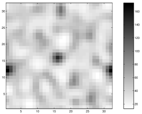
Figure 11: Estimate for test case 2 from the 100th iteration of eqn. 13.

Figure 12: Estimate for test case 2 after 100 steps of EMML (eqn. 21).

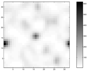
Figure 13: Estimate for test case 2 after 100 steps of yet another iteration, where we replace the $\Lambda$ term in the denominator of eqn. 12 with $\Lambda^{3}$.

The second example uses several point sources of varying intensity, shown in Figure 6. We generate data by convolution with the PSF and add a constant background such that the integrated source-to-background ratio is 10% (which would be extremely good for existing Compton telescopes, but useful for purposes of demonstration). Poisson random numbers are then generated for these expected count levels, resulting in the simulated data shown in Figure 7. For these simple examples, we make no attempt to fit or otherwise subtract the background, so the estimates will include a uniform background level as well. The least-squares solution is shown in Figure 8, and exhibits precisely the large oscillations we wish to suppress with regularization. The regularized direct solution of eqn. 15 is given in Figure 9; as we expect, the large oscillations are damped, since the small singular values have no effect, but plenty of noise is still evident. If we compare to Figure 10, computed via 100 iterations of of eqn. 12, we see better noise suppression. However, the result of 100 iterations of eqn. 13 in Figure 11 is certainly qualitatively better in terms of noise suppression and source resolution. The result from 100 steps of the EMML iteration of eqn. 21 is shown in Figure 12, and appears comparable with Figure 11. Just for fun, we also computed a result where we replaced the $\Lambda$ term in eqn. 12 with $\Lambda^{3}$ (there is a $\Lambda^{2}$ term implicit in eqn. 13). Shown in Figure 13, this map seems qualitatively better yet. Quantitatively, of course, only eqn. 13 will give correct photometry, since it corresponds to the case where we use the proper generalized inverse.

7 Final comments

I have shown above that the deconvolution method of Kebede (1994) appears to be erroneously derived. Kebede’s final expression (eqn. 12), however, does provide a regularized estimate of the inverse, where the regularization is caused by the exact cancellation of the singular values. It is left to the reader to decide if this is a positive characteristic of Kebede’s published algorithm, though the above discussion and examples would seem to indicate that it does not perform particularly well, even when compared with similar simple approaches. I have showed how to explicitly include statistical information, but also that much of this is lost due to the cancellation of the singular values.

I close with one final comment on the efficiency of the method. K94 claims that “…it takes very little computing time to run a program written based on this iterative method regardless of the size of the problem.” However, this is clearly not true. The computational complexity of SVD scales very badly with the problem size, going like the $aMN^{2}+bN^{3}$ for an $M\times N$ matrix ([Golub & Van Loan 1989]). For square image and data with $J\times J$ pixels, this would be $O(J^{6})$, which is terrible. Whether one uses eqn. 12 or eqn. 15, the SVD must be calculated explicitly, which would impose a heavy computational burden for all but very small images.

References

- [Campbell & Meyer 1979] Campbell, S. L. & Meyer, C. D. 1979, Generalized inverses of linear transformations (Copp Clark Pitman:Toronto).
- [Dixon et al.1996] Dixon, D. D. et al.1996, ApJ, 457, 789.
- [Ekstrom & Rhodes 1974] Eckstrom, M. P. & Rhodes, R. L. 1974, J. Comp. Phys., 14, 319.
- [Golub & Van Loan 1989] Golub, G. H. & Van Loan, C. F. 1989, Matrix Computations, 2nd ed. (Johns-Hopkins University Press:Baltimore).
- [Groetsch 1984] Groetsch, C. W. 1984, The Theory of Tikhonov Regularization for Fredholm Equations of the First Kind (Pitman:Boston).
- [Hebert, Leahy, & Singh 1990] Hebert, T., Leahy, R., & Singh, M. 1990, JOSA, 7, 1305.
- [Lucy 1974] Lucy, L.B. 1974, AJ, 79, 745.
- [Kebede 1994] Kebede, L. W. 1994, ApJ, 423, 878.
- [Knödlseder 1997] Knödlseder, J. 1997, Ph.D. Thesis, L’Universite Paul Sabatier.
- [Paige & Saunders 1982] Paige, C. C. & Saunders, M. A. 1982, ACM Trans. Math Software, 8, 43.
- [Richardson 1972] Richardson, W.H. 1972, JOSA, 62, 55.
- [Schönfelder et al.1993] Schönfelder et al.1993, ApJS, 86, 657.
- [van der Sluis & van der Vorst 1990] van der Sluis, A. & van der Vorst, H. A. 1990, Lin. Alg. Appl., 130, 257.
- [Wheaton et al.1995] Wheaton, Wm. A. et al.1995, ApJ, 438, 322.