The Sagittarius Dwarf Galaxy Survey (SDGS) I: CMDs, Reddening and Population Gradients. First evidences of a very metal poor population.

Abstract

We present first results of a large photometric survey devoted to study the star formation history of the Sagittarius dwarf spheroidal galaxy (Sgr dSph).

Three wide strips (size $\simeq 9\times 35~{}arcmin^{2}$) located at $\sim$($l^{o};b^{o}$)=(6.5;-16), (6;-14), (5;-12) have been observed. Each strip is roughly EW oriented, nearly along the major axis of the galaxy.

A control field (size $\simeq 9\times 24~{}arcmin^{2}$), located outside the body of Sgr dSph [$\sim$($l^{o};b^{o}$)=(354;-14)] has also been observed for statistic decontamination purposes.

Accurate and well calibrated V,I photometry down to V$\sim 22$ have been obtained for $\sim 90000$ stars toward the Sgr dSph and $\sim 8000$ stars in the control field.

This is the largest photometric sample (covering the widest spatial extension) ever observed in the Sgr dSph up to now.

The main new results presented in this paper are: (1) the possible discovery of a strong asymmetry in the distribution of stars along the major axis, since the north-western arm of the Sgr galaxy (i.e. the region nearer to the Galactic Bulge) apparently shows a significant deficiency of Sgr stars and (2) the first direct detection of a very metal poor (and presumably old) population in the Sgr stellar content. Hints for a metallicity gradient toward the densest region of the galaxy are also reported.

1 Introduction

The Sgr dSph is the most prominent member of the family of dwarf spheroidals orbiting the Milky Way (MW) both in luminosity ($\sim 10^{7}L_{\odot}$) and extension on the sky (at least $22\times 8$ degrees). In addition, it is by far the galaxy nearest to the Sun [see Ibata et al. 1997 (IGWIS); Ibata, Gilmore & Irwin 1995 (IGI-II) and references therein].

Since its discovery by Ibata, Gilmore & Irwin (1994, hereafter IGI-I), it was realized that the accurate study of this stellar system could help to shed light on many hot topics of modern astrophysics, as for example the formation and evolution of low surface brightness galaxies, the nature and extent of the dark matter halo in dwarf galaxies and the phenomenon of accretion of galactic sub-units by a main disc galaxy [see IGWIS and Montegriffo et al. (1998, hereafter MoAL) for discussions and references]. A huge observational and theoretical effort has been addressed to the study of Sgr dSph in the past three years and the research is still flourishing. We summarize here only the main observational results, the reader interested to the theoretical simulations can find many useful references in IGWIS, Hernandez & Gilmore (1998), Zhao (1998), Ibata & Geraint (1998) and Johnston (1998).

¿From a dynamical point of view, an estimate of the orbital period of the galaxy has been obtained ($\sim 1~{}Gyr$) and strong cases have been made for the presence of a highly concentrated and massive dark matter halo (IGWIS, Hernandez & Gilmore 1998). The projected structure has been mapped over a $\sim 15\times 15~{}deg$ field by IGWIS, but many authors claimed the detection of Sgr stars far away from the edges of the IGWIS isodensity map (Alard 1995, Siegel et al. 1997). A huge project aimed to map the spatial structure of Sgr using RR Lyrae stars is currently carried on by the OGLE collaboration (Lepri et al. 1997).

H I observations (Koribalski, Johnston & Otrupcek 1998) put a strong upper limit on the gas content of the galaxy ($\sim 10^{4}M_{\odot}$, i.e. less than $10^{-3}$ of the total mass) confirming the classification of Sgr as a classical dwarf spheroidal galaxy (gas is generally missing in such galaxies, see Koribalski, Johnston & Otrupcek 1998, and references therein).

Studies of the stellar content of Sgr has revealed the presence of carbon stars (Whitelock, Irwin & Catchpole 1996, hereafter WIC), planetary nebulae (Zjilstra & Walsh 1996; Walsh et al. 1997) and RR Lyrae stars (Mateo et al. 1995a, 1995b; Alard 1996; Alcock et al. 1996). Color-Magnitude Diagrams (CMD) of Sgr stars have been obtained by Mateo et al. (1995a; MUSKKK), Sarajedini & Layden (1995; SL95) and Marconi et al. (1997; MAL) while the properties of the globular cluster system of the Sgr galaxy have been reviewed and discussed by MoAL. Useful constraints about Sgr age and metallicity have also been found by Fahlman et al. (1996), Mateo et al. (1995b; hereafter MKSKKU) and Mateo et al. (1996). The resulting scenario can be summarized as follows:

• The dominant stellar population (hereafter Pop A) of the Sgr dSph is younger (by $\sim 4-5~{}Gyr$) than classical old galactic globulars (MUSKKK, MAL, Fahlman et al. 1996). MAL found that the main loci of Pop A CMD nearly coincide with those of the young and metal rich globular cluster Ter 7 (see Fusi Pecci et al 1995, and references therein), which belong to the Sgr globular cluster system (see MoAL). Average metallicity estimates ranges from $[Fe/H]=-1.1$ (MUSKKK) to $[Fe/H]\simeq-0.6$ (SL95). All authors, however, agree on the presence of a metallicity spread, and the coexistence of at least two distinct components into the main population has been suggested by SL95. Preliminary results from high resolution spectroscopy on a small sample of Sgr stars (Smecker-Hane , Mc William & Ibata 1998) point toward an even larger spread in metal abundance, finding stars with metallicity from $[Fe/H]=-1.5$ to $[Fe/H]=+0.11$.

• The simultaneous presence of a clear sequence of blue stars (Blue Plume, see below) and Carbon Stars have been interpreted as an evidence for the presence of a sparse population of stars significantly younger than Pop A (MUSKKK; WIC; Layden & Sarajedini 1997, hereafter LS97). Let us call this component Pop B, for brevity. The estimates of the absolute age of Pop B range from 4 Gyr (MUSKKK) to 1 Gyr (Ng 1997).

• There are at least two (of the four) globular clusters associated with Sgr that are very metal poor ($[Fe/H]\sim-2$) and significantly older than Pop A, i.e. M54 (MAL, LS97) and Terzan 8 (MoAL). This fact, coupled with the presence of RR Lyrae stars, suggest the existence of an old and metal poor population in the galaxy. However a direct identification of such a component is still missing.

It is evident that many important pieces of information are still uncertain or missing and we are still far from having a satisfactory scenario for the star formation and chemical enrichment history of Sgr. However, deriving clear-cut information from the CMDs of this galaxy is prevented by two fundamental factors:

1. [rm]

2. Sgr dSph is projected onto a region of the sky highly contaminated by stars belonging to the central bulge and disc of the Milky Way;

3. the intrinsically low surface brightness ($\mu_{V}(0)\sim 25.5~{}mag/arcsec^{2}$) coupled with the relatively small distance from the sun ($\sim 25~{}Kpc$) implies that it is necessary to observe wide regions of the galaxy to sample a significant number of member stars. The sampling of stars in the post-MS phase is particularly critical because of the short lifetimes, corresponding to low number densities (see Renzini & Fusi Pecci 1988).

This latter point is fundamental in order to perform a fruitful quantitative analysis of the Sgr stellar content. Assuming that Sgr be a Simple Stellar Population (Renzini & Fusi Pecci 1988) of age $\sim 10~{}Gyr$ and $\mu_{V}(0)\sim 25.5~{}mag/arcsec^{2}$, $(m-M)_{0}=17.01$ and $A_{V}=0.55$ (MUSKKK), and following the prescriptions of Renzini (1998) and Maraston (1998), the number of stars in each evolutionary phase sampled by a given field of view can be roughly estimated. Supposing, for instance, to image the densest region of Sgr with a field of view of $10\times 10~{}arcmin$ we expect to sample only $\sim 300-400$ stars from the base to the top of the Red Giant Branch (RGB) and $\sim 50$ stars in the whole Horizontal Branch (HB). A HST-WFPC field would sample only $\sim 15$ RGB stars and $\sim 2$ HB stars.

The former problem can be circumvented (at least partially) by careful statistical decontamination, using the CMD of stars representative of the contaminating population (see MUSKKK as an example). However the success of any statistical decontamination depends on how well are defined the sequences of the underlying population on the CMD. It is evident that both point (i) and (ii) can be successfully afforded only sampling wide regions of the galaxy.

In this paper we present a photometric survey of the Sgr dSph covering a total field of view of $954~{}arcmin^{2}$. We obtained accurate V and I photometry for 89858 stars (by far the largest CCD sample of Sgr stars to date), sampling three regions of the galaxy $\sim 2^{o}$ apart from each other and located nearly along the major axis ($l\sim 5^{o}$, see IGI-I, IGI-II and IGWIS).

Two out of the three sampled regions included the fields recently surveyed with HST (GO 6614, PI: K. Mighell) and for which very deep photometry (down to $\sim 4~{}mag$ below the MS-TO of Pop A) has been obtained (Mighell et al. 1997). Since the limiting magnitude of the SDGS is V$\sim 22$ (just below the Sgr Pop A Turn Off), the present study is the natural complement to the deep (but “small field”) photometry by Mighell et al. (1997).

Given the amount of collected data and the time needed to perform a complete and quantitative analysis, we decided to present the SDGS results in two papers. One considerable benefit of this approach is to provide the astronomical community with the largest photometric database of Sgr stars and many useful guidelines for future observations before the full completion of our analysis.

The present paper (Pap I) is devoted to the general description of the survey, and to set the basis for a detailed study of the Star Formation History of the Sgr dSph .

We discuss data reductions, photometric calibration and completeness of the samples (sect. 2). The CMD are shortly presented (sect. 3) and the differences in interstellar reddening between the different fields are estimated (sect. 4). Previous studies have shown that many useful things can be learned from Sgr CMDs before (and/or without) performing statistical decontamination of the whole diagrams (MUSKKK, SL95, MAL). We include here also many tests devised to study the Sgr stellar populations and their projected spatial distribution, either using the “raw” (foreground contaminated) CMDs (sect. 5 and sect. 6) or attempting to remove the contribution of foreground stars from star counts in small selected box on CMDs (see sect. 5.5). The derived results and suggestions will be used as a guideline and independent check for the forecoming analysis. A final summary is reported in sect. 7.

The companion paper (Bellazzini et al. 1998b; Pap II, in preparation) will be devoted to the detailed analysis of statistical decontaminated CMDs, specifically aimed to the study of the Star Formation History in Sgr.

2 Description of the SDGS

The main purpose of the SDGS was to sample a statistically significant number of evolved stars in the Sgr dSph . A wide area of sky was covered using a “snapshot survey technique”, i.e. taking relatively short (V,I) exposures (long enough to reach the TO level) in many different fields using a camera with a wide field of view. Two nights (27 - 28, June 1997) at the ESO 3.5 m New Technology Telescope (NTT) were allocated to this project .

We used the EMMI camera with the RILD setup (Zjilstra et al. 1996). This instrument provides an optically corrected and unvignetted field of $9.15\times 8.6~{}arcmin$. The detector was a Tek CCD ($2048\times 2048$ pxs, pixel size $24\mu m$) with a read-out noise of $3.5e^{-}$ rms, a dark current of $3e^{-}/hr$ and a gain factor of 1.34 $e^{-}/ADU$. The image scale is $0.27~{}arcsec/px$. The filters used are ESO 606 (V) and ESO 610 (I). In the best cases we acquired a long (300 s) and a short (60 s) exposure in each filter.

We observed three strips (nearly E-W oriented, i.e. approximately along the Sgr major axis) each composed by five partially overlapping fields. An overlapping area of nearly $1.5~{}arcmin$ has been secured between each couple of adjacent fields in order to obtain a robust relative photometric calibration in each strip.

As already mentioned , the location of two strips has been chosen to include the fields covered by deep HST observations:

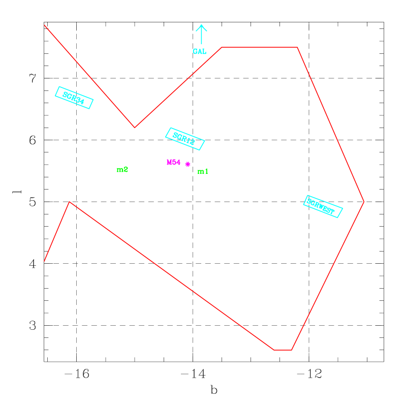
Figure 1: A map in galactic coordinates representing the position of the observed fields within the Sgr galaxy. The heavy line roughly reports the limit of the outer isodensity contour of the IGWIS map (their fig. 1). The position of SGR34, SGR12 and SGRWEST strips is reported; the arrow at the top of the panel indicates the direction toward the control GAL field. The position of the M54 globular cluster is indicated by an asterisk and the location of the two fields observed by MAL is indicated by the labels m1 and m2. The field observed by MUSKKK is included in SGR34, the Sgr field observed by SL95 is included in SGR12. The small fields observed with HST by Mighell et al. (1997) are included in SGR34 and SGR12.

A first strip, located near the center of density of Sgr (IGWIS) and extending from ($l=5.8^{o};b=-13.9^{o}$) to ($l=6.0^{o};b=-14.4^{o}$), includes the HST fields labeled Sgr 1 ($\alpha_{2000}=18~{}h~{}55~{}m~{};~{}\delta_{2000}=-30^{o}~{}16^{\prime}$; also observed by SL95) and Sgr 2 ($\alpha_{2000}=18~{}h~{}55~{}m~{};~{}\delta_{2000}=-30^{o}~{}14^{\prime}$); hereafter we will call it SGR12 strip.

A second strip, located $\sim 2^{o}$ eastward of SGR12 and extending from ($l=6.6^{o};b=-16.2^{o}$) to ($l=6.5^{o};b=-15.8^{o}$), include the HST fields labeled Sgr 3 ($\alpha_{2000}=19~{}h~{}06~{}m~{};~{}\delta_{2000}=-30^{o}~{}25^{\prime}$) and Sgr4 ($\alpha_{2000}=19~{}h~{}06~{}m~{};~{}\delta_{2000}=-30^{o}~{}23^{\prime}$; both fields were also observed by MUSKKK); hereafter we will call it SGR34 strip.

A third strip was observed in a still “unexplored” region of Sgr, westward of SGR12, from ($l=4.9^{o};b=-12.1^{o}$) to ($l=4.7^{o};b=-11.5^{o}$); hereafter we refer to this strip as SGRWEST, since the sampled region can be considered as the north-western arm of the Sgr galaxy. This is the field observed at the lowest galactic latitude: it was selected to study the Sgr population in a region where the interaction with the Galaxy should be stronger (according to IGWIS, this is the region of the Sgr dSph that is leading the galaxy along its orbit, and so will be the first one to “collide” with the Galaxy during the present perigalactic passage). It is important to note that SGR34 and SGRWEST fields are nearly symmetrically located with respect to the center of density of the Sgr dSph (SGR12), along the major axis: SGRWEST is $2^{o}$ from the center in the direction of the Galactic Bulge, while SGR34 is $1.6^{o}$ in the opposite direction.

In addition we observed a control field in a region devoid of Sgr stars and dominated by foreground Galactic field stars. This field has been observed with the same “strip technique” described above, but only three - partially overlapping - EMMI fields have been observed in this case. The Galactic field strip include the control field labeled SGR-MWG1 and SGR-MWG2 in the HST-GO 6614 proposal and also observed by MUSKKK, around ($\alpha_{2000}=18~{}h33~{}m~{};~{}\delta_{2000}=-40^{o}~{}56^{\prime}$); we will call this strip the GAL field.

Bad weather conditions and some technical problem occurred during the allocated nights prevented us from observing two additional strips (located between SGR12 and SGR34) which were originally planned to complete the SDGS.

The location (in Galactic Coordinates) and approximate dimensions of the fields covered by the SDGS are presented in fig. 1. The heavy line roughly represent the most external isodensity line of the IGWIS map (their fig. 1). The position of the fields observed by MAL is also reported. The arrow indicates the direction toward the GAL field which lies outside the limits of the figure but is located at the same Galactic latitude of SGR12.

2.1 Observations

The log of the observations is presented in Table 1. A grand total of 58 frames has been obtained.

Each field within a given strip has been named A, B, C, etc., in sequence, assigning label A to the frame used as reference frame for the relative calibration within the strip (see sec. 2.2). The columns of Table 1 reports, in order, the name of the observed field, galactic longitude ($l^{o}$) and latitude ($b^{o}$) of the center of the field, the adopted filter, the exposure times and the seeing conditions (FWHM of the Point Spread Function).

Table 1: Observations report.

Field	$l^{o}$	$b^{o}$	Filter	Exp.	Seeing
Name				time	(FWHM)
SGR12 A	5.99	-14.36	V	300, 60 s	$1.92^{{}^{\prime\prime}}$
SGR12 A	5.99	-14.36	I	300, 60 s	$1.71^{{}^{\prime\prime}}$
SGR12 B	5.95	-14.27	V	300, 60 s	$1.90^{{}^{\prime\prime}}$
SGR12 B	5.95	-14.27	I	300, 60 s	$1.57^{{}^{\prime\prime}}$
SGR12 C	5.91	-14.17	V	300, 60 s	$1.87^{{}^{\prime\prime}}$
SGR12 C	5.91	-14.17	I	300, 60 s	$1.51^{{}^{\prime\prime}}$
SGR12 D	5.87	-14.08	V	300, 60 s	$2.23^{{}^{\prime\prime}}$
SGR12 D	5.87	-14.08	I	300, 60 s	$1.40^{{}^{\prime\prime}}$
SGR12 E	5.83	-13.99	V	300, 60 s	$2.81^{{}^{\prime\prime}}$
SGR12 E	5.83	-13.99	I	300, 60 s	$1.46^{{}^{\prime\prime}}$
SGR34 A	6.66	-16.26	V	300 s	$1.24^{{}^{\prime\prime}}$
SGR34 A	6.66	-16.26	I	300 s	$1.34^{{}^{\prime\prime}}$
SGR34 B	6.62	-16.17	V	300 s	$1.28^{{}^{\prime\prime}}$
SGR34 B	6.62	-16.17	I	300 s	$1.22^{{}^{\prime\prime}}$
SGR34 C	6.58	-16.07	V	300, 60 s	$1.59^{{}^{\prime\prime}}$
SGR34 C	6.58	-16.07	I	300, 60 s	$1.34^{{}^{\prime\prime}}$
SGR34 D	6.54	-15.98	V	300, 60 s	$1.43^{{}^{\prime\prime}}$
SGR34 D	6.54	-15.98	I	300, 60 s	$1.46^{{}^{\prime\prime}}$
SGR34 E	6.50	-15.89	V	300, 60 s	$1.34^{{}^{\prime\prime}}$
SGR34 E	6.50	-15.89	I	300, 60 s	$1.41^{{}^{\prime\prime}}$
SGRWEST A	4.92	-12.01	V	300 s	$1.12^{{}^{\prime\prime}}$
SGRWEST A	4.92	-12.01	I	300 s	$1.22^{{}^{\prime\prime}}$
SGRWEST B	4.87	-11.91	V	300 s	$1.20^{{}^{\prime\prime}}$
SGRWEST B	4.87	-11.91	I	300 s	$1.40^{{}^{\prime\prime}}$
SGRWEST C	4.82	-11.80	V	300 s	$1.20^{{}^{\prime\prime}}$
SGRWEST C	4.82	-11.80	I	300 s	$1.16^{{}^{\prime\prime}}$
SGRWEST D	4.78	-11.72	V	300 s	$1.18^{{}^{\prime\prime}}$
SGRWEST D	4.78	-11.72	I	300 s	$1.37^{{}^{\prime\prime}}$
SGRWEST E	4.72	-11.59	V	300 s	$1.16^{{}^{\prime\prime}}$
SGRWEST E	4.72	-11.59	I	300 s	$1.12^{{}^{\prime\prime}}$
GAL A	353.88	-14.25	V	300, 60 s	$1.43^{{}^{\prime\prime}}$
GAL A	353.88	-14.25	I	300, 60 s	$2.12^{{}^{\prime\prime}}$
GAL B	353.77	-14.30	V	300, 60 s	$1.46^{{}^{\prime\prime}}$
GAL B	353.77	-14.30	I	300, 60 s	$1.95^{{}^{\prime\prime}}$
GAL C	353.67	-14.35	V	300, 60 s	$1.50^{{}^{\prime\prime}}$
GAL C	353.67	-14.35	I	300, 60 s	$1.38^{{}^{\prime\prime}}$

As shown in Tab. 1, the seeing conditions were never particularly good but were remarkably stable when the SGR34 and SGRWEST fields were observed.

On the contrary, significant seeing variations has been encountered during the acquisition of the SGR12 frames. The net result was a brighter limiting magnitude for SGR12 frames with respect to SGR34 and SGRWEST, and a bad quality Color Magnitude Diagram below $V\sim 19$ for the fields SGR12 D and E (only stars with $V\leq 18.5$ from these two fields will be included in the final CMD of the SGR12 strip, see below).

GAL frames were obtained during the moon rising phase (nearly at the end of the night), and show a high average sky level, resulting in a brighter limiting magnitude with respect to SGR34 and SGRWEST.

Short exposure frames are missing for SGR34 A and B fields and for the whole SGRWEST strip. This is not a serious problem for our purposes, since the RGB tip of the Sgr Pop A is located at $V\sim 16$ while the saturation level of the SDGS long exposures occurs at $V\sim 15.5$, even in the best seeing conditions. Thus we are confident that even the images of the brightest Pop A giants are not significantly saturated; however their position in the CMD may be affected by larger uncertainties (with respect to the cases when also short exposures were secured) since they could have been observed in the non-linear regime of the CCD response.

2.2 Data reduction

All the frames were trimmed, bias subtracted and flat-fielded, with high S/N flat field frames secured at the beginning and the end of the nights. The pre-reduction procedures were done using the MIDAS package.

The photometric reductions were carried out using the ROMAFOT package (Buonanno et al. 1983, and references therein) mounted on a Digital-Alpha station of the Bologna Observatory. A standard two-dimensional PSF fitting procedure was performed on the pre-reduced frames. In order to determine the PSF and to find and fit stars in each frame, we adopted the standard procedure as described, for example, by Ferraro et al. (1990). The PSF parameters were allowed to vary as a function of position in the frame, to account for slight differences in the images shape across the wide EMMI field of view.

The program stars were detected automatically adopting a threshold-criterion ($\sim 5\sigma$) above the local background level, for the deep exposures, and ($\sim 6\sigma$) for the short ones. The searching procedure was performed on the V frames, and the list of identified sources were used as input for the PSF fitting in the corresponding I frames.

The instrumental magnitudes of each frame in a given strip were referred to the instrumental magnitudes of the frame assumed as a reference (i.e. A fields). Stars in common in the overlapping region (typically $\sim 1500$ for each couple of adjacent fields) were used to determine the transformations between instrumental magnitudes of a given frame and the reference frame. The transformations were always well defined and never larger than few hundredths of magnitude. The uncertainty in the relative frame-to-frame calibration within a strip is $\sim 0.01~{}mag$ (conservative estimate).

Figure 2: Internal photometric errors in each observed strip. The magnitude differences for stars in common between two adjacent fields is plotted versus the V mean magnitude. In all cases the photometric uncertainty is $<0.05mag$ (dashed line) for stars brighter than $V=19$.

2.3 Photometric errors

The best empirical estimate of the internal accuracy of a photometric data set is usually derived from the rms of repeated measures of selected stars. We used stars in the overlapping regions: the magnitude differences for these stars as a function of V magnitude are plotted in fig. 2. We assume the standard deviation around zero (computed in bins 1 mag wide) of the magnitude differences as a conservative estimate of the average photometric uncertainty in the corresponding magnitude bin. For each considered strip, the trend of the photometric error with V magnitude was optimally fitted with a polynomial, and so it has been possible to associate a typical photometric error to each star, as a function of its V magnitude. As can be seen from fig. 2, the internal accuracy is better than 0.05 mag for the large majority of the measured stars.

2.4 Absolute calibration

Several CCD standard fields (Landolt 1993) were acquired during both the nights in order to provide an accurate absolute calibration. A total of 23 standard stars, covering a wide range of colors, were used to link the instrumental aperture magnitudes to the standard Johnson system.

The reduction of standard star observations and the determination of aperture correction for the science frames has been performed with a standard technique, using the appropriate task of ROMAFOT devoted to aperture photometry.

In fig. 3, the differences between standard (V,I) and instrumental (v,i) aperture magnitudes vs. instrumental color index are reported. Since the slope is negligible with respect to the dispersion around the mean we decided to exclude color terms in the adopted calibration equations. The final adopted equations are the following:

$$V=v+25.21\pm 0.02$$

$$I=i+24.61\pm 0.02$$

where the error is a conservative estimate of the uncertainty in the absolute calibration.

A set of most isolated, unsaturated stars in the reference frames were then used to link the “aperture” magnitudes to the PSF-fitting instrumental magnitudes. The “fit-to-aperture” corrections applied introduces an extra zero-point uncertainty of $\sim 0.02$ mag in each color and has to be regarded as the major source of uncertainty in the absolute calibration of the stars in each strip of SDGS.

Figure 3: Calibration curves as a function of instrumental (v-i) color for the observed Landolt stars. Different symbols refer to stars observed during different nights: June, 27 (open circles) and June, 28 (filled circles), respectively.

The calibrated data are available via anonymous FTP at hopi.bo.astro.it in the directory /home/ftp/pub/michele/SDGS-I.

2.5 Completeness of the samples

The crowding conditions in the observed fields are not critical ($0.03~{}stars/arcsec^{2}$ in the worst case) and are very homogeneous in general. This suggests that the completeness level should be not very different from field to field, at least within a given strip. Some preliminary artificial star test confirmed this expectation. Thus we decided to perform extensive artificial star experiments in one field for each strip, assumed to be representative of the whole strip sample, namely SGR12 B, SGR34 C, SGRWEST B and GAL C.

A total of nearly 4000 artificial test stars were added to each selected field, never more than 100 each time, in order to leave unaltered the crowding conditions. The test stars were chosen with a color representative of the mean color of the sampled population. A square sub-image containing the selected star were extracted from the original frame and randomly added to the frame. The entire reduction procedure has been repeated in the same way on the synthetically enriched images. The ratio between the number of simulated stars recovered with a magnitude within $\pm 0.1~{}mag$ from the original test star, and the total number of artificial images added was taken as the completeness factor ($C_{f}$) in the corresponding magnitude bin. The typical uncertainties on the completeness factors is $\leq 5\%$.

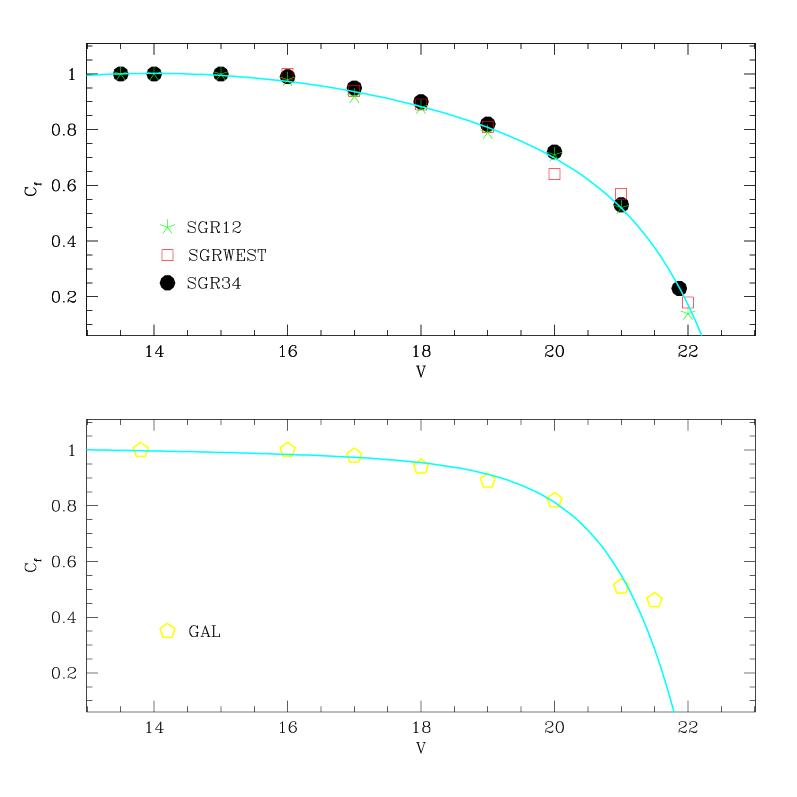
Figure 4: Completeness factor as a function of V magnitude for the SGR12 B, SGR34 C and SGRWEST B fields (upper panel) and for the GAL C field. The reported lines are best fit curves to the data. The resulting completeness functions is adopted as representative of the whole sample in a strip: the curve in the upper panel is used for SGR12, SGR34 and SGRWEST (since the differences among the measured completeness factors are negligible); the curve in the lower panel is used for the GAL strip. The uncertainty on each completeness factor is $\leq 5\%$.

The results of the completeness experiments for SGR12 B, SGR34 C and SGRWEST B are reported in the upper panel of fig. 4. It is evident that the completeness factors for this three fields are the same within the errors in the common range of magnitude ($16<V<21$). This is not unexpected since the crowding conditions are nearly similar and in any case very far from the critical conditions found, for instance, in the central region of globular cluster images. Furthermore the (x,y) distribution of stars is very homogeneous so there is no expected variation of the completeness with position. This results provide a robust support to use the derived completeness as representative of the whole considered strips, since it has been demonstrated that the observed field to field variations have a minimal impact on the overall completeness.

We decided to adopt a unique completeness function for the three quoted strip, which is plotted as a solid curve in figure 4 (upper panel). Note that $C_{f}$ falls below 0.5 only at $V\simeq 21$ and is $>0.8$ for $V\leq 19$.

A distinct completeness function is adopted for GAL (fig. 4, lower panel), since little but significant differences are present, with respect to the Sgr strips. Higher values of $C_{f}$ are found in the range ($18<V<20$), probably because of the significantly lower stellar density (i.e. better crowding conditions).

If not otherwise stated, any star count will be hereafter corrected for completeness using the completeness functions presented in fig. 4, in the range from the brighter unsaturated stars to the level where $C_{f}$ fall below 0.5.

A useful by-product of the artificial stars experiments, is an independent check of the ability of the photometry code to reproduce the same result in repeated measures of the same stars. The standard deviation of the difference between the original magnitude of a given star and the derived magnitude of the recovered copies artificially distributed in the frame was found to be always significantly less than the adopted total photometric error described in sect. 2.3.

3 Color Magnitude Diagrams

3.1 Homogeneity of the samples

Following the procedure described in sec. 2.2, a CMD for each EMMI field has been obtained. The single-field CMDs in each strip have been compared in order to check for possible systematic differences in reddening (see below) and stellar content within each strip. Moreover, specific population ratio tests in selected region of the CMDs were performed to obtain quantitative intercomparisons. No significant difference in the distribution of stars in the CMD emerged from these tests, the stellar content within each strip turned out to be very homogeneous. For this reason we decided to merge the sample of each field of any given strip in one single database for each strip. For the stars lying in the overlapping regions, the average magnitude between the two available measures has been adopted.

Visual inspection of single-field CMDs also suggested that the possible impact of differential reddening within each strip must be negligible.

A further check was made possible by the availability of the new DIRBE/IRAS All-Sky Reddening Maps (ASRM; Schlegel, Finkbeiner & Davis 1997, 1998) which allow reddening estimates with a spatial resolution of $\sim 6~{}arcmin$ and a typical accuracy of $\sim 16\%$, so superseding the widely used maps by Burstein & Heiles (1982).

We calculated from ASRM (see Stanek 1998, for details of the procedure) the E(V-I) in the center position of each EMMI single field interpolating from four adjacent resolution elements of the map. The derived reddening differences among fields in each strip are always small, the maximum difference being less than 0.02 mag. The standard deviation about the mean E(V-I) value of single fields [$\sigma_{E(V-I)}]$ amounts to 0.01 mag for SGR34 and SGRWEST, to 0.015 for GAL and to 0.005 for SGR12 [see also table 2, below; we adopted all over the paper the following relations: $E(V-I)=1.6\times E(B-V)$ and $A_{V}=1.93\times E(V-I)$; from Rieke & Lebovsky 1985, hereafter RL]. With this further support, we conclude that any possible differential reddening between single fields is of the same order of the uncertainty of the relative calibration or less, and so negligible for the present purposes.

In conclusion we can state that, at the present level of accuracy, the stars in each strip can be considered as an homogeneous sample from any point of view.

Hereafter, any distinction between sub-fields within a strip is therefore useless and we will refer to the whole strip samples with the labels SRG12, SGR34, SGRWEST and GAL Fields (capital letter). We will refer to the sample of stars from the SGR12 A, B and C fields alone with the label SGR12R (Restricted).

3.2 The global CMDs

In figures 5, 6, 7 and 8 the total CMDs of the three Sgr strips and of the control field are displayed. In fig. 5, only the stars belonging to SGR12 A, B and C fields are reported since, as already mentioned, the faint part of SGR12 D and E CMDs have poor photometric quality.

Figure 5: Color Magnitude diagram for all the stars measured in the A, B, C fields of the SGR12 strip (16992 stars).

Here we make only few comments on the CMDs, mainly comparing the Sgr CMDs to the control field one. Deeper insights will be added in sec. 5 after the discussion of reddening.

The main general features of the CMDs are the following:

1. apart from the different photometric quality, SGR34 (fig. 6) and SGR12 (fig. 5) diagrams are very similar and show all the characteristics of the typical Sgr CMDs (MUSKKK, SL95, MAL). The bulge+disc contaminating population (compare with the control filed CMD in fig. 8) produce a pronounced blue sequence at $V-I\sim 0.8$, that is nearly vertical from $V\sim 15$ to $V\sim 20$ where it become a large band sloped toward redder colors. A sparser feature runs near parallel to the vertical part of this sequence, at slightly redder color ($V-I\sim 0.9~{}-~{}0.1$), and can be identified with the giant branch of the bulge population.

2. The Sgr population is clearly evident as a globular cluster-like sequence with a Main Sequence Turn Off (MSTO) around ($V\sim 21.5;V-I\sim 0.7$), a well defined (at least in the SGR34 CMD) Sub Giant Branch (SGB),a wide Red Giant Branch (RGB) extending to ($V\sim 16;V-I\sim 2.5$) and a clear red Horizontal Branch (HB) at ($V\sim 18-18.3;V-I\sim 1$). The SGR12 HB appears more clumped to the red with respect of that of SGR34. In the SGR34 and SGR12 fields this globular cluster-like population is clearly the dominant feature of the CMDs (Pop A).

   The blue plume discussed by MUSKKK, SL95, Ng (1997), LS97, and identified with a young component (Pop B, see above) is clearly present at ($V\sim 20;V-I\sim 0.4$)

   Figure 6: Color Magnitude diagram for all the stars measured in the SGR34 strip (22603 stars).

3. The SGRWEST CMD appears dominated by the contaminating population, in particular the bulge MS. The MSTO of the bulge seems to emerge from the vertical blue sequence at ($V\sim 18-19;V-I\sim 0.8$). However the signatures of the Sgr population are still present, in particular the sparse RGB plume and the red HB. The Sgr TO and SGB are not well defined but their presence is strongly suggested by a clear excess of stars in the region around $V\sim 21.5$ and $V-I\sim 0.6-1.0$, with respect to the GAL CMD.

Figure 7: Color Magnitude diagram for all the stars measured in the SGRWEST strip (41462 stars).

The comparison of the CMDs in fig. 5, 6, 7 with the corresponding ones derived by other authors (MUSKKK for SGR34 and GAL; SL95 for SGR12; MAL) shows, in general, an excellent agreement. The positions of the main loci are compatible within the photometric errors and any possible disagreement in the absolute calibration can be considered negligible. The most robust comparison can be performed between SGR34 and the MUSKKK CMDs, since they are similar both in limiting magnitude level and in overall photometric quality. The agreement is very good. In Pap II we will take advantage of the deeper control field CMD obtained by MUSKKK at the same position of the GAL strip to properly decontaminate the TO region of our Sgr CMDs.

Figure 8: Color Magnitude diagram for all the stars measured in the control field, the GAL strip (8336 stars).

4 Reddening

Once stated the homogeneity of the samples within Fields we can turn to study the possible differences among the observed Fields. Before discussing the stellar content of the Fields it is advisable to check if the SGR12, SGR34, SGRWEST and GAL Fields are affected by different amount of interstellar extinction and reddening.

4.1 Differences between SDGS Fields

At present, there are two direct reddening estimates in Sgr regions sampled by SDGS, i.e. $E(V-I)=0.22\pm 0.04$ for SGR34 (MUSKKK) and $E(B-V)=0.13\pm 0.02$ for SGR12 (SL95), which corresponds to $E(V-I)=0.21\pm 0.03$ (RL). Thus the two measures agrees within the errors (but see SL95 for further discussions). No estimate exist for SGRWEST and GAL Fields, however MUSKKK implicitly assume that their Sgr field (a subsample of SGR34) and their control field (a subsample of GAL) have the same extinction.

The reddening measure by MUSKKK must be regarded as the most robust one, since it has been directly derived from the colors at minimum of 5 Sgr RR Lyrae stars. On the other hand SL95 used the SMR method (Sarajedini 1994, hereafter S94) devoted to simultaneously derive the metallicity and reddening from the observed RGB ridge line and Horizontal Branch luminosity ($V_{HB}$) of globular clusters (GC). In the present case the power of the method can be seriously weakened by the intrinsic wideness of the RGB, which on the contrary is usually very thin and well defined for GCs. Furthermore, Sgr population is almost certainly younger - and perhaps slightly more metal rich - than the Galactic globulars used to calibrate the SRM method. We plan to test the application of the SMR method to SDGS data only on decontaminated CMDs (Pap II).

Thus, we assume $E(V-I)=0.22\pm 0.04$ (MUSKKK) for SGR34 as an “absolute reddening zero-point” and try to determine eventual reddening difference between SGR34 and the others SDGS Fields by other means.

A first check has been performed using ASRM, as described in the previous section. It result (see tab. 2, below) that SGR12, SGR34 and SGRWEST have very similar reddening, and the absolute value is in excellent agreement with the direct estimates ($E(V-I)\sim 0.21~{}-~{}0.22$). A lower reddening is obtained for GAL ($E(V-I)\sim 0.14$). The agreement with the final adopted E(V-I) value for this Field (see below) is only marginal and this reddening estimate has to be regarded as the most uncertain of the whole set presented in table 2.

4.1.1 Matching sequences and HBs

A more reliable way to estimate the differential reddening between SGR34 and the others SDGS Fields can be achieved by the comparison of the mean position and blue edge in color of the vertical blue sequence of the contaminating population described in sec. 3 (hereafter VBS). This method has been already discussed and applied to Sgr by IGWIS. Here we slightly refine the procedure trying to simultaneously match the VBS distribution with a color shift $\Delta E(V-I)$ and the magnitude of the peak of the Sgr HB population with a corresponding magnitude shift $\Delta A_{V}=1.93\times\Delta E(V-I)$. Finding a $\Delta E(V-I)$ value that satisfactorily matches both the constraints provides also support to the statement that differential reddening is at the origin of the apparent shift eventually detected.

In figure 9, the results of the above procedure are reported. In left panels the color distribution of the blue sequence stars (selected to have $16.5<V<19.5$ and $0.6<V-I<0.95$) are displayed. Dashed line histogram refer to our “reddening reference Field”, i.e. SGR34, whilst solid line histograms refer to the SGR12 (upper panel), SGRWEST (middle panel) and GAL (lower panel) samples, respectively, after the appropriate $\Delta E(V-I)$ shift has been applied in order to match the compared distributions. The same symbols are adopted for right hand panels, presenting the histograms of the stars in the Sgr HB region (selected to have $17<V<19$ and $0.95<V-I<1.2$). The shifts have been computed in the following way, taking, as an example, the comparison between SGR34 and SGR12:

$$\Delta E(V-I)=E(V-I)_{SGR34}-E(V-I)_{SGR12}$$

$$\Delta A_{V}={A_{V}}_{SGR34}-{A_{V}}_{SGR12}$$

In the cases of SGR12 and SGRWEST the match is excellent, and it can be concluded that the tiny shifts observed are probably due to slight reddening differences. Though the reddening differences found (reported in the left panels of fig. 9) are, at most, only marginally significant, we decided to adopt them since they provide such a good match. This test also shows that any distance difference between different regions along the major axis due to the possible inclination of Sgr with respect to the line of sight is negligible, over the scale sampled by SDGS ($4^{o}$).

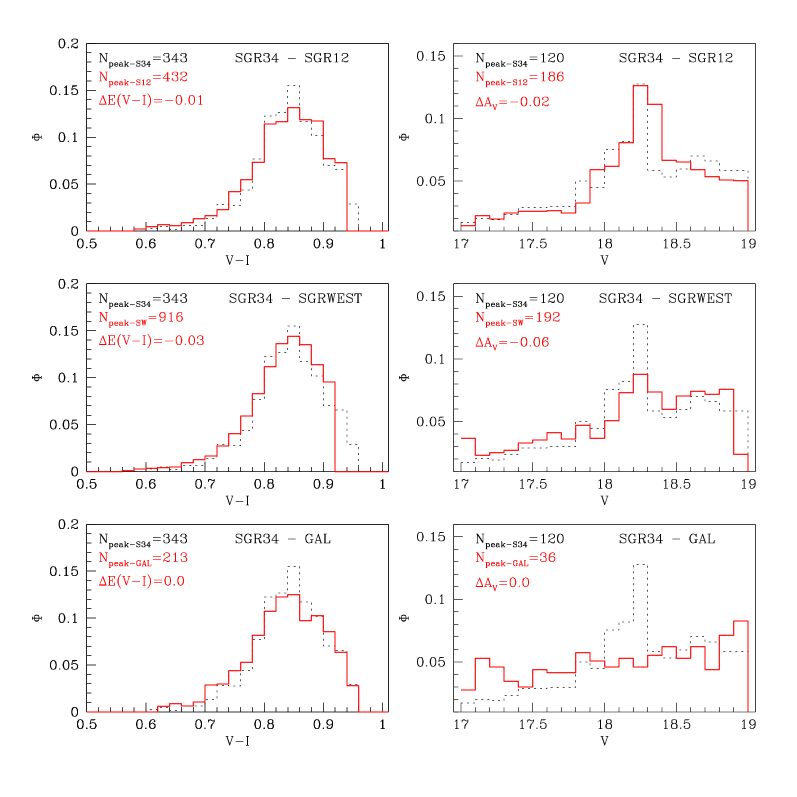
Figure 9: Differential reddening between SDGS Fields. Histograms in color (left panels) and in V magnitude (right panels) are presented for the Vertical Blue Sequence (VBS) of the contaminating population and the Sgr HB, respectively. All histograms are normalized to the total number of considered stars. In each panel the histograms obtained in the considered Field (solid line) has been shifted to match the corresponding distribution obtained for the SGR34 Field (dashed line). The applied shifts ($\Delta E(V-I)$ and $\Delta A_{V}=1.93\times\Delta E(V-I)$)in color and magnitude are reported in each panel, together with the number of stars in the most populated bin ($N_{peak}$).

In the case of GAL, the independent check provided by the match between HB peaks is obviously impossible and we are forced to consider only the color distributions of VBSs. We finally adopt $\Delta E(V-I)_{GAL}=0.0$, but this result bear a considerable uncertainty.

Table 2 presents a synoptic view of the reddening estimates for the SDGS Fields (from ASRM, from previous direct measures and the ones obtained above) and for the fields containing Sgr globulars (from literature): Ter 8 ($l^{o}=5.76;b^{o}=-24.56$), Ter 7 ($l^{o}=3.39;b^{o}=-20.07$), M54 ($l^{o}=5.61;b^{o}=-14.09$) and Arp 2 ($l^{o}=8.55;b^{o}=-23.27$). All estimates are consistent with no (or very little) reddening differences across the region of the Sgr dSph sampled by SDGS. Interstellar extinction appear rather homogeneous also on the wider scale covered when directions toward Sgr GCs are also considered ($\sim 10~{}deg$ across).

Table 2: Reddening estimates for SDGS Fields and Sgr GCs.

Field		E(V-I)
	ASRM∗	Direct Estimates	SDGS⋆
SGR34	$0.20\pm 0.01$	$0.22\pm 0.04^{1}$	$0.22\pm 0.04^{2}$
SGR12	$0.24\pm 0.01$	$0.21\pm 0.03^{3}$	$0.23\pm 0.05$
SGRWEST	$0.22\pm 0.01$	—	$0.25\pm 0.05$
GAL	$0.14\pm 0.02$	—	$0.22\pm 0.06$
M54	$0.24\pm 0.04$	$0.21\pm 0.03^{3}$	—
Ter 8	$0.22\pm 0.04$	$0.19\pm 0.05^{4}$	—
Ter 7	$0.14\pm 0.02$	$0.11\pm 0.05^{5}$	—
Arp 2	$0.17\pm 0.03$	$0.16\pm 0.03^{5}$	—

5 Population differences between the three Fields

While detailed studies of the age and metallicity of Sgr populations needs accurate decontamination of the samples from foreground stars, many useful statements can be made on the CMDs presented in fig. 5, 6, and 7. In particular we used the wide spatial coverage of SDGS to search for possible differences in the Sgr stellar content in different regions of the galaxy.

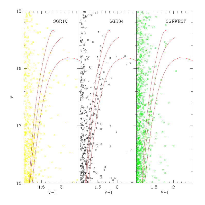
Figure 10: The giant branch of the Sgr Pop A in the three SDGS Fields. SGR12 and SGRWEST stars were corrected for differential reddening with respect to SGR34, according to the values found in sect. 4.1.1. The solid lines are the mean RGB loci for three galactic globular cluster (from right to left): 47 Tuc ($[Fe/H]=-0.71$), NGC1851 ($[Fe/H]=-1.29$) and NGC 6752 ($[Fe/H]=-1.54$), from DCA1990. The ridge lines have been reported to the same distance of Sgr (assuming $V_{HB}(Sgr)=18.22$) and reddened in order to match the reddening of SGR34.

5.1 Constraints on metallicity from the RGB location

Fig. 10 shows a zoomed view of the CMD containing the brightest part of Sgr RGB in the three SDGS Fields (SGR12, left panel; SGR34, central panel; SGRWEST, right panel). The small differential reddening corrections described above have been applied to SGR12 and SGRWEST samples to report them to the same reddening as SGR34. For $V<17$ and $V-I>1.3$ field contamination is not a major concern, Sgr RGB clearly stand out, being one of the key feature which led to the discovery of the Sgr galaxy (see IGI-I and IGI-II).

The solid lines in fig. 10 are RGB ridge lines of (from right to left) 47 Tuc ($[Fe/H]=-0.71$), NGC1851 ($[Fe/H]=-1.29$) and NGC 6752 ($[Fe/H]=-1.54$), from Da Costa & Armandroff 1990, shifted at the Sgr distance and reddening.

The most remarkable feature of fig. 10 is the wide color spread of the brightest part of the RGBs, a feature commonly interpreted as indication of significant abundance spread among stars (MUSKKK, SL95, MAL). Any possible spread induced by photometric stochastic errors (few hundredths of mag) should have a negligible effect since it is much smaller than the observed color spread.

The superimposed ridge lines (the same used also by MUSKKK - a further confirm of the excellent agreement between SDGS and MUSKKK photometries) seems to nicely bracket the observed distributions and it can be concluded that the metallicity spread is of order $0.7-0.8~{}dex$. Such spread is rather large with respect to what found in other dSph galaxies [Ursa Minor (Olzewski & Aaronson 1985), Draco (Grillmair et al. 1998), Carina (Smecker-Hane et al. 1994)].

In the left panel of fig. 10 (SGR12) a few stars around ($V\sim 16.5;~{}V-I\sim 2$) suggest the possible presence of an additional RGB sequence significantly more metal rich than 47Tuc, which has no counterpart in the other panels. Such an evidence, if confirmed, would support the claims (based on rather marginal clues) by SL95 and MAL for the possible presence of a slight metallicity gradient toward the center of density of Sgr. Further evidences in favor of this hypothesis will be given below.

5.2 The Horizontal branch

As previously noted, a predominantly red HB around $V\sim 18$ and $V-I\sim 1$ can be easily identified in the CMD in fig. 5, 6, 7. Moreover the signature of this features clearly emerges from star counts over the foreground contamination (see fig. 9). In this section we will determine the mean level and the spread (in V magnitude) of the HB.

The HB dispersion is (potentially) an important observable in this case since it is the result of many factors (photometric errors, evolutionary effects, mix of HB stars of different metallicities) the main one being perhaps the extension of the Sgr galaxy along the line of sight (see IGWIS). Furthermore, also major features in the HB color distribution can probably be depicted out of the confusion produced by foreground star contamination. The left panels of fig. 11 show the V histogram of the box ($17.4<V<18.6;~{}0.95<V-I<1.15$) which presumably contain the region of the Sgr HB less affected by contamination (i.e. the red part). RR Lyrae stars, probably present in our sample but with V and V-I measured at random phase, lie in a region of the CMD where many foreground stars are also found. Comparison of the upper three panel of fig. 11 with the lower one (GAL, corrected for the factor accounting for the smaller sampled area) clearly states that Sgr population is largely dominant in this box. An evident bell shaped distribution is present between $V\sim 18$ and $V\sim 18.5$: we compute the mean V magnitude ($<V_{HB}>$) and standard deviation ($\sigma_{V_{HB}}$) over this range for the SGR12, SGR34, and SGRWEST samples. The results are reported in table 3, together with $3\sigma$ errors on the mean ($3\sigma_{V_{HB}}/\sqrt{N_{star}}$) that we take as conservative error on the $<V_{HB}>$ estimates. All $<V_{HB}>$ and $\sigma_{V_{HB}}$ estimates are consistent within the errors. In the last row of table 3 are reported the average values over the three Fields, calculated after the application of the differential reddening correction to SGR12 and SGRWEST with respect to SGR34. The mean value is $<V_{HB}>=18.22\pm 0.02$, consistent within errors with all previous estimates (MUSKKK, MAL, LS97). A particularly good agreement is achieved with SL95 ($<V_{RHB}>=18.25\pm 0.05$, for the red HB) and IGWIS ($<V_{HB}>=18.25\pm 0.05$, from their fig. 2). The $<V>_{RRLyrae}=18.16\pm 0.05$ estimate obtained by MUSKKK from a small sample of RR Lyrae variables toward SGR34 seems marginally inconsistent with our estimate, above all if it is taken into account the fact that RR Lyrae are expected to be slightly fainter than very red HB stars (see DCA90, for example) at the same metallicity. However, two out of seven of the MUSKKK RR Lyrae are much brighter than the mean HB level (see their fig. 2) and have probably a great weight on the final average $<V>_{RRLyrae}$ value. A deeper analysis of the RR Lyrae sample of MUSKKK is performed by MKSKKU. The average of the bona fide RR Lyrae from table 8 of MKSKKU (i.e. SV1, SV2, SV3, SV4, SV6 and SV7) gives $<V>_{RRLyrae}=18.26\pm 0.05$, in agreement with our result. Furthermore it must be considered that red HB stars and RR Lyrae in Sgr almost certainly have NOT the same metallicity, so comparisons are significant only in a rough sense. Finally, Mateo et al. (1996) found $18.22\leq V_{RRLyrae}\leq 18.36$ for 3 RR Lyrae associated to Sgr in the line of sight toward M55.

At present it is not possible to disentangle the different factors contributing to the magnitude dispersion of the HB stars. The only firm conclusion that can be drawn at the moment is that $\sigma_{V_{HB}}$ is clearly larger than photometric error at that magnitude.

Table 3: HB levels and dispersion for SDGS Fields.

Field	$<V_{HB}>~{}\pm 3\sigma_{V_{HB}}/\sqrt{N_{star}}$	$\sigma_{V_{HB}}$
SGR34	$18.23\pm 0.02$	$0.12$
SGR12	$18.26\pm 0.02$	$0.12$
SGRWEST	$18.25\pm 0.02$	$0.13$
average†	$18.22\pm 0.02$	$0.12\pm 0.01$

^† After corrections for differential reddening.

5.2.1 Distance Modulus

A straightforward way to determine Sgr distance from $<V_{HB}>$ is to find the differential distance modulus with respect to a well studied globular cluster of comparable metal content and HB morphology. The ideal subject in this case seems to be 47 Tuc, the prototypical metal rich globular. First of all we correct for interstellar extinction the average $<V_{HB}>$ value, obtaining $<V_{HB}>_{0}=17.80\pm 0.05$ for Sgr. Adopting for 47 Tuc, $<V_{HB}>_{0}=14.06$ and $(m-M)_{0}=13.51$ from DCA90 we obtain:

$$\Delta(V_{HB})=V_{HB}(Sgr)-V_{HB}(47Tuc)=3.74$$

and finally:

$$<(m-M)_{Sgr}>_{0}=17.25^{+0.1}_{-0.2}$$

corresponding to $\sim 28^{+2}_{-4}Kpc$

The asymmetrical error bar is due to the correction made by DCA to account for the expected higher luminosity of 47 Tuc red HB stars with respect to RR Lyrae, on which their distance scale is based. They assume that HB stars of 47 Tuc are 0.15 mag brighter than RR Lyrae. While correction of this amount are commonly used the uncertainty on the actual value is comparatively large, since correction of $\sim 0.05$ mag have also been suggested. Taking into account the large uncertainty in this correction (that was never considered before in deriving the distance to the Sgr dSph ; see IGWIS, MUSKKK, MKSKKU) it can be useful to provide also an estimate of distance modulus without the DCA90 correction, i.e.: $(m-M)=17.1\pm 0.2$($\sim 26\pm 3Kpc$), in good agreement with published measures (IGWIS, MUSKKK, MKSKKU). However, it has to be stressed that some correction is necessary to report the mean level of the red HB to the mean level of RR Lyrae as is apparent from fig. 6 of MKSKKU. The marginal disagreement between our estimate (corrected for the quoted effect) $(m-M)_{0}=17.25^{+0.1}_{-0.2}$ and the distance modulus derived by MKSKKU $(m-M)_{0}=17.02\pm 0.19$ is due do the different extinction law assumed. In fact, from the same $E(V-I)=0.22\pm 0.04$ they derive $A_{V}=0.55$ while in the present work $A_{V}=0.42$ is assumed, according to RL.

Finally we recall that while the error on the estimate by MKSKKU take into account also the uncertainty on the slope of the $M_{V}(RRLyrae)~{}vs.~{}[Fe/H]$ relation, our error bar do not include this effect.

Figure 11: Histograms in magnitude (left panels) and color (right panels) for the stars in the HB box (see text). Comparing the two upper-right panels (SGR34 and SGR12, respectively) the redder morphology of the HB in SGR12 is evident: a clear bump is present at $V-I\sim 1.07-1.10$ which has no counterpart in the SGR34 and SGRWEST histograms.

5.3 HB morphology

The right panels of fig. 11 report the color distribution of stars in the HB box described above. While HB stars distribution seems very flat in this range of colors for SGR34 and SGRWEST, the histogram of the SGR12 sample presents a clear bump at $V-I\sim 1.07-1.10$ having no counterpart in the SGR34 and SGRWEST histograms. SL95 argued for a “double” HB morphology of Sgr stars in this region: a Red Clump HB, that they associate with a population 10 Gyr old and with $[Fe/H]\sim-0.5$, plus an “ordinary ” red HB associated with an older and more metal poor ($[Fe/H]\sim-1.3$) population, similar to globular clusters like NGC 362, Pal 4 and Eridanus.

SGR12 color histogram of fig. 11 seems to support this view. In particular, the presence of a second peak at $V-I\sim 1.02-1.04$ may suggest a true bimodality of the HB morphology. However the significance of the apparent bimodality cannot be firmly established at present, and has to be regarded as a marginal evidence, at least unless accurate decontamination have been carried on (Paper II).

On the other hand the detected difference in HB morphology between SGR12 and SGR34 and SGRWEST is very likely to be real. A Kolmogorov-Smirnov test states that the probability that SGR12 and SGR34 HB samples are drawn from the same parent population in color is less than $3\%$. Note that the presence of the nearly uniform contaminating population in this region of the CMD tend to smear out real differences in the distributions of Sgr stars, so the above figure can be regarded as a strong upper limit for likelyhood of the quoted null hypothesis. This results are unaffected if the SGR12R sample, instead of the whole SGR12 one, is used.

The redder HB morphology coupled with the redder RGB discussed in sec. 5.1 suggest the presence of a metallicity (and age?) gradient from the outer regions toward the center of density of the Sgr dSph (SGR12).

5.4 Number counts comparisons

In the previous sections we presented CMDs based on large samples of stars measured in three different region of the Sgr galaxy. The samples are populous enough to be representative of the stellar population in each region of the galaxy. In order to put in evidence (quantitatively) possible spatial differences in stellar content among the surveyed Fields we compared star counts in selected boxes in the CMDs. The boxes have been defined to select regions of the CMDs dominated by one clear-cut feature, and so they are expected to track unambiguously only one of the stellar components identified on the SDGS CMDs (i.e. Sgr Pop A, Sgr Pop B or Milky Way Bulge+disc).

We identified five key features on the CMD. Three of them (the Sgr RGB, the red HB around $V\sim 18$ and the upper Main Sequence around $V\sim 21$ and $V-I\sim 0.75$, just above the TO point) have been taken as tracers of Sgr Pop A, since are clearly associated with this older population. The fourth selected feature is the Blue Plume described in sec. 3 and associated with Sgr Pop B, and the fifth is a portion of the vertical Bulge+disc sequence, tracing the degree of foreground contamination of the considered Field.

Figure 12: The boxes selected for star counts of tracer populations are represented and labeled, superimposed on the CMD of an arbitrary subsample of SGR34 stars. Only a relatively low number of stars have been plotted to avoid boxes being hidden by ink blobs.

The boxes have been defined in order to avoid reciprocal contamination between the different CMD features. . The boxes, labeled after the dominant population sampled, are clearly illustrated in fig. 12 and are defined as follows:

• RGB: $16.0\leq V\leq 17.8$ and $1.25\leq V-I\leq 1.7$ containing most of the Sgr Pop A Red Giant Branch.

• HB: $18.0\leq V\leq 18.5$ and $0.95\leq V-I\leq 1.2$ containing most of the Sgr Pop A Horizontal Branch, at least the part less affected by the contaminating sequence.

• TO: $21.0\leq V\leq 21.5$ and $0.65\leq V-I\leq 0.8$ around the brightest part of Sgr Pop A Main Sequence, just above the Turn Off point. In this case we can take advantage of the high number of stars in this region of the CMD to minimize the dimension of the box without any loss in statistical significance. So, the box edges are chosen with particular care to avoid contamination from the large number of foreground/background sources present in the CMD for $V-I>0.9$ at this magnitude level. The significance of star counts in this box is nevertheless seriously weakened by two factors: (a) the completeness is less than $50\%$ for $V\sim>21.$ in each of the SDGS Fields, so the completeness correction is very large and uncertain; (b) the completeness factor is not well defined at that magnitudes for the SGR12 and GAL samples, the faint edge of the box being very near to the detection threshold of the photometry. Star counts in the TO box for these Fields must be considered only as lower limits. However SGR34 and SGRWEST have very similar completeness and limiting magnitude, so number counts comparisons between these latter samples is probably significant and very interesting.

• BP: $18.8\leq V\leq 21.$ and $0.2\leq V-I\leq 0.6$ containing most of the Blue Plume sequence (Pop B). The faint edge of the box is close the $C_{f}=0.5$ limit, so some underestimation in star counts for SGR12 and GAL (see above) can be expected.

• BMS: (Bulge Main Sequence) $18.6\leq V\leq 19.5$ and $0.75\leq V-I\leq 0.95$. The box select the foreground star sequence in a zone of the CMD where the completeness is fair and the expected contamination by Sgr stars is virtually null.

Table 4: Star counts in selected CMD boxes.

Field	$N_{RGB}$	$N_{HB}$	$N_{TO}$	$N_{BP}$	$N_{BMS}$
GAL	34	200	283*	154	1357
SGR34	105	430	2940	306	1235
SGR12	160	756	2670*	648	2183
SGRWEST	140	753	1784	457	4940

* asterisks indicate uncertain values (see text)

For the star counts in the RGB and HB boxes the whole SGR12 sample was used, while for the boxes below $V=18.5$ (TO, BP and BMS) the SGR12R sample was adopted, in order to prevent misleading effects from the modest quality of the photometry at faint magnitudes of subfields SGR12D and E (see sec. 2). Star counts from the SGR12R and GAL sample have been normalized to the area of a whole strip ($\simeq 9\times 35~{}arcmin^{2}$), multiplying the observed number counts by a 5/3 factor. All the counts were corrected for completeness according to the relations shown in fig. 3.

The corrected number counts in the different boxes are reported in table 4 and displayed in fig. 13 for GAL and for the Sgr Fields ordered with increasing galactic latitude (labels with the approximate latitude of the Sgr SDGS fields are also reported). The error bars have been obtained applying error propagation, adding Poisson 1-$\sigma$ uncertainties in number counts to an assumed conservative error of $10\%$ in the applied completeness corrections.

The upper four panels of fig. 13 should be interpreted with some caution, since, as we will show below, the contamination of star counts by foreground stars can be very different from Field to Field. However some general features are readily evident:

1. Star counts in boxes containing tracers of Sgr population (RGB, HB, BP and TO - upper four panels) are significantly higher in Sgr Fields with respect to GAL.

2. The trend of star counts with galactic latitude is remarkably similar for the upper three panels of fig. 13, the first two reporting tracers of Sgr Pop A and the third reporting a Pop B tracer.

3. Star counts in the TO box are significantly higher in SGR34 than in SGRWEST. The dashed square around the point representing TO star counts in SGR12 has the aim of emphasizing the large uncertainty affecting this estimate (see above). The true $N_{TO}(SGR12)$ could be significantly higher than what reported.

Figure 13: Number of stars counted in the selected boxes (see fig. 12) for each SDGS Field plotted as a function of galactic latitude. The dashed square around $N_{TO}$ for the SGR12 Field indicate that this number should be considered as a lower limit.

However, the most important result of fig. 13 resides in the lowest panel, reporting star counts in the CMD box tracing the sole contaminating population. The very steep gradient in the number of foreground stars between $b=-16^{o}$ and $b=-12^{o}$ can be quantitatively appreciated: this number nearly doubles from the position of SGR34 to that of SGR12, and it roughly doubles again from SGR12 to SGRWEST. Furthermore it result evident that the GAL Field represents optimally the contaminating population for SGR34 while it significantly underestimates contamination for SGR12 and SGRWEST. This latter fact must be taken into account also when CMD statistical decontamination is attempted (SDGS Paper II).

5.5 Decontaminating star counts

Ideally, one can effectively remove much of the contamination in star counts by subtracting the star counts in a given box of a CMD containing only stars belonging to the Contaminating Population (CP) to the star counts in the same box of a CMD containing Sgr+(CP) stars, once a sample with the following characteristics is available:

1. composed solely of CP stars

2. representative of the CP present in the CMD containing both Sgr and CP stars (i.e., same CP star density in each box).

In order to quantify how much the GAL sample is representative of the CP in the different SDGS Fields we defined the ratio

$$\phi_{SgrField}=N_{BMS}(SgrField)/N_{BMS}(GAL)~{}~{}~{}~{}.$$

This index approximatively represents the degree of contamination in each Field with respect to the GAL field. It is obtained: $\phi_{SGR34}=0.9$, $\phi_{SGR12}=1.6$ and $\phi_{SGRWEST}=3.6$.

So, it can be concluded that the GAL sample seems fairly representative of the CP in SGR34 (see also fig. 13, lower panel).

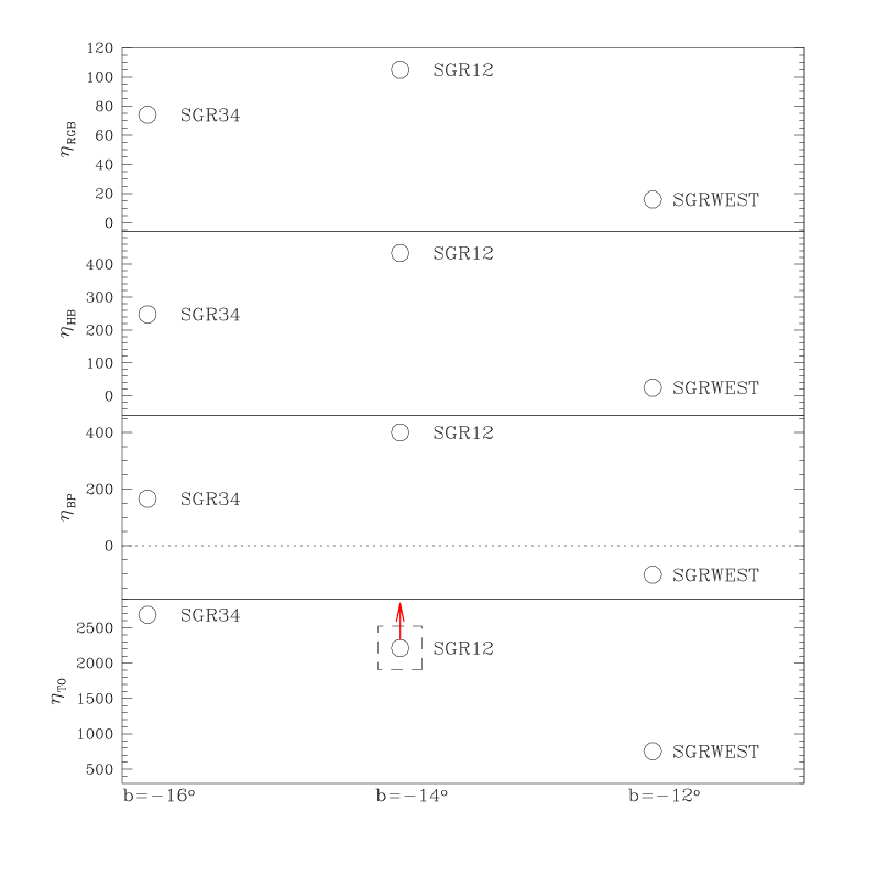
Figure 14: The same as figure 13, for decontaminated star counts (see text). The arrow indicates that the reported $\eta_{TO}(SGR12)$ is a lower limit.

Furthermore, we can use the $\phi$ ratio to estimate the expected number of CP star in a given box for the SGR12 and SGRWEST samples.

By multiplying the number of star in a given box in the GAL sample by the appropriate $\phi$ ratio we can obtain such estimate, and then subtracting it to the counts in the same box of the CMD of a Sgr Field we get the number of Sgr stars in that box for the given Sgr Field. Let’s call this number $\eta_{box}(SgrField)$, defined as follows (taking as an example the HB box and the SGR34 Field):

$$\eta_{HB}(SGR34)=N_{HB}(SGR34)-[N_{HB}(GAL)\times\phi_{SGR34}]~{}~{}~{}.$$

where the term included in the square brackets is an estimate of the number of CP stars present in the HB box of the SGR34 CMD and $\eta_{HB}(SGR34)$ is in principle, the number of true Sgr stars in the HB box of the SGR34 CMD.

We can reasonably expect that passing from $N_{box}$ to $\eta_{box}$ much of the contamination is removed. Given the strong gradient of CP star density in the region of sky occupied by Sgr dSph , the adopted approach is the most viable to deal with Sgr star counts. The only alternatives coming to mind are:

1. to estimate the degree of local contamination by adopting a Galaxy model [as, for example, Bachall & Soneira (1980, 1984)]. However this approach is prone to large uncertainties when applied to such small spatial scales.

2. To acquire a large number of control fields in different positions (for example, a sequence of fields along a line parallel to Sgr major axis, some degree apart) such to have a significant probability to get representative CP samples for each of the Sgr fields to analyze. This strategy is very expensive in terms of observation time and still the “degree of representativity” must be somehow estimated “a posteriori”.

As correctly pointed out by the referee, the main pitfall of the adopted approach resides in the implicit assumption that the latitude density gradient of bulge and disc stars is similar (in the considered range, i.e. from $b=-16^{o}$ to $b=-12^{o}$) or, in other words, that the CMDs of the CP stars in the different fields differ only in the number of stars. This is indeed a rather crude approximation that could introduce significant systematic errors in the “decontaminated” number counts. This possible occurrence has to be taken into account while interpreting the results presented in the following subsections (sec. 5.1.1 and 5.1.2).

The caveats described in the previous section concerning $N_{TO}$ obviously apply also to $\eta_{TO}$, in particular for the SGR12 sample.

The plots $\eta_{box}~{}vs.~{}Sgr~{}Field$ are displayed in fig. 14. Labels and symbols are the same as fig. 13, obviously without the GAL points since, by definition, $\eta_{box}(GAL)=0$ for any box. No error bar is reported since the indeterminacy in the procedure from $N$ to $\eta$ is tied only to the validity of the assumption of “representativity”, so intrinsically hard to quantify.

5.5.1 Asymmetry in density distribution

The upper two panels of fig. 14 show the behaviour of star count for the most reliable tracers of Sgr Pop A, i.e. $\eta_{RGB}$ and $\eta_{HB}$. The trend is very similar in both panels: there is an enhancement in Sgr stellar density from SGR34 to SGR12 by a factor $\sim 1.6$ while the enhancement between SGRWEST and SGR12 is of nearly one order of magnitude. There are two possible explanation for this fact: (1) the tidal limit of the Sgr dSph occurs at lower galactic latitudes with respect the SGRWEST Field (i.e. the field is devoid of Sgr stars), or (2) there is a clear asymmetry in the distribution of Sgr stars along the major axis, the region nearer to the Galactic Bulge suffering strong star depletion (possibly related to ongoing disruption by tidal interaction with the Galaxy). The first hypothesis is ruled out by the lower panel of fig. 14: $\eta_{TO}(SGRWEST)=754$, so there is a clear excess of stars in the TO box of SGRWEST with respect to GAL. Then, it must be concluded that Sgr stars are still significantly present at $b=-12^{o}$ (as already stated by IGWIS) but the Sgr star density is probably much lower with respect to the symmetrical SGR34 Field [see also the comparison between $\eta_{TO}(SGRWEST)$ and $\eta_{TO}(SGR34)$] and there is no symmetry in star distribution with respect to the center of density ($\sim$ SGR12), at least along the major axis.

The decreasing in star counts from the SGR12 Field to the SGR34 Field is in rough accord with what expected for a King Model distribution (assuming $C\sim 0.5$, $r_{t}\sim 4^{o}$ and $r_{c}\sim 1.25^{o}$, as estimated by IGWIS) but the strong star deficiency in SGRWEST seems to rule out King Models as viable density distributions for Sgr. The clumpy nature of the Sgr galaxy has already been noted [IGI-II, IGWIS, Mateo et al. (1996)] and the SGR34 Field is centered on one of the main subclump (IGI-II). However the fall of star counts toward SGRWEST is very steep and suggest a remarkable depletion of Sgr stars in this region.

We recall again that decontaminated star counts can be affected by unaccounted variations in the CP composition from field to field. On the other hand, it has to be considered that the same result is found from star counts in very different regions of the CMD. One would expect that the various windows (TO,HB,RGB,BP) have to be affected in different ways if the distribution of CP stars in the CMD changes significantly from $b=-16^{o}$ to $b=-12^{o}$. So, while the actual extent of the asymmetry is quite uncertain, it seems unlikely that differences in the relative abundance of bulge and disc stars could produce such an effect in all the selected windows.

5.5.2 The distribution of the Blue Plume population

If the Blue Plume stars are associated to a younger generation of stars (Pop B) their distribution in the galaxy may be very different from the main population. Presently active dwarf galaxies are observed to experience very localized burst of star formation on scales of the order of few $\sim$ 100 pc (Tosi 1993, Hunter 1998), significantly smaller than the scale sampled by SDGS, ($\sim 2~{}Kpc$ from SGR34 to SGRWEST). The third panel (from up to down) of fig. 14 shows that this is not the case for Sgr, the general behaviour of $\eta_{BP}$ remarkably resembling the trend of the Pop A tracers $\eta_{RGB}$ and $\eta_{HB}$, at least in the transition from SGR34 to SGR12.

On the other hand $\eta_{BP}(SGRWEST)=-103$, i.e. the contribution by the contaminating population in this box is expected to be higher than actually observed in the SGRWEST Field. This result is ambiguous since can indicate that (a) the BP population is absent in this region, or (b) the number of BP stars is too low to survive the decontamination because of the low density of Sgr in this region. We put it in evidence since, in our view, it surely deserves further check ( a deeper photometric study or a survey of bright Pop B tracers, as Carbon Stars).

Finally we can try to roughly estimate the contribution of Pop B stars to the whole Sgr population. The most suitable sample for this purpose is SGR34. The factor $f={\eta_{BP}\over{{(\eta_{TO}+\eta_{BP})}}}\simeq 0.06$ can be taken as an upper limit for the relative contribution of BP stars in this Field.

6 Is there a metal poor (and old) population in Sgr?

The only direct evidence of the presence of a (relatively) old and metal poor population in the Sgr dSph comes from the detection of RR Lyraes (MUSKKK, Mateo et al 1996, Alcock et al. 1996). As pointed out by IGWIS, the mere existence of such stars is indicative of age $\sim>10-12~{}Gyr$ and metallicity $[Fe/H]\sim<-1.5$. However, at least two member of the Sgr globular cluster system are significantly older and more metal deficient than the above figures, i.e. Ter 8 ($[Fe/H]=-2.0$ see MoAL, Da Costa & Armandroff 1995) and M54 ( $[Fe/H]=-1.79$, see MAL and SL97). So, if the formation of GCs is not completely decoupled from the star formation in the host galaxy (i.e. Ter8 and M54 formed many Gyrs before the onset of star formation in Sgr), some fraction of stars with age and metallicity similar to the above quoted globulars should be present also in the Sgr field. This hypothesis can be tested looking in the CMDs for features typical of old and metal poor globular clusters. In particular we used the mean loci defined by stars in the CMD of Ter 8 to test if a “Ter 8-like” population is present in the Sgr galaxy. We adopted the ridge line by MoAL, since the instrumental set up of MoAL is the same used for the SDGS.

Figure 15: The Ter 8 ridge line (by MoAL) is superposed to the CMD of a subsample of stars in the SGR34 Field, after the corrections specified in the text.

The SDGS and MoAL CMDs were corrected for reddening and a shift $\Delta V_{0}=+0.25$ were applied to the Ter 8 ridge line in order to roughly match HB levels. This shift correspond to reporting Ter 8 to the average distance of Sgr, since the cluster seems to lie slightly in foreground along the line of sight with respect to the main body of the host galaxy (see IGWIS and Da Costa & Armandroff 1995). The correction takes into account also the expected difference between the level of the very blue HB (Ter 8) and the stubby red one of the Sgr dSph (see sec. 5.2.1).

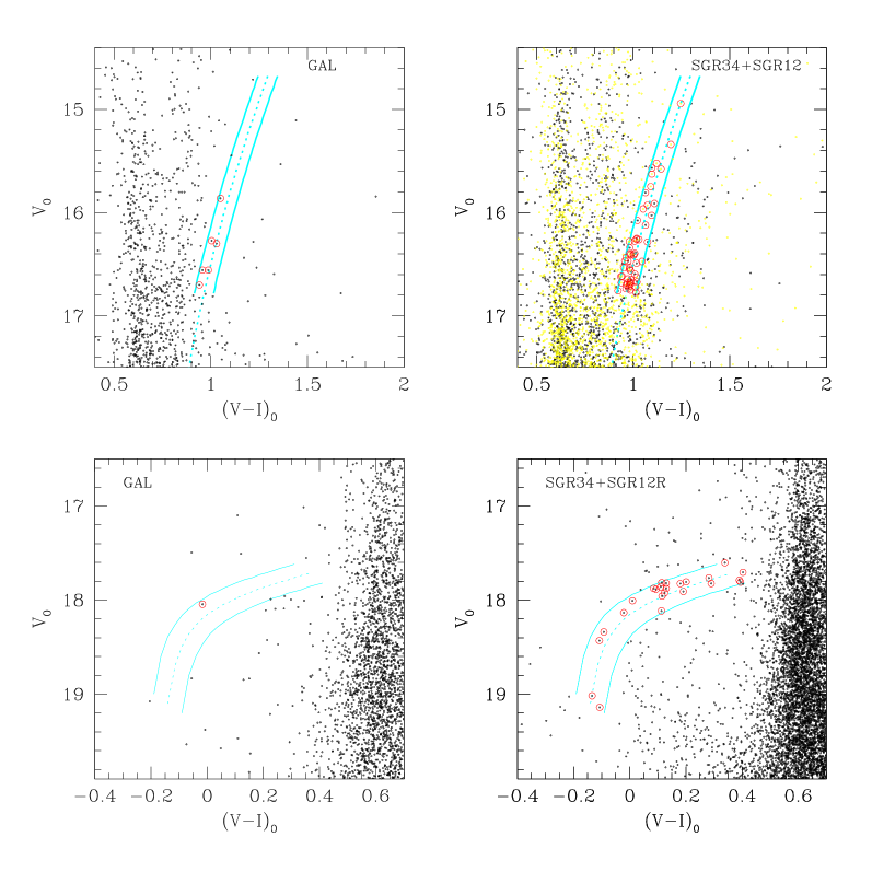
Figure 16: The RGB and HB mean ridge lines (dashed line) of Ter 8 (by MoAL) overplotted on the CMD of the GAL Field (left panels) and of the SGR34+SGR12 Fields (right panels). Solid lines represent $\pm 0.05$ color edges with respect to the mean ridge lines. Stars lying in the strips are put in evidence by open circles. The samples actually adopted in each case are also indicated.

In fig. 15, the Ter 8 ridge line is superposed to the SGR34 CMD. Two main features of the Ter 8 population can be unambiguously identified in the SDGS CMDs, clearly emerging from the sequences formed by either Sgr and CP stars: the brightest part of the RGB (between the redder Sgr RGB and the CP sequences, above $V_{0}\sim 16.5$; hereafter T8RGB) and the blue HB tail around $V_{0}\sim 18.2$ and between $-0.2\leq(V-I)_{0}\leq 0.4$ (hereafter T8HB). The excess of stars around this features in the Sgr Fields CMDs, with respect to the control GAL sample, can be considered as a signature of the presence of a “Ter 8 - like” population.

In fig. 16 the location of the Ter 8 ridge line (dashed line) is reported on the GAL (left panels) and on the SGR34+SGR12 CMDs (right panels). Upper panels shows the RGB region and lower panels show the blue HB region. The continuous lines represent $\pm 0.05$ edges (in color), with respect to the ridge line. Stars lying in these strips are evidenced by open circles. These stars can be reasonably considered to belong to a Ter 8-like population.

The excess of such stars in the Sgr CMDs with respect to the GAL one is clear from the comparison between right panels and left panels in fig. 16.

However, a truly significant comparisons can be performed only after the correction for the different area sampled by the GAL Field and by SGR34+SGR12 has been applied to star counts in the defined strips (completeness corrections are irrelevant at the considered magnitude levels).

Once the area-normalization has been performed, we can test the null hypothesis that the difference between star counts in the T8RGB and T8HB regions in the SGR34+SGR12 and GAL samples be zero, i.e. the Ter 8 - like stars are associated to the contaminating population and NOT to Sgr. The measured excess in star counts rules out such hypothesis at $4.3\sigma$ level for the blue HB stars and at $3.5\sigma$ level for the T8RGB stars. We are aware that a number of uncertainties can affect this result (small number statistics or errors in the distance moduli, for instance) but a casual star count excess in two independent strips would be a too unlucky coincidence. Furthermore, the same procedure was also applied to the MAL and MUSKKK CMDs and fully consistent results have been found. The application of the test to the SGRWEST sample is a risky task because of (a) the very high degree of foreground contamination in this Field and (b) the relatively low number of Pop A Sgr stars, whose the searched population is a further subsample. Despite these drawbacks a slight Ter 8 -like star excess is found also in SGRWEST.

We take the above result as the first direct identification of very metal poor stars in the Sgr dSph galaxy. Direct spectroscopic follow-up of a consistent sample of T8RGB stars can confirm or rule out this claim by simultaneously determining (i) the membership to Sgr, via radial velocity estimates and (ii) the metal content through suitable metallicity indexes measurements. Associating an old age (Ter 8 -like) to the detected metal poor population seems a very reasonable extrapolation, but cannot be directly supported by SDGS CMDs, at this stage.

Finally by counting the number of Sgr RGB stars redder than the T8RGB strip but confined in the same magnitude range, a rough estimate of the relative abundance of Ter 8 -like stars in Sgr can be obtained. It turns out that, with the above assumptions, nearly $\sim<30\%$ of Sgr RGB stars can be associated with the metal poor component, not inconsistent with the large number of RR Lyrae stars probably associated with Sgr (MKSKKU, Alard et al. 1996, Alcock et al. 1996, Mateo et al. 1996, Lepri et al. 1997). Note that candidate RR Lyraes has also been found in Ter 8 (MoAL).

We hope that statistical decontamination on CMDs can help providing stronger constraints on this subject, but the small number of involved stars is not promising, in this sense.

7 Summary and Conclusions

We have described the main characteristics of a large photometric survey (SDGS) devoted to the study of stellar populations in the Sgr dSph galaxy. The power of the SDGS approach is to couple deep and accurate CCD photometry of large samples to a wide spatial baseline.

The analysis presented in this paper (Pap I) was aimed to establish the fundamental properties of the collected samples as internal homogeneity within Fields, the amount of interstellar reddening, completeness etc., that will be at the base of future detailed study of the statistically decontaminated SDGS CMDs (Pap II). Pap II will primarily deal with age and metallicity of the Sgr stellar populations.

A preliminary analysis of the most evident CMD features has also been carried on. Furthermore we performed many test performing a local decontamination from foreground star contributions in small regions of the CMDs. In our view, the adopted technique is complementary to statistical decontamination of the whole CMD (Pap II). The latter is the ideal tool to study the shape of the observed sequences (i.e. for the unambiguous identification of the TO point and to derive safe ridge lines, for example), while the former is more useful to estimate the degree of contamination in the various fields and to put in evidence the main differences in the spatial distribution of stellar components.

In the following, the most interesting results are shortly described and discussed.

• Metallicity spread and gradient: the observed color spread of Sgr RGB stars indicate a wide range of metal content, from $[Fe/H]\sim-1.5$ to $[Fe/H]\sim-0.7$. At present, this is the stronger element witnessing the presence of a mix of stellar populations in Sgr Pop A.

  Both RGB and HB morphology suggest the presence of a more metal rich component in the central region of the galaxy (SGR12), confirming previous claims about a metallicity “radial” gradient in Sgr (SL95, MAL). An association of the very red HB present in the SGR12 field with a young population [instead of (or together with) one with a higher metal content] cannot be excluded at the present stage.

• Detection of a very metal poor population: through comparison of SDGS CMDs with the ridge line of the CMD of the old and metal poor Sgr globular Ter 8, an excess of stars similar to those of this cluster has been found. These stars have been identified as the Sgr “field” counterpart of the ancient component of the Sgr globular cluster system (see MoAL). The only previous hint for the presence of such a population in the Sgr stellar mix was due to the detection of RR Lyrae stars in the galaxy.

• Density distribution asymmetry along the major axis:

  The SGRWEST region (nearer to the Galactic bulge and the leading head of Sgr along its orbit, according to IGWIS) seems significantly deficient of Sgr stars with respect to SGR34.

  If this result is exact, it would be very difficult to find a physical mechanism other than tidal interaction with the Galaxy that can produce such an asymmetry in the density distribution of Sgr stars, given also the remarkable homogeneity of the stellar content. So, it can be considered as a clue suggesting that the tidal disruption of the Sgr galaxy is currently going on.

  It can be conceived that Sgr stars in the SGRWEST region are unbound from the parent galaxy and are slowly spreading along the Sgr orbital path (Johnston 1998, Irwin 1998).

• Pop A and Pop B stars have similar distributions: if the stars in the Blue Plume identified in the CMDs are associated with a younger population (Pop B) it must be concluded that, or (a) both episodes of star formation (Pop A and Pop B) occurred on large scales, comparable with the dimension of the galaxy itself (i.e. stars were formed everywhere nearly at the same epoch), or (b) a very efficient mechanism for star mixing has been at work in Sgr. The two-body relaxation time for this system is, as expected, much greater than one Hubble time for any reasonable assumption about the structure of the galaxy, so hypothesis (a) seems the most likely.

References

- [1] Alcock C. et al., 1997, ApJ, 474, 217
- [2] Alard C., 1996, ApJ, 458, L17
- [3] Bahcall J.N., Soneira R.M., 1980, ApJS, 44, 73
- [4] Bahcall J.N., Soneira R.M., 1984, ApJS, 55, 67
- [5] Buonanno R., Buscema G., Corsi C.E., Ferraro I., Iannicola G., 1983, A&A, 126, 278
- [6] Burstein D., Heiles C., 1982, AJ, 87, 1165
- [7] Da Costa G.S., Armandroff T.E., 1990, AJ, 100, 162 (DCA90)
- [8] Da Costa G.S., Armandroff T.E., 1995, AJ, 109, 2533
- [9] Fahlman G.G, Mandushev G., Richer H.B., Thompson I.B., Sivaramakrishnan A., 1996, ApJ, 459, L65
- [10] Ferraro F.R., Clementini G., Fusi Pecci F., Buonanno R., Alcaino G., 1990, A&AS, 84, 59
- [11] Grillmair C.J., et al., 1998, AJ, 115, 144
- [12] Hernandez X., Gilmore G., 1998, MNRAS, in press (astro-ph/9802261)
- [13] Ibata R.A., Geraint F., 1998, ApJ, 500, 575
- [14] Ibata R.A., Gilmore G., Irwin M.J., 1994, Nature, 370, 194 (IGI-I)
- [15] Ibata R.A., Gilmore G., Irwin M.J., 1995, MNRAS, 277, 781 (IGI-II)
- [16] Ibata R.A., Wyse R.F.G., Gilmore G., Irwin M.J., Suntzeff N.B., 1997, AJ, 113, 634 (IGWIS)
- [17] Irwin, M.J., 1998, in The Stellar Content of the Local Group, IAU Symp. 192, R. Cannon & P. Whitelock eds., S. Francisco: ASP, in press
- [18] Johnston K.V., 1998, ApJ, 495, 297
- [19] Hunter D.A., 1998, in T. Richtler and J.M. Braun, Eds., The Magellanic Clouds and Other Dwarf Galaxies. in press
- [20] Koribalski B., Johnston S., Optrupceck R., 1995, MNRAS, 270, L43
- [21] Landolt A.U., 1993, AJ, 104, 340
- [22] Layden A. C., Sarajedini A. 1997, ApJ, 486, L107 (LS97)
- [23] Lepri S., Mateo M., Layden A., Lemley S., Olzewski E., Morrison H., 1997, BAAS, 191.8102
- [24] Maraston C., 1998, MNRAS, submitted
- [25] Marconi G., Buonanno R., Castellani M., Iannicola G., Pasquini L., Molaro P., A&A, 330, 453 (MAL)
- [26] Mateo M., Udalski A., Szymansky M., Kaluzny J., Kubiak M., Krzeminski W., 1995a, AJ, 110, 1141 (MUSKKK)
- [27] Mateo M., Kubiak M., Szymanski M., Kaluzny J., Krzeminski W., Udalski A., 1995b, AJ, 110, 1141 (MKSKKU)
- [28] Mateo M., Mirabal N., Udalski A., Szymanski M., Kaluzny J., Kubiak M., Krzeminski W., Stanek K.Z., 1996, ApJ, 458, L13
- [29] Mighell K., Armandroff T., Sarajedini A., Layden A., Mateo M., Fusi Pecci F., Ferraro F., Buonanno R., 1997, BAAS, 190, 35.05
- [30] Montegriffo P., Bellazzini M., Ferraro F.R., Martins D., Sarajedini A., Fusi Pecci F., 1998, MNRAS, 294, 315 (MoAL)
- [31] Fusi Pecci F., Bellazzini M., Cacciari C., Ferraro F.R., 1995, AJ, 110, 1664
- [32] Olszewski E.W., Aaronson M., 1985, AJ, 90, 2221
- [33] Renzini A., 1998, AJ, in press (astro-ph/9802186)
- [34] Rieke G.H., Lebovski M.J., 1985, ApJ, 288, 618 (RL)
- [35] Sarajedini A., 1994, AJ, 107, 618
- [36] Sarajedini A., Layden A., 1995, AJ, 109, 1086 (SL95)
- [37] Sarajedini A., Layden A., 1997, AJ, 113, 264 (SL97)
- [38] Schlegel D.J., Finkbeiner D.P., Davis M., 1997, BAAS, 191, 87.04
- [39] Schlegel D.J., Finkbeiner D.P., Davis M., 1998, ApJ, in press
- [40] Siegel M.H., Majewski S.R., Reid I.N., Thompson I., Landolt A.U., Kunkel W.E., 1997, BAAS, 191.8103
- [41] Smecker-Hane T. A., Stetson P. B., Hesser J. E., Lehnert M. D. 1994, AJ, 108, 507
- [42] Smecker-Hane T. A., Mc William A., Ibata R.A., 1998, BAAS, 192, 66.13
- [43] Stanek K.Z., 1998, ApJ L, submitted (astro-ph/9802093)
- [44] Tosi M., 1993, in P. Prugniel and G. Meylan, Eds., ESO/OHP Workshop on Dwarf Galaxies. ESO, Garching, p. 143
- [45] Walsh J.R., Dudziak G., Minniti D., Zjilstra A.A., 1997, ApJ, 487, 651
- [46] Whitelock P.A., Irwin M., Catchpole R.M., 1996, New Ast., 1, 57 (WIC)
- [47] Zhao H., 1998, ApJ, 500, L149
- [48] Zjilstra A.A., Walsh J.R., 1996, A&A 312, 21
- [49] Zjilstra A.A., Giraud E., Melnick H., Dekker H., D’Odorico S., 1996, ESO Operating Manual n. 15, Version n. 3.0