The time structure of Cherenkov images generated by TeV $\gamma$-rays and by cosmic rays

Abstract

The time profiles of Cherenkov images of cosmic-ray showers and of $\gamma$-ray showers are investigated, using data gathered with the HEGRA system of imaging atmospheric Cherenkov telescopes during the 1997 outbursts of Mrk 501. Photon arrival times are shown to vary across the shower images. The dominant feature is a time gradient along the major axis of the images. The gradient varies with the distance between the telescope and the shower core, and is maximal for large distances. The time profiles of cosmic-ray showers and of $\gamma$-ray showers differ in a characteristic fashion. The main features of the time profiles can be understood in terms of simple geometrical models. Use of the timing information towards improved shower reconstruction and cosmic-ray suppression is discussed.

, , , , , , , , , , , , , , , , , , , , , , , , , , , , , , , , , , , , , , , , , , , , , , , , , , , , , ,

1 Introduction

Imaging Atmospheric Cherenkov Telescopes (IACTs) have become the prime instrument for $\gamma$-ray astrophysics in the TeV energy range, and a number of galactic and extragalactic $\gamma$-ray sources have been established using this technique [1]. Improved understanding of the instruments as well as methodological advances, such as the stereoscopic observation of air showers with multiple Cherenkov telescopes, start to allow precision measurements of source properties, as well as increasingly detailed studies of the relevant characteristics of air showers. During the outbursts of TeV $\gamma$-radiation from the Active Galactic Nucleus (AGN) Mrk 501 in 1997 [4], the HEGRA stereoscopic system of IACTs [2, 3] acquired a large sample of $\gamma$-ray events, ideally suited for such studies by reason of its purity. The analysis presented here makes use of one specific feature of the HEGRA telescopes, namely the recording of the camera signals using fast digitizers, which sample the signal voltages at a frequency of 120 MHz and which allow one to investigate the pulse shapes and the time structure of Cherenkov images. Fig. 1 shows examples of the signals recorded by the telescopes. The detailed investigation of the time structure of images [5] was triggered in particular by the observation of events like the one shown in Fig. 1(b), which exhibit an unusually large time dispersion among the signals observed in different pixels of the IACT camera. Obviously, the timing of pixel signals as well as their amplitude contains information about the evolution of air showers.

Figure 1: Signals recorded by the 120 MHz digitizers of the HEGRA IACT cameras, for two events (a),(b). Signals from all pixels of one camera are superimposed. One time slice corresponds to 8.3 ns.

In the past, the shape and duration of Cherenkov pulses has mainly been investigated using angle-integrating detectors, viewing Cherenkov light from UHE air showers. A seminal review was given by Patterson and Hillas [6], and contains further references. For more recent work, see e.g. [7] and references given there. The HEGRA system of Cherenkov telescopes now allows us to study the detailed time structure of images of TeV cosmic-ray showers and of $\gamma$-ray showers, resolved into individual image pixels of $0.25^{\circ}$ diameter, under conditions where the shower geometry – direction and core distance – is known based on the stereoscopic reconstruction.

The paper is structured as follows: the following chapter introduces briefly the HEGRA IACT system and its performance. Then, the processing of the digitizer signals and the extraction of the amplitude and timing information is described. After a short overview of the data sample used in the analysis, results on the time structure of both cosmic-ray induced showers and $\gamma$-ray induced showers are reported. The paper concludes with a discussion of applications of the timing information towards improving the quality of the shower reconstruction, and the rejection of cosmic-ray showers.

2 The HEGRA IACT system and its performance

The HEGRA IACT system is located on the site of the Observatorio del Roque de los Muchachos on the Canary Island of La Palma, at a height of 2200 m above sea level. The IACT system consists of five telescopes, four of them (CT2,CT4,CT5,CT6) arranged in the corners of a square of roughly 100 m side length, with the fifth telescope (CT3) in the center. Each telescope has a segmented mirror of 8.5 m² area and a focal length of 5 m. During 1997, four of the telescopes (CT3,4,5,6) were equipped with 271-pixel photomultiplier (PMT) cameras, with a field of view of $4.3^{\circ}$ and a pixel size of $0.25^{\circ}$. The fifth telescope (CT2) used an older, coarse-grained camera; this telescope was operated independently of the four identical telescopes. The same is true for the 5 m² prototype telescope (CT1) near the central system telescope.

Due to the relatively modest reflector size and the large focal length, the timing properties of the HEGRA mirrors are excellent, with a maximum time dispersion below 1 ns.

PMT signals of the CT3,4,5,6 telescopes are sampled and digitized every 8.3 ns using 120 MHz Flash-ADCs with an 8-bit dynamic range and a storage depth of 4096 samples. This Flash-ADC memory holds the signal history of the last 34 $\mu s$. To match the bandwidth of the recording system and to suppress frequencies above the Nyquist frequency of the digitizers, the fast photomultiplier signals (about 6 ns fwhm after 22 m of RG 178 cable) are shaped to provide a pulse response $u(t)\sim t\exp{-t/\tau}$, with $\tau=12$ ns. After an air-shower induced trigger, the recording of signals with the Flash-ADCs is stopped and a range of 16 samples is read out for each PMT. The 16 samples are chosen to cover a range from about 50 ns before the arrival of the Cherenkov pulse to about 80 ns after the pulse. Only if the digitized signal exceeds a (software-) threshold of about one photoelectron above pedestal, data for a given channel are stored. This zero-suppression is required to reduce the data volume; however, for monitoring purposes, all channels are read out for every 20th event. The pedestal values for each Flash-ADC channel are updated every two minutes, based on the few Flash-ADC samples recorded before the rising edge of a pulse (time slices 0,1,2 in Fig. 1).

The trigger signal is generated in a two-stage process: a camera trigger signal is generated if the signal in at least two pixels exceeds a preset threshold of typically 6 photoelectrons. The trigger decision is based on the fast, unshaped PMT signals (pulse width 6 ns fwhm). To suppress random coincidences caused by light of the night-sky background, the two pixels have to be direct neighbors. Images of $\gamma$-rays showers are very compact and almost always fulfill this additional condition [8]; the rate of random coincidences, however, is reduced by almost a factor 50. In a second stage, two coincident telescope triggers are required to release a system trigger. Adjustable delays compensate the propagation delays which occur between different telescopes, and which depend on the pointing of the telescopes. Typical rates are in the range of a few 100 Hz to a few kHz for individual pixels, 50 Hz to about 500 Hz for single telescopes, and 15 Hz for the two-telescope coincidence. To serve as time reference marks, both the local camera trigger signal and the global system trigger signal are recorded in a separate Flash-ADC channel of each telescope. The trigger system and its performance is described in detail in [9].

The processing of data involves the extraction of pixel amplitudes as described in the following section, and the definition of images, which include all pixels with a signal above a high ‘tail cut’ of 6 photoelectrons, as well as those pixels above a low tail cut of 3 photoelectrons, which are adjacent to a pixel above the high tail cut. The image centroid is defined as the amplitude-weighted center of gravity of the image pixels, and the image orientation as the major axis of the image ‘tensor of inertia’. Also, the width and length parameters are determined as usual [10].

The image obtained with one telescope corresponds to a view of the air shower in one projection; by combining the different views obtained with the different telescopes, the location and orientation of the shower axis can be determined by simple geometry [2]. The HEGRA telescopes typically determine the orientation of the shower axis event-by-event with a precision of $0.1^{\circ}$. The shower core is located with a resolution of about 10 m, provided that the core is within about 100 m from the central telescope. For larger distances, the core resolution worsens, to about 20 m for 200 m core distance.

The shape of images is used to suppress cosmic-ray showers. Hadronic showers involve larger transverse momenta than electromagnetic showers and generate wider, more diffuse images. To provide a single discriminant, the widths of all images are divided by the width values expected for $\gamma$-ray images, and an average ‘scaled width’ for all telescopes is formed. The expected width for a given telescope depends on the image size (number of photoelectrons in the image), and on the reconstructed distance between telescope and shower core. Other shape parameters are scaled in a similar fashion. With cuts adjusted to accept about 40% to 50% of all $\gamma$-rays, a cosmic-ray rejection factor approaching 100 is possible on the basis of image shapes alone. Cuts based on the pointing of the shower axis [2] provide, for point sources, an additional (multiplicative) rejection factor of the same order.

In the analysis of shower properties, one has to be aware of a potential bias introduced by the criteria chosen to trigger the telescopes and to select the events used in the analysis. The cuts applied here to define $\gamma$-ray candidates are quite loose and accept over 80% of all events, hence a bias is unlikely. The cosmic-ray sample is more strongly biased; the trigger scheme is designed to enhance the fraction of ‘$\gamma$-ray like’ events in the recorded data sample, and some fraction of events is rejected by quality cuts in the stereoscopic reconstruction. According to our simulations, however, the measured properties of cosmic-ray showers are quite representative of the ‘average’ shower.

3 Processing of digitizer signals

A first step in the processing of the Flash-ADC signals is the subtraction of the ADC pedestal; in the next step a digital deconvolution is applied [11], which (partly) reverses the effect of the analog signal shaping. While this shaping is necessary to allow the reliable recording of signals, it does increase the effective integration time and therefore the noise induced by the night-sky background light; the night sky typically contributes 1 photoelectron per 30 ns. In the deconvolution, the new signal $s_{k}$ in the time slice $k$ is calculated as a linear combination of three successive recorded samples $v_{k}$, $v_{k-1}$, and $v_{k-2}$

$$s_{k}=c_{1}v_{k}+c_{2}v_{k-1}+c_{3}v_{k-2}$$

with

$$c_{1}={e^{x-1}\over x},~{}~{}~{}~{}c_{2}=-2{e^{-1}\over x},~{}~{}~{}~{}c_{3}={e^{-x-1}\over x}~{}~{}~{}~{}.$$

Here, $x$ stands for $T/\tau$, with the shaping time constant $\tau=12$ ns and the time interval between samples $T=8.3$ ns. Ideally, a delta-function input signal into the recording chain appears in only two adjacent samples after deconvolution; the ratio of the amplitudes in the two samples measures the arrival time of the signal, relative to the Flash-ADC sampling clock. In reality one usually finds small residual entries in adjacent time slices (Fig. 2(a,b)), indicating either that the pulse shapes are not ideally matched, or that the PMT pulse showed a time spread which is not small compared to the shaping time.

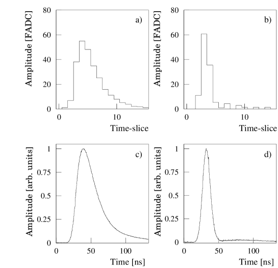
Figure 2: An individual pixel signal before (a) and after deconvolution (b). The average signal shape before and after deconvolution is shown in (c) and (d), respectively, determined by averaging over many signals and different phases relative to the sampling clock, and plotting the mean signal as a function of the time difference between the clock transition and the signal.

A disadvantage of the deconvolution is that the influence of quantization errors is increased. This is particularly relevant, since rather large quantization steps of about one photoelectron have to be used, because of the limited dynamic range of the Flash-ADC system. The benefits of the significantly reduced integration time (Fig. 2) are partly offset by the increased quantization noise, resulting in a net noise of 1.0 photoelectrons in the pixel signal amplitude, with roughly equal contributions from the night sky background, and the electronics noise and quantization.

The arrival time $t$ of the pixel signal is determined based on the center of gravity $q$ of the two adjacent peak samples $s_{k}$, $s_{k+1}$ after deconvolution

$$q={s_{k+1}\over s_{k}+s_{k+1}}~{}~{}~{}.$$

The quantity $q$ is related to (but not identical to) the phase $\phi$ describing the signal timing relative to the Flash-ADC clock. The time $t$ is then given by

$$t=t_{k}+\phi(q)$$

where $t_{k}$ is the time of the clock transition preceeding the signal. In principle, the relation $\phi(q)$ can be calculated on the basis of the signal shape and the deconvolution coefficients $c_{i}$. However, a more reliable approach is based on the fact that for air shower events the arrival times $t$ are random and hence the distribution in $\phi$ has to be flat between 0 and 1. Given the measured distribution in $q$, $f(q)$, one can hence determined $\phi$ using

$$\phi(q)=\int_{0}^{q}f(u)du~{}~{}/~{}~{}\int_{0}^{1}f(u)du~{}~{}~{}.$$

With this definition one determines the mean arrival time of the photons collected in a given pixel, for a given event. This time value is not influenced by amplitude-dependent time-slewing effects, which occur if, e.g., a discriminator is used to define the pixel timing. Detailed Monte Carlo simulations including the response of the PMTs, the signal shaping and the digitization by the Flash-ADC have confirmed that this time determination does reproduce the average photon arrival time at a pixel [12].

Both the relative timing of different pixels as well as the time resolution was determined by illuminating the camera with a pulsed light source (a scintillator excited by ns laser pulses) positioned in the center of the mirror. Small variations in the relative timing of pixels can be caused by differences in the length of signal cables and of clock cables. However, the major effect seen was a dependence of the pixel timing on the high voltage of the PMT (the voltages are adjusted to provide a uniform sensitivity, and vary by up to 300 V between PMTs), see Fig. 3. The time resolution is illustrated in Fig. 4; for signals above 20 photoelectrons, the time resolution is better than 1 ns. The resolution is well described by

$$\sigma_{t}=\sqrt{(0.1\mbox{ ns})^{2}+(4.7\mbox{ ns})^{2}/A}$$

with the pixel amplitude $A$ given in units of photoelectrons.

Figure 3: Mean timing of the light pulser calibration signal, determined for each pixel, as a function of the high voltage applied to the pixel.

Figure 4: Time resolution as a function of the signal amplitude in a pixel, averaged over all pixels.

For each event, the arrival times of the signals in the individual pixels are calculated, and the timing corrections derived using the light pulser signals are applied. A mean arrival time $t_{av}$ for the entire image is then derived by averaging over those pixels which had a signal above the pixel trigger threshold of about 6 photoelectrons. In this average, pixels which overflow the Flash-ADC dynamic range are excluded, as are pixels drawing a significant DC current (e.g., because a star is imaged into the pixel), and pixels with known faults.

It is not unambiguous how to define the pixel amplitude, and two options are provided. In one definition, one scans the deconvoluted Flash-ADC signal for the two adjacent time slices with the maximum sum of amplitudes, within a time window of -8 ns, +20 ns around the mean arrival time $t_{av}$. The amplitude $A_{t}$ is defined as the sum of the two samples. This method has the disadvantage that in particular for very small signals the amplitudes are systematically biased towards larger values, since the selection tends to pick up fluctuations caused by night-sky background or quantization noise.

An alternative definition is to assume that light from the shower will arrive more or less at the same time in all pixels (at least on the scale of the sampling time, $T\approx 8$ ns), and to sum for each pixel the two samples closest to the mean arrival time $t_{av}$, resulting in an amplitude $A_{o}$. This definition results in unbiased amplitudes for synchronous signals, but may cause a loss of signal amplitude in some pixels in the case of a genuine timing dispersion among pixel signals (such as the event shown in Fig. 1(b)). All analyses of HEGRA IACT system data published so far are based on $A_{o}$.

The effective integration time could in principle be further reduced by applying a ‘matched filter’ to the deconvoluted signals, by weighting the two peak samples according to the mean arrival time. For example, in case the arrival time coincides with the clock transition, only a single sample needs to be considered. However, the gain in noise performance is modest and the sensitivity to timing variations is increased further; therefore, this method is currently not used.

Since the deconvolution procedure can only be applied to linear systems, pixels which overflow the Flash-ADC dynamic range have to be handled separately. Overflow recovery is based on the fact that for signals well beyond the dynamic range, the number of samples in the overflow is proportional to the logarithm of the true amplitude. The length of a saturated pulse, or equivalently its area, can hence be used to estimate the true amplitude and to extend the dynamic range. The relation between the area of a saturated pulse and its true amplitude can be calculated from the pulse shape determined with unsaturated pulses. Fig. 5 shows the result of this procedure for overflow recovery; up to amplitudes of 1000 photoelectrons, the spectrum of pulse amplitudes looks undistorted and the spectrum at low pixel amplitudes, where amplitude is directly measured, matches well to the spectrum obtained for large amplitudes after the recovery procedure. Beyond 1000 photoelectrons, nonlinearities in the PMT and in the preamplifier become important, which cannot be corrected in this manner.

Figure 5: Spectrum of pixel amplitudes observed for air showers, for unsaturated signals (lower part of the spectrum), and for saturated signals after recovery (upper part).

Signal amplitudes were so far always quoted in units of photoelectrons. The calibration in units of photoelectrons per ADC count is, however, far from trivial. The method applied to determine the conversion factor is based on the width of the distribution of pixel amplitudes observed with the light pulser system. For a pulser signal containing on average $n$ photoelectrons (with typical values $n\approx 20$ to 150), the width of the amplitude distribution of a given pixel is $\Delta A/A=1/\sqrt{n}$ in the absence of other effects, and one can determine $n$ from this width. In the actual measurements, one has to correct for effects broadening the signal, such as fluctuations in the intensity of the light pulses, fluctuations $\sigma_{spe}$ in the response of the PMT to single photoelectrons, and the (small) smearing due to the variable sampling phase. One finds for the relative width

$$\sigma^{2}={1\over n}+{\sigma_{spe}^{2}\over n}+\sigma_{phase}^{2}+\sigma_{pulse}^{2}~{}~{}~{}~{}.$$

While the first term dominates, there is significant uncertainty in particular in the determination of $\sigma_{spe}$ from laboratory measurements and the resulting calibration factor relating ADC counts to photoelectrons has a systematic error of about 15%.

4 Data sample

The analysis of the time structure of Cherenkov images is based on an extensive sample of cosmic ray events and $\gamma$-ray events collected in observations of the AGN Mrk 501 during 1997. A total of 70 h of data was used. During the observations, Mrk 501 was positioned $0.5^{\circ}$ off the optical axis of the telescopes. Only events at zenith angles between the minimum angle of about $10^{\circ}$ – given by the location of the source – and a maximum zenith angle of $30^{\circ}$ were used, resulting in a mean zenith angle of $17^{\circ}$. To guarantee an optimum reconstruction of the shower axis, only events with at least three triggered telescopes were considered. The on-source sample consists of events with shower directions within $0.2^{\circ}$ of Mrk 501. To provide a large sample of cosmic-ray (background) events, a larger off-source region was used, consisting of all events reconstructed within $1^{\circ}$ from the optical axis of the telescope, but excluding events within $0.4^{\circ}$ from the direction of Mrk 501. Properties of $\gamma$-ray events are studied by subtracting, on a statistical basis, on-source and off-source distributions, the latter scaled according to the solid angle covered by the on-source and off-source regions. In the following, this background-subtracted sample is referred to as the $\gamma$-ray event sample. After cuts to clean the event sample, and a cut on image size between 100 and 400 photoelectrons (see below), about 26400 on-source images are retained, with an expected background of 8400 cosmic-ray images. The off-source cosmic-ray sample includes 177000 images.

As pointed out earlier, a potential caveat of the analysis is that the selection criterion – at least three telescopes have to trigger – selects a biased sample of showers. It is well known that such a condition, while quite efficient for $\gamma$-ray showers, rejects a significant fraction of cosmic-ray showers. Surviving cosmic-ray showers tend to look ‘$\gamma$-ray like’. To check for such a possible bias, timing properties were studied with Monte-Carlo events selected by different trigger conditions, ranging from all-inclusive samples to samples with a three-telescope coincidence. Based on these simulations, one can say that the results concerning time profiles of Cherenkov images are not significantly biased by the trigger conditions, and that they represent quite well the ‘average’ shower.

5 Time profiles of Cherenkov images

For each image pixel, the analysis of the raw digitizer data provides the (deconvoluted) pulse shape, which can be characterized by an amplitude, a time (corresponding to the c.o.g. of the pulse), and a pulse width. The analysis presented here uses primarily the pixel time; for this quantity, the experimental resolution of about 1 ns is comparable to the fluctuations intrinsic to the images. In contrast, the measurement of the pulse width is limited by the sampling frequency of 120 MHz, which does not allow one to resolve the pulse widths of a few ns characteristic of Cherenkov images.

To characterize the time structure of the Cherenkov images, we consider the photon arrival time in a pixel as a function of the location of the pixel within the image, averaged over many events. Pixel timing, in the following, is always defined as the reconstructed time for a given camera pixel, relative to the mean arrival time $t_{av}$ for the entire camera, as defined above.

In order to be able to superimpose images and to average over many events, images are transformed into a common system, with the origin defined by the shower direction, i.e., the image of the source, and the $x$-axis defined by the direction from the image of the source to the centroid of the shower image (Fig. 6) . The $y$-axis is then defined to complete a right-handed coordinate system. The $(x,y)$ coordinates measure the direction of photons relative to the shower axis, and are given in units of degrees. Neglecting the finite transverse spread of an air shower, the $x$-dependence reflects the longitudinal evolution of an air shower, since $x\approx r/h$, where $h$ is the height where a photon is emitted (measured along the shower axis), and $r$ is the core distance, i.e., the distance from the telescope to the shower core in the plane of the telescope dish. Small $x$-values correspond to emission high up in the atmosphere, large $x$-values to the tail end of the shower. The $y$-coordinate reflects the transverse spread of the shower; images are essentially symmetrical in $y$.

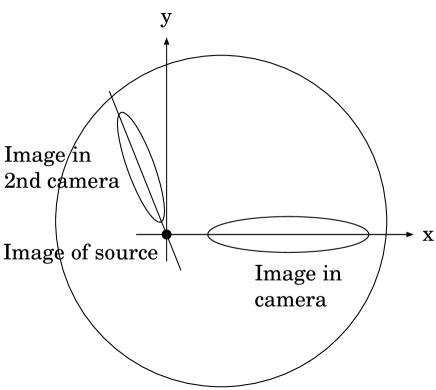
Figure 6: Definition of coordinate systems.

The amplitude $A$ and the timing $t$ of a given pixel will depend on the location $(x,y)$ of the pixel within the image, i.e. on the direction of the photons relative to the shower axis, and on the energy and the impact parameter of an air shower. Here, we are mainly concerned with the timing characteristics; the variation of image amplitudes with energy and core distance is discussed elsewhere in detail [13]. The mean photon arrival time at a pixel at a given $(x,y)$ will primarily vary with the direction under which showers are viewed, i.e., with the core distance $r$. Variations in shower energy, or image size will mainly influence the pixel amplitude, rather than its timing. Therefore, timing characteristics were studied as a function of the pixel location $(x,y)$ and of the reconstructed core distance $r$, averaging over a range of image sizes between 100 and 400 photoelectrons. It was, however, verified that the results given in the following do not significantly depend on the choice of the size band.

Fig. 7 illustrates the amplitude profiles $A(x,y)$ and the time profiles $t(x,y)$ of Cherenkov images for a reconstructed core distance between 100 and 120 m, averaged over many events.

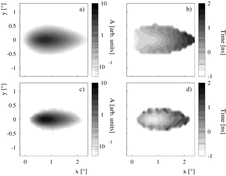
Figure 7: Amplitude profiles using logarithmic scale (a),(c) and time profiles (b),(d) of hadronic showers (a),(b), and of $\gamma$-ray showers (c),(d), for reconstructed core distances $r$ between 100 and 120 m. The profiles were obtained by averaging over many showers, after transforming the images into a common coordinate system.

The amplitude profiles $A(x,y)$ show the familiar features; the images are basically elliptical, but not quite symmetrical in $x$ with respect to the center of gravity of the images. The $\gamma$-ray images are more compact than the images of cosmic-ray showers. The dominant feature of the time profiles $t(x,y)$ of hadronic showers is a gradient along $x$, with a variation of about 3 ns along the image. The effect seems less pronounced for $\gamma$-ray showers. Considering the (modest) $y$-dependence of the time profiles for fixed $x$, one notes that photons on the image axis ($|y|=0$) arrive earliest.

Before going into a more detailed discussion of the data, it may be worth while to illustrate the key dependences of image time profiles using an extremely simplified model (Fig. 8).

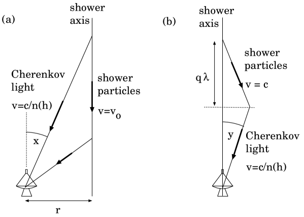
Figure 8: Illustration of the simple model used to estimate time profiles (a) longitudinal (along $x$) and (b) transverse (along $y$).

To describe the dominant longitudinal ($x$) dependence of the timing profile, it is assumed that shower particles propagate along the shower axis until they reach a height $h=r/x$ where the Cherenkov light under consideration is emitted (Fig. 8). The light then propagates to the telescope, taking into account the variation in refractive index. Fig. 9(a) shows the resulting longitudinal profiles under the approximation that shower particles propagate at the speed of light, as justified for electromagnetic showers. Basically, one finds a gradient across the image, which increases with increasing core distance $r$. For small $x$, the curves turn over. At intermediate core distances, photons both from very large height and from very small height tend to arrive late. For large height (small $x$), light propagates over long distances at a speed $c/n$, which is slightly less than the speed of the (particle) shower front. These photons lag behind the shower front. For small height, the additional path length from the shower axis to the telescope causes the delay. The picture changes once a slower speed of propagation for the (particle) shower front is assumed, reflecting, e.g., the fact that hadronic showers are composed of electromagnetic subshowers, continuously fed by a nucleonic or mesonic core cascade. For the TeV showers discussed here, characteristic momenta in this hadronic core of the cascade will be in the range of a few 10 GeV to 100 GeV. For such momenta, the propagation of the shower front is no longer faster than the speed of light in the medium, and light emitted high up in the shower (corresponding to small $x$) arrives first (Fig. 9(b)).

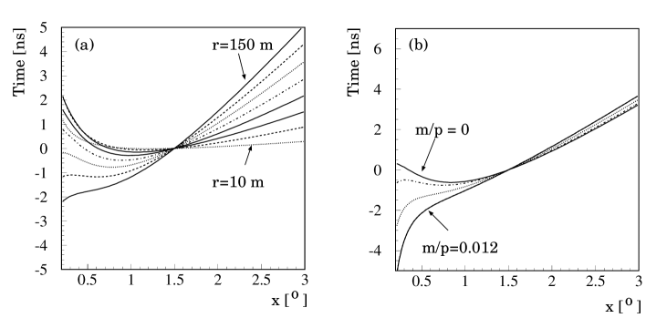
Figure 9: (a) Longitudinal time profile predicted by the simple model, for different core distances $r$ = 10, 30, 50 … 150 m, assuming that the shower propagates at the speed of light. Positive times imply that the light arrives late. For each core distance, the origin $t=0$ is arbitrarily defined as the arrival time for $x=1.5^{\circ}$. (b) Influence of the speed of propagation of the shower front, $v/c=\sqrt{p^{2}/(p^{2}+m^{2})}$, for $m/p$ = 0, 0.005, 0.009, and 0.012, at a fixed core distance of 100 m.

As far as the $y$-dependence is concerned, one can obviously no longer neglect the transverse structure of the air showers. Assuming for simplicity (Fig. 8(b)) that the shower particles generating light at a height $h$ and a distance $d\approx yh$ from the shower axis have their origin on the shower axis at a location $q$ radiation lengths $\lambda$ above the point of emission, and calculating the $y$-dependence of the total path length for both the particles and the light, one finds for the transverse profile

$$t(y)\approx t_{0}+{h\over 2c}\left(1+{h\over q\lambda}\right)y^{2}\\ \approx t_{0}+\left(2.7+{18\over q}\right)y^{2}\mbox{[ns,degr]}~{}~{}~{}.$$

For the numerical values, the typical height of the shower maximum above the HEGRA telescopes, $h\approx 6000$ m, is used. The transverse time profile is parabolic, with a variation of typically 1 ns (using $q\approx 2...3$) across the characteristic transverse spread of $0.3^{\circ}$ of an image.

Figure 10: Longitudinal time profiles $t(x,0)$ of cosmic-ray images, for different ranges in core distance (filled points). The profiles correspond to a slice along $x$ through the image, with $|y|<0.1^{\circ}$. Positive times correspond to late arrival of the photons. Also shown are the corresponding intensity profiles. The smooth lines refer to the simple model for time profiles, using $v/c=\sqrt{p^{2}/(p^{2}+m^{2})}$, with $m/p=0.01$ (lower curve, for small x) and $m/p=0.0033$ (upper curve) for the shower particles.

Fig. 10 shows cuts along $x$ through the time profiles, for small $|y|<0.1^{\circ}$, for cosmic-ray showers with different ranges in core distance. These profiles were obtained by sorting image pixels with $|y|<0.1^{\circ}$ into bins in $x$ according to the coordinates of the pixel centers, and averaging the arrival times in each bin over large samples of showers. For reference, also the intensity profiles are included, defined via the mean amplitude of pixels at a given $x$. In order to avoid a bias in the determination of amplitudes and arrival times, only those images were used which were well contained within the camera. The relatively small bins in $x$ used in Fig. 10 should not hide the fact that the measured profiles correspond to the genuine profile of the Cherenkov light, convoluted with the $0.25^{\circ}$ pixel size. Structures significantly smaller than the pixel size cannot be resolved. Possible systematic effects related to the limited field of view can be checked by noting that time profiles should only depend on the distance $r$ from the telescope to the shower core, but not on the orientation of the shower axis relative to the telescope axis (since the arrival time of photons at the telescope location does not depend on the pointing of the telescope). Indeed, the measured profiles are consistent for shower angles up to $2^{\circ}$ from the telescope axis.

The longitudinal amplitude profiles illustrate the well-known longitudinal asymmetry in the images, the shift of the image centroid with increasing distance to the shower core, and also the increasing length.

For these cosmic-ray showers, one finds – for a given range in core distances – an approximately constant time gradient across the images. The gradient varies almost linearly with distance (Fig. 11), except for small core distances. For medium core distances, around 100 m to 150 m, the simple model reproduces reasonably well the characteristic features of the time profiles. The deviations observed for small core distances and small $x$ are not too surprising, since in this domain the transverse size of the air showers starts to play a role, and $x$ can no longer be regarded as a good measure for the height of photon emission.

Figure 11: Longitudinal time gradient of cosmic-ray images, as a function of core distance. The gradient is determined by fitting a straight line to the data points shown in Fig. 10.

Fig. 12 shows the corresponding time profiles for $\gamma$-ray showers. Overall, time profiles are similar to the ones measured for cosmic-ray showers, with a gradient which becomes increasingly positive for larger core distances. The $\gamma$-ray profiles differ, however, in some details. In particular, the profiles in the 60 m to 120 m distance range show a parabolic rather than linear shape, with photons both from the head and the tail end of the shower arriving late. This difference between $\gamma$-ray showers and cosmic-ray showers at small $x$ is expected, and reflects the difference in the mass of the shower constituents, see Fig. 9(b). Except for small core distances, the simple model with $v=c$ for shower particles does indeed provide a fairly reasonable description of the measured profiles.

Figure 12: Longitudinal time profiles $t(x,0)$ of $\gamma$-ray images, for different ranges in core distance (filled points). The profiles correspond to a slice along $x$ through the image, with $|y|<0.1^{\circ}$. Also shown are the corresponding intensity profiles. The smooth lines refer to the simple model for time profiles, using $v=c$ for the shower particles.

The significant time gradient across the images has consequences for the signal acquisition in Cherenkov telescopes. In many approaches, a gated charge integrator is used to capture pixel signals; to reduce night-sky background, short integration times of order 10 ns to 20 ns are typically used. A fixed and very short signal integration time may result in an underestimate of pixel amplitudes at the head and tail end of the image, in a lower overall image size, and a reduced length of the image. For the current parameters of the HEGRA telescopes, with a signal integration time of two time samples or 17 ns after deconvolution, the differences in image size are small, comparing the amplitudes $A_{o}$ for a fixed integration interval, and the amplitudes $A_{t}$ with a variable interval. For core distances below 100 m, the two image size values differ by less than 2%; the difference rises to about 5% at 200 m and 10% at 300 m. For telescopes with larger mirror areas than the HEGRA telescopes, minimal signal integration times become increasingly important to reduce the noise of the night-sky background light. From our measurements it is, however, clear that signal integration times in the 5 to 10 ns regime are difficult to realize with a common gate applied to all pixels; instead, one needs either very fast transient recording, or an integration gate which is adapted to the individual signals.

For many applications, not only the time profile of images is of interest, but also the fluctuations around the average profile, which are illustrated in Fig. 13. For the selected class of images, with size values between 100 and 400 photoelectrons, the pixel times fluctuate by 1 ns to 2 ns, depending on the location of a pixel. The observed fluctuations are about 50% larger that expected on the basis of the experimental resolution alone, indicating that experimental resolution and shower fluctuations contribute about equally. Fluctuations seem to be slightly smaller for $\gamma$-ray showers as compared to cosmic-ray showers. One notes that for the typical distance range of 100 m to 120 m shown in the figure, the scale of fluctuations is comparable to the time gradient across the image, and to the differences between the two shower types.

Figure 13: Longitudinal time profiles $t(x,\approx 0)$ of cosmic-ray images (a) and of $\gamma$-ray images (b) (filled circles), together with the corresponding amplitude profiles, for a core distance of 100 m to 120 m. The error bars indicate the rms width of the distributions of pixel times at each point along the profile.

Fig. 14 displays transverse profiles, again combining data on timing and amplitudes, both for cosmic-ray showers and $\gamma$-rays. The profiles represent a cut along $y$ at the $x$-value of the peak intensity in the image. The width in particular of the amplitude profiles is of course strongly influenced by the pixel size of $0.25^{\circ}$. Close to the image axis, the time profiles show the expected parabolic shape, $t=t_{0}+\beta y^{2}$, with coefficients $\beta=6$ ns/degr² for cosmic-ray showers and $\beta=12$ ns/degr² for $\gamma$-ray showers, consistent with the model prediction of the order of 10 ns/degr².

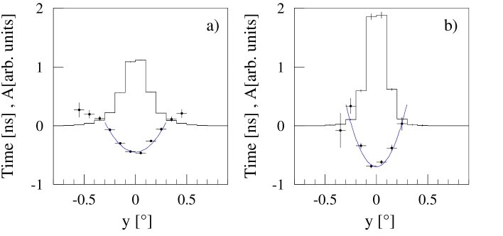
Figure 14: Transverse time profiles $t(x_{max},y)$ of cosmic-ray images (a) and $\gamma$-ray images (b), for core distances between 100 and 120 m (filled points). Also shown are the corresponding intensity profiles. The smooth lines refer to the simple model for time profiles, which predicts a parabolic profile.

6 Applications, including $\gamma$-hadron separation

In the HEGRA IACT system, the use of Flash-ADCs for signal recording was primarily driven by the need to store the signal history for the about 2 $\mu$s required to generate a trigger based on an inter-telescope coincidence, and to propagate the trigger signal back to the telescope; the availability of information on the pixel timing and pulse shapes was only a secondary consideration. Nevertheless, having all this information available, the obvious question is what additional use one can derive from it.

Applications can generally be divided into three classes:

• Improvements in the determination of geometrical shower parameters such as the shower direction, the core location, or possibly the height of the shower maximum. To aid in the determination of shower geometry, one can use the mean arrival time of each image in the different telescopes, and determine a shower direction from the differences in arrival times. Alternatively, one could use the time gradient across the profile to estimate the core distance.

• Improvements in the rejection of cosmic-ray showers. An additional rejection of cosmic-ray showers might by achieved either by exploiting the differences in the time profiles between cosmic-ray showers and $\gamma$-rays, or on the basis of differences in the fluctuations of photon arrival times.

• Consistency checks concerning the interpretation of shower images. Rather than trying to improve the reconstruction or identification of shower events, the timing information could be used to provide on a statistical basis an independent confirmation, e.g. of the $\gamma$-ray nature of a given sample of showers.

Here, two selected issues will be addressed, namely the use of the time gradient over the image for the shower reconstruction, and the hadron rejection based on the time structure of images. The use of the average event timing for the reconstruction of the shower direction was discussed in [15].

The time gradient along the major axis of Cherenkov images can be used to determine where the head and tail ends of the image are, at least if the core distance is approximately known. To study how reliable such a technique is, a linear time gradient was fitted to the individual images, taking into account the estimated errors for the timing values of the individual pixels. Fig. 15 illustrates what fraction of the $\gamma$-ray images have a positive gradient, i.e. d$t$/d$x>0$, as a function of the core distance. As already evident from Fig. 12, events with small core distances tend to have negative slopes, events with large distances have positive slopes. For distances less than about 60 m and for distances greater than 100 m, the orientation of the image can be determined with 75% reliability. For stereoscopic systems, this information is of course of limited use, since the stereoscopic reconstruction will anyway resolve the usual head-tail ambiguities.

Figure 15: Fraction of $\gamma$-ray events with a positive time gradient along $x$, as a function of the core distance.

Information concerning the orientation of images is much more relevant for single Cherenkov telecopes. Based on the results shown in Fig. 15, it is however nontrivial to make statements about the performance in the single telescope case, because there the information on impact distance is poorer and also the distribution of impact distances will be different than for the IACT system.

Image timing information has been repeatedly proposed for use in $\gamma$-hadron discrimination. Hadron images should show a larger timing spread [7], and in particular ”precursor” signals at early times caused by Cherenkov light emitted from high-energy muons [7, 14].

There are two different approaches to using the timing information: one option is to use the full signal waveform, as recorded by the Flash-ADC system, before or after deconvolution. In this case, one would typically sum over the waveform for all image pixels, and then calculate the width of the pulse or look for precursors or a tail in the waveform. One could also consider the pulse widths measured for the individual pixels. An alternative is to use the timing values derived for each pixel, and to calculate the width of the distribution, or look for early or late pixels. With a sampling rate of the Flash-ADCs of 120 MHz, one is obviously not very sensitive to differences in pulse shapes at the level of at most a few ns, as they are expected between $\gamma$-ray images and cosmic-ray images. Work therefore concentrated on the spread of the light arrival times measured in the different pixels of an image; here, the experimental resolution is in the relevant (ns) range.

Several different approaches were tried. For example, Fig. 16(a) shows the rms spread of pixel times with respect to the time profile expected for $\gamma$-ray images. One rms value is calculated using all pixels of a given image, and the distribution of this rms spread is plotted for $\gamma$-ray images and for cosmic-ray background events. Cosmic-ray events clearly show a larger spread among pixel times, compared to $\gamma$-ray images. However, the differences are not significant enough to allow an efficient separation; at most, a Q-factor of around 1.1 is reached.

Figure 16: Distribution of the rms spread per image of pixel times, relative to the nominal time profile expected for $\gamma$-ray events. Open symbols indicate cosmic-ray events, closed symbols $\gamma$-ray images. (a) For all events, (b) after selecting $\gamma$-ray candidates on the basis on image shape.

In addition, the timing information is highly correlated with the image shapes. Once $\gamma$-ray candidates are selected on the basis of cuts on the mean scaled width of all images, the time spread among image pixels is almost identical for $\gamma$-ray images and for cosmic rays (Fig. 16(b)).

Various other techniques to use the timing information for discrimination were investigated, with similar results; in no case a reasonably clear-cut difference between $\gamma$-ray images and cosmic rays was seen. These results differ from the conclusions obtained in [7], where an improvement of significance with an analysis of signal shapes was obtained even after shape cuts. However, the hardware setups and analysis techniques differ significantly. Also, the trigger conditions and shape cuts used in case of the HEGRA stereoscopic system provide a much stronger pre-selection than in case of the single telescope of  [7].

7 Summary

Using air showers observed with the stereoscopic HEGRA IACT system, with their precisely reconstructed direction and core location, the mean arrival time of Cherenkov photons was studied as a function of the direction of these photons, i.e., of their location within the shower image, and as a function of the core distance. The key feature of cosmic-ray induced images is a roughly linear variation of arrival times along the major axis of an image. The gradient varies almost linearly with the core distance, from values of about -1 ns/^∘ for small distances to more than 5 ns/^∘ for large distances. In the transverse direction, along the minor axis, a parabolic profile is observed, with photons on the major axis of the image arriving earliest. Gamma-ray images differ from cosmic-ray images in that particles at small angles – emitted at large height – tend to arrive later than the bulk of the image photons. Only at larger core distances, well beyond 100 m, does the linear variation along the major axis become the main feature.

These features of the time profiles of Cherenkov images can be explained in a semi-quantitative fashion as an interplay between the speed of propagation of the shower front, and the speed of propagation of Cherenkov photons on their way from the point of emission to the telescope.

The observed variation of photon arrival times imposes a lower limit on the signal integration time used in Cherenkov telescopes; if a common integration gate is used for all pixels, gate times significantly below 10 ns will result in a distortion of image parameters, and possibly in a reduced gamma-hadron separation.

The use of pixel timing to achieve improved $\gamma$-hadron separation and towards resolving the head-tail ambiguity of the images is discussed. Concerning $\gamma$-hadron separation, one finds that timing information is not a very efficient method of hadron rejection. The timing information is strongly correlated with the information contained in images’ shapes; after an efficient selection on the basis of shapes, no further improvement was possible. Timing can be used to resolve head-tail ambiguities to a certain extent. In the case of the HEGRA IACT system, the timing information provided by the 120 MHz Flash-ADC system is valuable for consistency checks and for the fine-tuning of the simulation, but does not significantly improve the performance of the system. We believe that even with waveform recording at higher frequencies, the gain is quite limited in the case of IACT systems, since trigger conditions and shape cuts preselect a ‘$\gamma$-ray like’ sample of hadronic showers, which also in their timing properties behave much like $\gamma$-induced showers. The situation may be different for single IACTs, with their less stringent preselection, see e.g. [7].

References

- [1] see, e.g., T.C. Weekes, Space Science Rev. 75 (1996) 1; M. F. Cawley and T.C. Weekes, Experimental Astronomy 6 (1996) 7.
- [2] A. Daum et al., Astroparticle Phys. 8 (1997) 1.
- [3] F. Aharonian et al., Astron. Astrophys. 327 (1997) L5.
- [4] For an overview, see e.g. R.J. Protheroe et al., Proc. of the 25 Int. Cosmic Ray Conf., Durban, Vol. 8, p. 317 (1997), and astro-ph 9710118.
- [5] M. Heß, Ph.D. Thesis, Heidelberg 1998.
- [6] J.R. Patterson and A.M. Hillas, J. Phys. G 9 (1983) 323.
- [7] M.D. Roberts et al., J. Phys. G 24 (1998) 255.
- [8] C. Köhler et al., Astropart. Phys. 6 (1996) 343.
- [9] N. Bulian et al., Astropart. Phys. 8 (1998) 223.
- [10] A.M. Hillas, Proc. 19th ICRC (La Jolla, 1985) Vol. 3, 445.
- [11] M. Heß, Diploma Thesis, Heidelberg, 1995.
- [12] M. Hemberger, Ph.D. Thesis, Heidelberg, 1998.
- [13] F. Aharonian et al., Astropart. Phys., in press, and astro-ph/9807119.
- [14] H. Cabot et al., astro-ph/9708236 (1997).
- [15] M. Heß, Proc. 25th ICRC (Durban, 1997), Vol. 5,133.