Cosmological Tracking Solutions

Abstract

A substantial fraction of the energy density of the universe may consist of quintessence in the form of a slowly-rolling scalar field. Since the energy density of the scalar field generally decreases more slowly than the matter energy density, it appears that the ratio of the two densities must be set to a special, infinitesimal value in the early universe in order to have the two densities nearly coincide today. Recently, we introduced the notion of tracker fields to avoid this initial conditions problem. In the paper, we address the following questions: What is the general condition to have tracker fields? What is the relation between the matter energy density and the equation-of-state of the universe imposed by tracker solutions? And, can tracker solutions explain why quintessence is becoming important today rather than during the early universe?

I Introduction

Quintessence[1] has been proposed as the missing energy component that must be added to the baryonic and matter density in order to reach the critical density.[2, 3] Quintessence is a dynamical, slowly-evolving, spatially inhomogeneous component with negative pressure. An example is a scalar field $Q$ slowly rolling down its potential $V(Q)$.[1, 4, 5, 6, 7, 8, 9, 10, 11] For a general scalar field, the pressure is $p_{Q}=\frac{1}{2}\dot{Q}^{2}-V$, and the energy density is $\rho_{Q}=\frac{1}{2}\dot{Q}^{2}+V$. For a slowly rolling scalar field, the pressure can be negative if the kinetic energy is less than the potential energy. For quintessence, the equation-of-state, defined as $w_{Q}=p_{Q}/\rho_{Q}$, lies between 0 and $-1$. Depending on $V(Q)$, $w_{Q}$ may be constant, slowly-varying, rapidly varying or oscillatory.[1]

A key problem with the quintessence proposal is explaining why $\rho_{Q}$ and the matter energy density should be comparable today. There are two aspects to this problem. First of all, throughout the history of the universe, the two densities decrease at different rates, so it appears that the conditions in the early universe have to be set very carefully in order for the energy densities to be comparable today. We refer to this issue of initial conditions as the “coincidence problem.”[12] This is a generalization of the flatness problem described by Dicke and Peebles in 1979;[13] the very same issue arises with a cosmological constant as well. A second aspect, which we call the “fine-tuning problem,” is that the value of the quintessence energy density (or vacuum energy or curvature) is very tiny compared to typical particle physics scales. The fine-tuning condition is forced by direct measurements; however, the initial conditions or coincidence problem depends on the theoretical candidate for the missing energy.

Recently, we introduced a form of quintessence called “tracker fields” which avoids the coincidence problem.[14] Tracker fields have an equation-of-motion with attractor-like solutions in which a very wide range of initial conditions rapidly converge to a common, cosmic evolutionary track. The initial value of $\rho_{Q}$ can vary by nearly 100 orders of magnitude without altering the cosmic history. The acceptable initial conditions include the natural possibility of equipartition after inflation – nearly equal energy density in $Q$ as in the other 100-1000 degrees of freedom (e.g., $\Omega_{Qi}\approx 10^{-3}$). Furthermore, the resulting cosmology has desirable properties. The equation-of-state $w_{Q}$ varies according to the background equation-of-state $w_{B}$. When the universe is radiation-dominated ($w_{B}=1/3$), then $w_{Q}$ is less than or equal to 1/3 and $\rho_{Q}$ decreases less rapidly than the radiation density. When the universe is matter-dominated ($w_{B}=0$), then $w_{Q}$ is less than zero and $\rho_{Q}$ decreases less rapidly than the matter density. Eventually, $\rho_{Q}$ surpasses the matter density and becomes the dominant component. At this point, $Q$ slows to a crawl and $w_{Q}\rightarrow-1$ as $\Omega_{Q}\rightarrow 1$ and the universe is driven into an accelerating phase. These properties seem to match current observations well.[15]

In some cases, $w_{Q}$ is very nearly equal to $w_{B}$ during the radiation- and matter-dominated epochs, and some authors have focused on the fact that the $Q$ energy density decreases at nearly the same rate as the background energy density.[10, 16] However, our focus is on the fact that the cosmology is independent of initial conditions, which includes but does not require $w_{Q}\approx w_{B}$ during the matter- and radiation-dominated epochs. Hence, our use of the term “tracker” is meant to refer to solutions joining a common evolutionary track, as opposed to tracking closely the background energy density.

It is also an interesting point that some tracker solutions do not require small mass parameters to obtain a small energy density today;[14, 17] whether this is a satisfactory solution to the fine tuning problem is debatable, though. We do not explore this issue in this paper.

The tracker solution differs from a classical dynamics attractor because it is time-dependent: during tracking, $\Omega_{Q}$ increases steadily. This contrasts with the solutions based on exponential potentials recently discussed by Ferreira and Joyce[10] in which $\Omega_{Q}$ is constant during the matter dominated epoch. For this kind of solution, $\Omega_{Q}$ is constrained to be small ($\Omega_{Q}\leq 0.15$) at the beginning of matter domination in order that large-scale structure be formed, but then it cannot change thereafter. Hence, it remains a small, subdominant component. (See, however, discussion of undershoot and overshoot solutions later in this paper for a possible way around this constraint.) The tracker solution is more desirable, though, because it enables the $Q$-energy to eventually overtake the matter density and induce a period of accelerated expansion, which produces a cosmology more consistent with measurements of the matter density, large scale structure, and supernovae observations.[15, 18]

An important consequence of the tracker solutions is the prediction of a relation between $w_{Q}$ and $\Omega_{Q}$ today.[14] Because tracker solutions are insensitive to initial conditions, both $w_{Q}$ and $\Omega_{Q}$ only depend on $V(Q)$. Hence, for any given $V(Q)$, once $\Omega_{Q}$ is measured, $w_{Q}$ is determined. In general, the closer that $\Omega_{Q}$ is to unity, the closer $w_{Q}$ is to $-1$. However, since $\Omega_{m}\geq 0.2$ today, there is a sufficient gap between $\Omega_{Q}$ and unity that $w_{Q}$ cannot be so close to $-1$. We find that $w_{Q}\gtrsim-0.8$ for practical models. This $w_{Q}$-$\Omega_{Q}$ relation, which makes the tracker field proposal distinguishable from the cosmological constant, will be explored further in this paper.

The purpose of the present paper is to expand on our introductory article on tracker fields and the coincidence problem. In particular, we want to go beyond the specific examples of tracker potentials studied before and address in a general way the following questions (the relevant section is shown in parentheses):

• What is a tracker solution? (II.B)

• What potentials $V(Q)$ have tracker solutions and which do not? (III.A-C,F)

• How does convergence of diverse initial conditions to a common track occur? (III.D)

• What additional conditions on tracking potentials are required to make them useful and practical? (III.H)

• How does tracking result in the prediction of an $\Omega_{Q}$-$w_{Q}$ relation? (IV)

• What range of $w_{Q}$ today is possible for tracking solutions according to the $w_{Q}$-$\Omega_{Q}$ relation? (IV)

• Why is the $Q$-field first beginning to dominate at this late stage of the universe rather than at some early stage? (V)

II Definitions and Basic Equations

We shall consider a scalar field with present equation-of-state $-1<w_{Q}<0$ in a flat cosmological background (consistent with inflation). The ratio of the energy density to the critical density today is $\Omega_{Q}$ for the $Q$-field and $\Omega_{m}$ for the baryonic and dark matter density where $\Omega_{m}+\Omega_{Q}=1$. We use dimensionless units where the Planck mass is $M_{p}=1$.

A The Tracker Equation

The equation-of-motion for the $Q$-field is

$$\ddot{Q}+3H\dot{Q}+V^{\prime}=0$$ (1)

where

$$H^{2}=\left(\frac{\dot{a}}{a}\right)^{2}=\kappa(\rho_{m}+\rho_{r}+\frac{1}{2}\dot{Q}^{2}+V)$$ (2)

where $a$ is the Robertson-Walker scale factor, $\rho_{m}$ is the matter density, $\rho_{r}$ is the radiation energy density, and $\kappa=\frac{8\pi}{3}$. The definition of the equation-of-state is

$$w_{Q}=\frac{p}{\rho}=\frac{\frac{1}{2}\dot{Q}^{2}-V}{\frac{1}{2}\dot{Q}^{2}+V}.$$ (3)

It is extremely useful to combine these relations into an unfamiliar form, which is the form we would like the reader to have in mind when we refer to the “equation-of-motion”:

$$\pm\frac{V^{\prime}}{V}=3\sqrt{\frac{\kappa}{\Omega_{Q}}}\sqrt{1+w_{Q}}\left[1+\frac{1}{6}\frac{d\,\ln{x}}{d\,\ln{a}}\right]$$ (4)

where $x=(1+w_{Q})/(1-w_{Q})=\frac{1}{2}\dot{Q}^{2}/V$ is the ratio of the kinetic to potential energy density for $Q$ and prime means derivative with respect to $Q$. The $\pm$ sign depends on whether $V^{\prime}>0$ or $V^{\prime}<0$, respectively. The tracking solution (to which general solutions converge) has the property that $w_{Q}$ is nearly constant and lies between $w_{B}$ and $-1$. For $1+w_{Q}={\cal O}(1)$, $\dot{Q}^{2}\approx\Omega_{Q}H^{2}$ and the equation-of-motion, Eq. (4), dictates that

$$\frac{V^{\prime}}{V}\approx\frac{1}{\sqrt{\Omega_{Q}}}\approx\frac{H}{\dot{Q}}$$ (5)

for a tracking solution; we shall refer to this as the “tracker condition.”

An important function is $\Gamma\equiv V^{\prime\prime}V/(V^{\prime})^{2}$, whose properties determine whether tracking solutions exist. Taking the derivative of the equation-of-motion with respect to $Q$ and combining with the equation-of-motion itself, we obtain the equation:

$$\Gamma\equiv\frac{V^{\prime\prime}V}{(V^{\prime})^{2}}=1+\frac{w_{B}-w_{Q}}{2(1+w_{Q})}-\frac{1+w_{B}-2w_{Q}}{2(1+w_{Q})}\frac{\dot{x}}{6+\dot{x}}$$ (6)

$$-\frac{2}{(1+w_{Q})}\frac{\ddot{x}}{(6+\dot{x})^{2}}$$ (7)

where $\dot{x}\equiv d\,\ln{x}/d\,\ln{a}$ and $\ddot{x}\equiv d^{2}\,\ln{x}/d\,\ln{a}^{2}$. We will refer to this equation as the “tracker equation.”

B What is a tracker solution?

We shall use the term “converging” to refer to the attractor-like behavior in which solutions to the equation-of-motion are drawn towards a common solution, $\tilde{Q}(t)$. We shall argue that converging solutions with $w_{Q}\leq w_{B}$ solve the coincidence problem. A tracker solution is one which undergoes long periods of converging. The converging period should be long enough so that any residue of initial condition is washed away and the solution today only depends on parameters in the potential. For a potential $V(Q)=M^{4}\tilde{v}(Q/M)$ (where $\tilde{v}$ is a dimensionless function of $Q/M$), there is a family of tracker solutions parameterized by $M$. The value of $M$ is determined by the measured value of $\Omega_{m}$ today (assuming a flat universe).

We make the (fine) distinction between “tracking” and “converging” because tracker solutions typically go through some periods when solutions are not approaching one another. In particular, during transitions in the background equation-of-state, such as the transition from radiation- to matter-domination, there are brief intervals during which $w_{Q}$ changes rapidly and general solutions are not drawn towards the tracker solution; fortunately, these transitory periods are too short to spoil the advantages of tracking solutions.

To be complete in classifying the possibilities, one should also consider potentials in which $Q$ first passes through a regime where solutions converge and then ends up in a regime where they do not. We refer to these as “hybrid models” below. By the time the second regime is reached, sufficient convergence of solutions may have already occurred to insure that the desired range of initial conditions track along a common solution in the second regime.

III Properties of Tracking Solutions and Tracking Potentials

In the following section, we prove the key properties of tracker solutions. Each subsection leads with a summary statement of the result for those who wish to skip the detailed mathematical arguments.

A What potentials have converging behavior and tracker solutions and which do not?

Our central theorem is that tracking behavior with $w_{Q}<w_{B}$ occurs for any potential in which $\Gamma\equiv V^{\prime\prime}V/(V^{\prime})^{2}>1$ and is nearly constant ($|d(\Gamma-1)/Hdt|\ll|\Gamma-1|$) over the range of plausible initial $Q$. For the cases of interest, the range extends to $V(Q)$ equal to the initial background energy density $\rho_{B}$ down to $V(Q)$ equal to the background density at matter-radiation equality, a span of over 100 orders of magnitude. Although $w_{Q}<w_{B}$ is what is desired for most practical applications, we also show that tracking behavior with $w_{B}<w_{Q}<(1/2)(1+w_{B})$ is possible provided $1-(1-w_{B})/(6+2w_{B})<\Gamma<1$ and nearly constant. Tracking does not occur for $\Gamma<1-(1-w_{B})/(6+2w_{B})$.

Hence, testing for the existence of tracking solutions reduces to a simple condition on $V(Q)$ without having to solve the equation-of-motion directly. In particular, the condition that $\Gamma\approx\,{\rm constant}$ can be evaluated either by testing

$$\left|\Gamma^{-1}\frac{d(\Gamma-1)}{Hdt}\right|\approx\left|\frac{\Gamma^{\prime}}{\Gamma\,(V^{\prime}/V)}\right|\ll 1$$ (8)

over range of $Q$ corresponding to the allowed initial conditions; the middle expression is easily computed knowing $V(Q)$ only without having to solve an equation-of-motion. (Here we have used the tracker condition $\dot{Q}/H\approx\sqrt{\Omega_{Q}}\approx V^{\prime}/V$ which applies for the tracker solution.) An equivalent condition is that that $\Delta\Gamma/\Gamma\ll 1$,  where $\Delta\Gamma$ is the difference between the maximum and minimum values of $\Gamma$ over the same range of $Q$. The condition $\Gamma>1$ is equivalent to the constraint that $|V^{\prime}/V|$ be decreasing as $V$ decreases. These conditions encompass an extremely broad range of potentials, including inverse power-law potentials ($V(Q)=M^{4+\alpha}/Q^{\alpha}$ for $\alpha>0$) and combinations of inverse power-law terms (e.g., $V(Q)=M^{4}{\rm exp}(M/Q)$). Some potentials of this form are suggested by particle physics models with dynamical symmetry breaking or nonperturbative effects.[17, 19, 20, 21, 22, 23, 24]

If $w_{Q}<w_{B}$, converging behavior does not occur for potentials in which $|V^{\prime}/V|$ strictly increases as $V$ decreases ($\Gamma<1$). This category includes quadratic potentials and most examples of quintessence models in the literature. Instead of converging behavior, these models require specially tuned initial conditions to obtain an acceptable value of $\Omega_{Q}$ today, as discussed in Section III.B.

For $(1/2)(1+w_{B})>w_{Q}>w_{B}$, converging behavior does occur if $V^{\prime}/V$ is strictly increasing as $V$ decreases ($\Gamma<1$); however, as we explain in Section III.F, potentials with $w_{Q}>w_{B}$ do not produce viable cosmological models: if $w_{Q}>w_{B}$ and $\Omega_{Q}\geq 1/2$ today (as suggested by current observation) then $\Omega_{Q}$ must exceed $\Omega_{m}$ in the past and there is no period of matter-domination or structure formation.

Hybrid potentials are possible in which converging behavior only occurs for a finite period during the early universe, provided that the time is sufficiently long to bring together solutions whose initial conditions span the range of practical interest. For example, one can construct potentials in which $|V^{\prime}/V|$ decreases at first as $Q$ rolls downhill, and then $|V^{\prime}/V|$ begins to increase. Another possibility is that $|V^{\prime}/V|$ increases at first and $w_{Q}>w_{B}$, as discussed in the previous paragraph. We pointed out that this condition allows convergence, but cannot be maintained up to the present for practical reasons of structure formation. However, the condition could be maintained for a long, finite period in the early universe so long as it is terminated before matter-domination.

B Why do models with increasing $|V^{\prime}/V|$ and $w_{Q}<w_{B}$ fail to solve the coincidence problem?

For potentials in which $|V^{\prime}/V|$ increases as $V$ decreases ($\Gamma<1$), the LHS of the the equation-of-motion Eq. (4) is increasing. If $w_{Q}<w_{B}$, $1/\sqrt{\Omega_{Q}}$ on the RHS is decreasing as $Q$ rolls downhill. Hence, the tracker condition, $|V^{\prime}/V|\sim 1/\sqrt{\Omega_{Q}}$, cannot be maintained and $w_{Q}$ cannot be maintained at a nearly constant value (different from $-1$) for any extended period.

In particular, extrapolating backwards in time, $|V^{\prime}/V|$ is strictly decreasing and $1/\sqrt{\Omega_{Q}}$ is strictly increasing. The only way to satisfy the equation-of-motion, Eq. (4), is to have $w_{Q}$ approach $-1$. But, this corresponds to the $Q$-field freezing at some value $Q=Q_{i}$ after only a few Hubble times. The energy density of the frozen field is only slightly higher than the current energy density. Consequently, to obtain this cosmological solution, one has to have special initial conditions in the early universe (after inflation, say) that set $Q$ precisely to $Q_{i}$ and the $Q$-energy density to $\rho_{Q_{i}}$, a value nearly 100 orders of magnitude smaller than the background energy density. It is precisely this tuning of initial conditions (the coincidence problem) which we seek to avoid.

We note that many quintessence models ($w_{Q}<0$) discussed in the literature fall into this non-tracking class and require extraordinary tuning of initial conditions. Simple examples include the harmonic potential, $V(Q)=M^{2}Q^{2}$, and the sinusoidal potential, $V(Q)=M^{4}\,[\cos{(Q/f)}+1]$. In these models, the initial value of $Q$ must be set to a specific value initially in order to obtain the measured value of $\Omega_{Q}$ today.

C What determines the tracker solution?

Our claim is that solutions converge to a tracker solution if: (a) $\Gamma(Q)=V^{\prime\prime}V/(V^{\prime})^{2}$ is nearly constant; and (b) $\Gamma>1$ for $w_{Q}<w_{B}$ or $\Gamma<1$ for $(1/2)(1+w_{B})>w_{Q}>w_{B}$. We have explained in the previous section why $\Gamma$ must be greater than unity if $w_{Q}<w_{B}$ or else the tracking condition, $V^{\prime}/V\sim 1/\sqrt{\Omega_{Q}}$, cannot be maintained. A similar argument requires $1-(1-w_{B})/(6+2w_{B})<\Gamma<1$ if $(1/2)(1+w_{B})>w_{Q}>w_{B}$. But, as we shall see, we also need that $\Gamma$ be nearly constant in order to have converging behavior.

If $\Gamma$ is nearly constant, then the tracker equation, Eq. (6), implies that there is a solution in which $w_{Q}$ is nearly constant and $x$ and its time-derivatives are negligible. In this case, we have that the equation-of-state for the $Q$-field is nearly constant:

$$w_{Q}\approx\frac{w_{B}-2(\Gamma-1)}{1+2(\Gamma-1)}.$$ (9)

If $\Gamma>1$, the value of $w_{Q}$ must be less than $w_{B}$ to satisfy the tracker equation, which means that the $Q$-energy red shifts more slowly than the background energy. For inverse power-law potentials $V(Q)=M^{4+\alpha}/Q^{\alpha}$, $\Gamma=1+\alpha^{-1}$, and the relation we have derived matches the relation in our first paper.[14] For $V(Q)=M^{4}{\rm exp}(1/Q)$, $\Gamma=1+2Q$, which satisfies our condition for $Q\ll 1$. For $\Gamma<1$, the same relation says that the value of $w_{Q}$ must be greater than $w_{B}$; but we also require that $\Gamma>1-(1-w_{B})/(6+2w_{B})$ in order to satisfy the criterion, $w_{Q}<(1/2)(1+w_{B})$, necessary to have converging solutions (see Section III.F).

If $\Gamma$ varies significantly with $Q$, then one can find a wide and continuous distribution of $Q$, $\Omega_{Q}$, and $w_{Q}$ which satisfies the tracker equation. Hence, there is no single solution to which solutions converge.

In sum, we have succeeded in expressing our conditions for tracking solutions in terms of $\Gamma$, which depends entirely on the functional form of $V$. A simple computation of $V^{\prime\prime}V/(V^{\prime})^{2}$ determines if $V$ admits tracking solutions or not. The case of interest for quintessence is $w_{Q}<w_{B}$, in which case the condition for a tracker solution is $\Gamma>1$ and nearly constant.

D How is the tracker solution approached beginning from different initial conditions?

We shall call the tracker solution $\tilde{Q}(t)$ and the energy density of the tracker solution as a function of time $\rho_{\tilde{Q}}(t)$. This subsection explains in rough detail how solutions converge to the tracker solution for any initial $\rho_{Q}$ that lies between the initial background energy density, $\rho_{Bi}$, and the current critical density, $\rho_{c0}$. This range stretches nearly 100 orders of magnitude. In particular, we explain how the convergence to the tracker solution is different if initially $\rho_{B}>\rho_{Q}>\rho_{\tilde{Q}}$ versus $\rho_{c0}<\rho_{Q}<\rho_{\tilde{Q}}$. For simplicity, we confine ourselves to the case $w_{Q}<w_{B}$. We complete the proof of convergence in the next subsection.

The equation-of-motion, Eq. (4) can be rearranged as:

$$\frac{1}{6}\frac{d\,\ln{x}}{d\,\ln{a}}=-\frac{1}{3\sqrt{\kappa(1+w_{Q})}}\sqrt{\Omega_{Q}}\frac{V^{\prime}}{V}-1\equiv\Delta(t)-1;$$ (10)

where we have restricted ourselves for simplicity to potentials with $V^{\prime}<0$. Then, since $V^{\prime}<0$, the RHS of this equation is a balance between a positive semi-definite term ($\Delta$) and a negative term. The tracker condition corresponds to the two conditions: $1-w_{Q}^{2}$ significantly different from zero and $w_{Q}$ nearly constant. The latter requires near balance on the RHS above ($\Delta\approx 1$) so that $d\,\ln{x}/d\,\ln{a}$ is nearly zero.

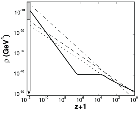
FIG. 1.: Energy density versus red shift for the evolution of a tracker field. For computational convenience, $z=10^{12}$ (rather than inflation) has been arbitrarily chosen as the initial time. The white bar on left represents the range of initial $\rho_{Q}$ what leads to undershoot and the grey bar represents overshoot, combining for a span of more than 100 orders of magnitude if we extrapolate back to inflation. The solid black circle represents the unique initial condition required if the missing energy is vacuum energy density. The solid thick curve represents an “overshoot” in which $\rho_{Q}$ begins from a value greater than the tracker solution value, decreases rapidly and freezes, and eventually joins the tracker solution.

First, consider the “overshoot” case in which $\rho_{Q}$ is initially much greater than the tracker value $\rho_{\tilde{Q}}$. For simplicity, let us assume that $Q$ is released from rest. The evolution goes through four stages, illustrated in Figures 1-3. The potential for this exampleis $V(Q)=M^{4}/Q^{6}$. (For this and all subsequent figures, the choice of $z=10^{12}$ has been chosen as the initial time for convenience of computation and illustration; a realistic figure would have initial $z$ corresponding to the inflationary scale.)

1. $V^{\prime}/V$ and $\Omega_{Q}$ are so big initially that $\Delta\gg 1$. So,

   $$\frac{1}{6}\frac{d\,\ln{x}}{d\,\ln{a}}=\frac{2}{1-w_{Q}^{2}}\frac{d\,\ln{w_{Q}}}{Hdt}\gg 1$$ (11)

   and $w_{Q}$ is driven towards its maximal value, $w_{Q}\rightarrow\,+1$. This means that $\dot{Q}$ becomes large and $V$ decreases very rapidly as $Q$ runs downhill.

2. As $Q$ runs downhill, $V^{\prime}/V$ and $\Omega_{Q}$ are decreasing. Consequently, $\Delta$ begins to decrease and ultimately reaches a value of order unity, one of the requirements for a tracker solution. However, $w_{Q}$ has been driven towards $+1$; up to this point, the RHS of Eq. (10) has been positive, so there has been no opportunity for $w_{Q}$ to decrease. As a result, $1-w_{Q}^{2}$ is too small, or, more specifically, the kinetic energy is too large for $Q$ to join the tracker solution. Hence, $Q$ rolls farther down the potential, overshooting the tracker solution.

3. Once the tracker solution is overshot, $\Delta$ becomes less than unity and the RHS of Eq. (10) changes sign. $w_{Q}$ now decreases from $+1$ towards $-1$. One might wonder what happens when $w_{Q}$ crosses through the tracker value; why doesn’t $Q$ track at this point? The answer is that there is now the problem that $\Delta$ is too small. So, the RHS of Eq. (10) remains too negative and $w_{Q}$ continues to decreases and heads towards $-1$.

4. Once $w_{Q}$ reaches close to $-1$, $Q$ is essentially frozen at some value $Q_{f}$ and, consequently, $V$ and $V^{\prime}/V$ are frozen. However, $\Delta$ is now increasing since $\Omega_{Q}$ is increasing – even though $\rho_{Q}$ is nearly constant, $\rho_{B}$ is decreasing. As $\Delta$ increases to order unity, the sign of Eq. (10) changes once again; $w_{Q}$ increases from $-1$; the field runs downhill; and, the sign of Eq. (10) changes yet again. After a few oscillations, the terms in Eq. (10) settle into near balance and $Q$ is on track.

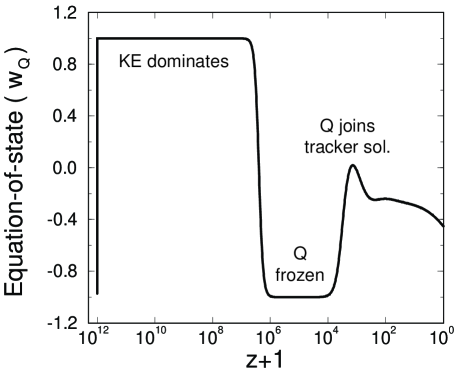
FIG. 2.: A plot of $w_{Q}$ vs. red shift for the overshoot solution shown in Figure 1. $w_{Q}$ rushes immediately towards $+1$ and $Q$ becomes kinetic energy dominated. The field freezes and $w_{Q}$ rushes towards $-1$. Finally, when $Q$ rejoins the tracker solution, $w_{Q}$ increases, briefly oscillates and settles into the tracker value.

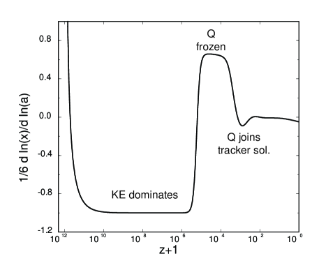
FIG. 3.: A plot of $\dot{x}/6=(1/6)\,d\,\ln{x}/d\,\ln{a}$ for the overshoot solution shown in Figures 1 and 2. At late times when $Q$ settles into the tracker solution, $\dot{x}$ is small and $w_{Q}$ is nearly constant. During the overshoot phase, $\dot{x}$ undergoes large positive and negative changes, as described in the text.

Next, consider the “undershoot” case in which $\rho_{Q}$ is initially much less than the tracker value $\rho_{\tilde{Q}}$ and $Q$ is released from rest. This corresponds to $Q\gg\tilde{Q}$ initially. By assumption, $V$ and $|V^{\prime}/V|$ are much smaller than the tracker value. Consequently, $1/\sqrt{\Omega_{Q}}$ is larger than the tracker value. The only way to satisfy the equation-of-motion, Eq. (4) is for $w_{Q}$ to approach $-1$ so that the coefficient of $1/\sqrt{\Omega_{Q}}$ is nearly zero. This condition corresponds to a very small kinetic energy density or $Q$ nearly constant. Hence, the field remains nearly “frozen”, and $V$ and $V^{\prime}/V$ are nearly constant as the universe evolves. The situation is identically to beginning with Step 4 above, and the scenario proceeds just as described there.

In sum, the field either drops precipitously past the tracker value and is frozen (overshoot), or it begins with a value less than the tracker solution (undershoot) and is frozen. In either case, it proceeds from the frozen state to joining the tracker solution. In the case of undershoot, the frozen value $Q_{f}$ is simply the initial value of $Q$. For the overshoot case, $Q$ begins by going through a kinetic energy dominated period in which $\dot{Q}\propto a^{-3}$. If the initial $\rho_{Qi}<\rho_{Bi}$, where $\rho_{B}$ is the background radiation density, then $a\propto t^{1/2}$ and the frozen value of $Q$ is

$$Q_{f}\approx Q_{i}+\sqrt{\frac{3}{4\pi}\Omega_{Q_{i}}}$$ (12)

where the subscript refers to the initial values of $Q$ and $\Omega_{Q}$. (If initially $\rho_{Qi}>\rho_{Bi}$, then $a\propto t^{1/3}$, and

$$Q_{f}\approx Q_{i}+\sqrt{\frac{3}{4\pi}}(1+\frac{1}{2}\ln{\frac{\rho_{Qi}}{\rho_{B}}});$$ (13)

in this case, $Q_{f}$ is so large that $Q$ remains frozen up to the present time.) For the overshoot case, $Q_{i}$ is typically very small compared to unity and $\Omega_{Qi}={\cal O}(1)$. Consequently, the frozen value $Q_{f}$ depends on $\Omega_{Qi}$ only.

Initial conditions in which $\dot{Q}_{i}$ is non-zero do not change the story significantly. If $\dot{Q}_{i}$ is very large, then the initial behavior is kinetic energy dominated, and the evolution proceeds similar to the overshoot case. Initial fluctuations in $Q$ also do not change the story since they are exponentially suppressed once the potential becomes non-negligible and the field is driven towards the tracker solution (see Appendix).

The possibility of overshoot and undershoot allows a new possibility for the case of exponential potentials recently discussed by Ferreira and Joyce.[10] The exponential potential is a special example of a tracker solution in which $\Omega_{Q}$ is constant during the matter dominated epoch. The practical problem with this model, as noted by Ferreira and Joyce, is $\Omega_{Q}$ is constrained to be small ($\Omega_{Q}\leq 0.15$). At the beginning of matter domination, $\Omega_{Q}$ must be small in order that large-scale structure be formed; but then it cannot change thereafter. Hence, it remains a small, subdominant component. This argument presumes, however, that $Q$ is already on track at the beginning of matter domination. It is possible to tune initial conditions so that $Q$ overshoots the tracker solution initially and does not join the tracker solution until just very recently (red shift $z=1$). Then, the constraint on $\Omega_{Q}$ is lifted.

E What are the constraints on the initial value of $Q$ and $\rho_{Q}$?

Suppose that the tracker solution corresponds to $Q=Q_{0}$ today and the $Q$ has converged to a tracker solution. Then, whether $\rho_{Q}$ is initially smaller than the tracker value and frozen at some $Q=Q_{f}$ equal to its initial value, or $\rho_{Q}$ is initially larger than the tracker value and falls to $Q_{f}\approx\sqrt{3\Omega_{Qi}/4\pi}$, it is necessary that $Q_{f}$ be less than $Q_{0}$ in order that the field be tracking today. This is not a very strong constraint. Since $Q_{0}={\cal O}(1)$ for most tracking potentials, this only requires that $\rho_{c0}<\rho_{Qi}<\rho_{Bi}$ initially. Hence, initial conditions in which $Q$ dominates the radiation and matter density are disallowed because $Q$ falls so fast and drops to such a low point on the potential that it has not yet begun tracking today. However, initial conditions in which there is rough equipartition between $\rho_{Q}$ and the background energy density are allowed, as well as initial values of $\rho_{Q}$ ranging as low as 100 orders of magnitude smaller, comparable to the current matter density. The allowed range is impressive and spans the most physically likely possibilities.

F Is the tracker solution stable?

What has been shown so far is that, whether the initial conditions correspond to undershoot or overshoot, $Q$ soon reaches some frozen value $Q_{f}$ which depends on the initial $Q_{i}$. Then, after some evolution, $\Omega_{Q}$ increases to the point where $|V^{\prime}/V|\sim 1/\sqrt{\Omega_{Q}}$ and, according to the equation-of-motion, $w_{Q}$ moves away from $-1$ and the field begins to roll. What remains to be shown is that solutions with $w_{Q}$ not equal to the tracker solution value converge to the tracker solution. Or, equivalently, we need to show that the tracker solution is stable.

Now, consider a solution in which $w_{Q}$ differs from the tracker solution value $w_{0}$ by an amount $\delta$. Then, the master equation can be expanded to lowest order in $\delta$ and its derivatives to obtain after some algebra:

$$\ddot{\delta}+3[\frac{1}{2}(w_{B}+1)-w_{0}]\dot{\delta}+\frac{9}{2}(1+w_{B})(1-w_{0})\delta=0$$ (14)

where the dot means $d/d\,\ln{a}$ as in the tracker equation. The solution of this equation is

$$\delta\propto a^{\gamma}$$ (15)

where

$$\gamma=-\frac{3}{2}[\frac{1}{2}(w_{B}+1)-w_{0}]$$ (16)

$$\pm\frac{i}{2}\sqrt{18(1+w_{B})(1-w_{0})-9[\frac{1}{2}(w_{B}+1)-w_{0}]^{2}}.$$ (17)

The real part of the exponent $\gamma$ is negative for $w_{0}$ between $-1$ and $w_{0}=\frac{1}{2}(1+w_{B})$, which includes our entire range of interest. So, without imposing any further conditions, this means that $\delta$ decays exponentially and the solution approaches the tracker solution. As $\delta$ decays, it also oscillates with a frequency described by the second term. See Figure 4.

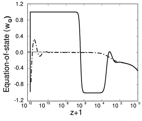
FIG. 4.: The convergence of different initial conditions to the tracker solution. As derived in the text, $w_{Q}$ decays exponentially fast to the tracker solution combined with small oscillations. All the curves are for $V(Q)=M^{4}/Q^{6}$. The solid curve is the overshoot case from Figure 1. The thin dashed curve with $w\approx 0$ is the tracker solution which is overlaid for most $z$ by the dash-dotted curve, which represents a slightly undershooting solution.

In deriving Eq. (16), we have assumed that $\Gamma$ is strictly constant, independent of $Q$, which is exactly true for pure inverse power-law ($V\sim 1/Q^{\alpha}$) or exponential ($V\sim{\rm exp}(\beta Q)$) potentials. The same result holds if $|d(\Gamma-1)/Hdt|/|\Gamma-1|\ll 1$ (i.e., $\Gamma-1$ varies with $Q$ but only by a modest amount) over the plausible range of initial conditions ranging from $V(Q)\approx\rho_{Bi}$ to $V(Q)\approx\rho_{eq}$ (where $\rho_{Bi}$ is the initial background energy density after inflation, say, and $\rho_{eq}$ is the energy density at matter-radiation equality). The condition is equivalent to $|\Gamma^{\prime}/[\Gamma\,(V^{\prime}/V)]|\ll 1$. In this limit, $\Gamma$ and the tracker value of $w_{Q}$ change adiabatically as $Q$ rolls downhill, satisfying the tracker equation with $\dot{x}$ being negligibly small, as discussed in the Appendix. The constraints on $w_{Q}$ are the same as above. However, some important differences from the constant $\Gamma$ case are pointed out in the last section.

Throughout most of our discussion in this paper, we have considered the case $w_{Q}<w_{B}$. However, our convergence criterion, $w_{0}<\frac{1}{2}(1+w_{B})$, includes $w_{Q}>w_{B}$ or, equivalently, $1-(1-w_{B})/(6+2w_{B})<\Gamma<1$, as also found by Liddle and Scherrer.[16] An example is $V\sim Q^{\alpha}$ with $\alpha\geq(6+2w_{B})/(1-w_{B})$; $\alpha\geq 6$ for $w_{B}=0$ and $\alpha\geq 10$ for $w_{B}=1/3$. Let us suppose we reached the present $\Omega_{Q}$ after tracking down this potential. Because $w_{Q}>w_{B}$ in these potentials, it must be that $\Omega_{Q}$ exceeds $\Omega_{B}$ extrapolating backwards in time. Consequently, there is no period of matter-domination or structure formation, and these models have no practical interest. However, see the discussion of hybrid models below for a variation on these models that may be viable.

G Borderline models and hybrid models

For completeness, we consider two special classes of potentials, borderline trackers in which $\Gamma=1$ and hybrid models in which $\Gamma>1$ at first and then $\Gamma<1$.

The borderline case corresponds to $V\propto{\rm exp}(\beta Q)$, which has been studied by several authors.[6, 7, 10, 11] For this case, the tracker equation for $\dot{x}=\ddot{x}=0$ demands that $w_{Q}=w_{B}$ and, therefore, $\Omega_{Q}$ is constant. Hence, for this case, the tracker solution corresponds to maintaining a constant ratio of quintessence to background energy density. The only deviation occurs during the transition from radiation- to matter-domination when $\dot{x}$ becomes non-negligible, but this is a small effect.

Because $\Omega_{Q}$ is constant throughout the matter-dominated epoch, these models have limited practical utility. $\Omega_{Q}$ must be small ($\leq 15\%$) at the onset of matter-domination in order not to disrupt structure formation. (Quintessence suppresses the growth rate.) But, then, since $\Omega_{Q}$ is constant, $\Omega_{Q}$ remains small forever. Consequently, the models require $\Omega_{m}>85\%$, inconsistent with a number of determinations of mass[15], and the universe never enters a period of accelerated expansion, inconsistent with recent measurements of the luminosity-red shift relation for Type IA supernovae.[18] (The overshoot scenario may lift the $\Omega_{m}>85\%$ constraint but, as discussed in Section D, introduces fine tuning which defeats the whole purpose of the scenario.)

Hybrid models have the property that solutions converge to a tracker solution at the early phase of evolution but cease to converge after a certain point due to a change in the shape of the potential as $Q$ rolls downhill. One can imagine a sufficiently long convergence regime that all or most plausible initial conditions have collapsed to a common tracker solution before the second regime begins. Effectively, this has the desired feature that a wide range of initial conditions lead to the same final condition. The models may be somewhat artificial in that the current cosmology is very sensitive to where the transition occurs. For example, consider the case where $w_{Q}<w_{B}$ but $\Gamma$ undergoes a transition from $\Gamma>1$ (converging) to $\Gamma<1$. Recall that $\Gamma<1$ corresponds to $|V^{\prime}/V|$ increasing as $V$ decreases. We have shown that, extrapolating backwards only a small interval in time, the field $Q$ must have been frozen at a value not so different from the current value (assuming the field is rolling today and $w_{Q}<0$). In this kind of hybrid model, the transition to $\Gamma<1$ must be set so that the transition occurs so that $Q$ is near the frozen value, which requires delicate tuning of parameters in the potential.

A different example is where $1-(1-w_{B})/(6+2w_{B})<\Gamma<1$ and $w_{Q}>w_{B}$ during the early stages of the universe. We have argued that these conditions produce converging behavior but, if the conditions continue to the present, there is no period of matter-domination or structure formation (see Section III.F). However, one can imagine hybrid models in which these conditions $[1-(1-w_{B})/(6+2w_{B})]<\Gamma<1$ and $w_{Q}>w_{B}$ are satisfied for some period early in the history of the universe, providing a finite period of converging behavior. Later, as $Q$ moves down the potential, $V$ changes form so that $w_{Q}<w_{B}$. Viable cosmological models of this type can be constructed in which $\Omega_{Q}$ does not dominate the universe during the matter-dominated epoch until near the present time.

H Some additional practical considerations

We have discovered a wide class of potentials that exhibit tracking behavior. This guarantees that a wide range of initial conditions converge to a common tracking solution, but the convergence may take longer than the age of the universe in some cases. In particular, if one assume equipartition after inflation, say, and the initial $V$ is too far above the tracker solution, then $Q$ falls precipitously, overshoots the tracker solution, and freezes at some $Q=Q_{f}$. For some potentials satisfying the condition $\Gamma\approx\,{\rm constant}\,>1$, $Q_{f}$ may be so large that the field does not begin to roll and track by the present epoch. If $Q$ just started to roll by the present epoch, then it would behave exactly as a cosmological constant until now, and so the model is trivially equivalent to a $\Lambda$ model. As a practical consideration, we demand that a field starting from equipartition initial conditions should start rolling by matter-domination, say, so that the model is non-trivial. This imposes a mild added constraint on potentials, $V(Q)$. For this purpose, rough estimates suffice.

Equipartition at the end of inflation, when there are hundreds or perhaps thousands of degrees of freedom in the cosmological fluid, means that the $Q$-field has $\Omega_{i}\approx 10^{-3}$. Beginning from equipartition, $Q$ falls to some value $Q_{f}$ where it freezes. According to the equation-of-motion, $Q$ remains frozen until $\sqrt{\Omega_{Q}}\propto\sqrt{V}/H$ increases to where $V^{\prime}/V\sim 1/\sqrt{\Omega_{Q}}$ or, equivalently,

$$\frac{V^{\prime 2}}{V}(Q_{f})>H^{2}(z_{eq})=\frac{H_{0}^{2}}{a^{3}_{eq}}\sim\frac{1}{\Omega_{0}}\frac{V_{0}}{a^{3}_{eq}}.$$ (18)

For $V(Q)\propto 1/Q^{\alpha}$, this imposes the constraint

$$\frac{\alpha^{2}}{Q_{f}^{\alpha+2}}\geq\frac{1}{\Omega_{0}\,Q_{0}^{\alpha}\,a^{3}_{eq}},$$ (19)

where $Q_{0}$ is the present value of $Q$. Since today

$$\frac{V_{0}^{\prime 2}}{V_{0}}\sim H_{0}^{2}\sim\frac{8\pi}{3}\frac{V_{0}}{\Omega_{0}},$$ (20)

we obtain $Q_{0}^{2}\sim\frac{3}{8\pi}\Omega_{Q}^{0}\alpha^{2}$. From Eq. (12), we also know that

$$\frac{4\pi}{3}Q_{f}^{2}\sim\Omega_{i}\sim 10^{-3}.$$ (21)

Combining the above relations one gets the restriction on $\alpha$

$$\alpha^{2}>\frac{10^{12}}{\Omega_{0}}\frac{(\frac{3}{4\pi}\Omega_{i})^{(1+\alpha/2)}}{(\alpha^{2}\Omega_{0}\frac{3}{8\pi})^{\alpha/2}}$$ (22)

where we have taken $a_{eq}\sim 10^{-4}$. This approximate relation leads to $\alpha\geq 5$. Figure 5 confirms this result showing that the $\alpha=1$ model starts rolling much later than equality. So, if one restricts to pure inverse power-law ($1/Q^{\alpha}$) potentials, our constraint that $Q$ begin from equipartition and roll before matter-radiation equality constrains us to $\alpha\geq 5$.

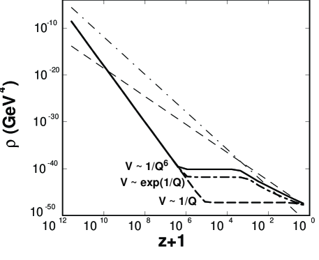
FIG. 5.: A comparison of the overshoot for three different models beginning from $\Omega_{i}=10^{-3}$ (equipartition). The thick solid line is for $V(Q)=M^{4}/Q^{6}$, the thick dash-dotted line is for $V=M^{4}[exp(1/Q)-1]$, and the thick long dashed line is for $V(Q)=M^{4}/Q$. In all three examples, $Q$ falls rapidly downhill and freezes. In the first and second examples, $Q$ begins to roll again and joins the tracker solution before matter-radiation equality; the third example, which violates the condition derived in the text, does not begin to roll again by the present epoch.

IV The $\Omega_{Q}$-$w_{Q}$ relation

An extremely important aspect of tracker solutions is the $\Omega_{Q}$-$w_{Q}$ relation, or, equivalently, the $\Omega_{m}$-$w_{Q}$ relation which it forces. For any given $V=M^{4}\tilde{v}(Q/M)$ (where $\tilde{v}$ is a dimensionless function of $Q/M$), $Q$ and $\dot{Q}$ are totally determined independent of initial conditions by the tracker solution. The only degree of freedom is the $M$-parameter in the potential. $M$ can be fixed by imposing the constraint that the universe is flat and $\Omega_{m}=1-\Omega_{Q}$ is determined by measurement. There is, then, no freedom left to independently vary $w_{Q}$. This is the explanation of the $\Omega_{Q}$-$w_{Q}$ relation, a new prediction that arises from tracker fields. The $\Omega_{Q}$-$w_{Q}$ relation is not unique because there remains the freedom to change the functional form of $V(Q)$. Even so, $w_{Q}$ is sufficiently constrained as to be cosmologically interesting.

The general trend is that $w_{Q}\rightarrow-1$ as $\Omega_{Q}\rightarrow 1$. The fact that $\Omega_{m}\geq 0.2$ observationally means that $\Omega_{Q}\leq 0.8$ and $w_{Q}$ cannot be very close to $-1$. How small $w_{Q}$ can be is model-dependent. We are most interested in the smallest values of $w_{Q}$ possible since the difference from $-1$ determines how difficult it is to distinguish the tracking field candidate for missing energy from cosmological constant.

In Figure 6, we show the $\Omega_{Q}$-$w_{Q}$ relation for a series of pure, inverse power-law potentials, $V(Q)\propto 1/Q^{\alpha}$. The general trend is that $w_{Q}$ increases as $\alpha$ decreases. The constraint given at the end of the previous section is that $\alpha\geq 5$ (in order that $Q$ be rolling by matter-radiation equality beginning from equipartition initial conditions). For $\Omega_{Q}=0.8$, the smallest value of $w_{Q}$ is -0.52, which occurs for $\alpha=5$. This is a large difference from $-1$ obtained for a cosmological constant.

However, a lower value of $w_{Q}$ can be easily achieved for a more generic potential with a mixture of inverse power-laws, e.g., $V(Q)=M^{4}\,{\rm exp}(1/Q)$. For these models, $Q$ is small initially. If the potential is expanded in inverse powers of $Q$, $1/Q^{\alpha}$, then it is dominated in the early stages by the high-$\alpha$ terms. Hence, the effective value of $\alpha$ is much greater than 5 before matter-radiation equality, and we easily satisfy the constraint that the field be rolling before matter-radiation equality beginning from equipartition initial conditions. On the other hand, the value of $Q$ at the present epoch is large, and the potential is dominated by the $\alpha\approx 1$ terms in its expansion. Consequently, $w_{Q}$ can be even lower today than in the pure power-law case. For $\Omega_{Q}=0.8$, we obtain $w_{Q}=-0.72$ for the exponential potential, which is in better accord with recent constraints on $w_{Q}$ from supernovae.[18]

It is difficult to go below this limit without artificially tuning potentials unless we relax our constraints. For example, consider the highly contrived potential $V(Q)=\frac{A}{Q^{10^{-5}}}+\frac{B}{Q^{10}}$, in which we have intentionally chosen exponents differing by six orders of magnitude in order to obtain a small $w_{Q}$ today. The second term in the potential dominates before equality and insures that the field is rolling by that point in time. The first term dominates at late times and makes the equation of state $w_{0}$ very low (because this term is very flat). For this example, we find $w_{Q}=-0.98$ for $\Omega_{Q}=0.8$. However, we had to choose a pair of terms with exponents differing by six orders of magnitude. The lesson of this exercise (and related tests) is that the exponential potential is a reliable estimate for the minimal $w_{Q}$ possible for generic, untuned potentials.

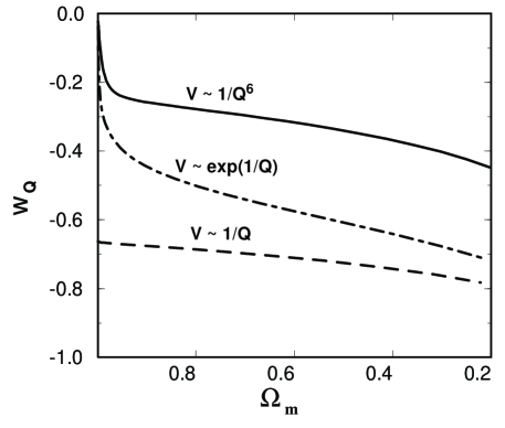
FIG. 6.: The $\Omega_{Q}$-$w_{Q}$ relation for various potentials assuming a flat universe $\Omega_{m}=1-\Omega_{Q}$, where $w_{Q}$ represents the present value of $w_{Q}$. The potentials and notation are the same as in Figure 5.

In Figure 6, we illustrate the $\Omega_{Q}$-$w_{Q}$ relation for several potentials. Only the $V\sim 1/Q^{6}$ and $V\sim{\rm exp}(1/Q)$ potentials satisfy the condition that $Q$ is rolling by matter-radiation equality beginning from equipartition initial conditions. In Figure 7, we illustrate the effective $w_{Q}^{eff}$ that would be measured using supernovae or cosmic microwave background measurements, using the $V\sim{\rm exp}(1/Q)$ potential as defining the boundary of minimal values of $w_{Q}$ possible for the tracker field case. This boundary assumes that we satisfy the strict condition that the field be rolling by matter-radiation equality beginning from equipartition initial conditions. If we relax this condition and allow a somewhat narrower range of initial conditions, then general potentials of the form $V\sim\Sigma c_{k}/Q^{k}$ (such as $V\sim 1/Q$) are allowed and $w_{Q}$ can be somewhat smaller (see Figure 6). Hence, in Figure 7, the boundary can relax somewhat downward (dashed line) but it is difficult to obtain $w_{Q}<-0.8$ or $w_{Q}^{eff}<-0.75$. Because $w_{Q}$ is evolving at recent times, the value obtained from measurements at moderate to deep red shift will differ from the current value shown in Figure 6. For tracker potentials, the effect of integrating back in time over varying $w_{Q}$ turns out to be well-mimicked by a model with constant $w_{Q}=w_{Q}^{eff}$ that has the same conformal distance to last scattering surface. For the case $\Omega_{m}=0.2$, for example, Figure 6 shows that $w_{Q}=-0.72$ today, but Figure 7 shows that the measured $w_{Q}$ would be $w_{eff}=-0.63$.

The result is exciting because the $\Omega_{Q}$-$w_{Q}$ relation and the constraint on $\Omega_{m}\geq 0.2$ today creates a sufficiently large gap between $w_{Q}^{eff}$ and $-1$ that the tracker candidate for missing energy should be distinguishable from the cosmological constant in near-future cosmic microwave background and supernovae measurements.

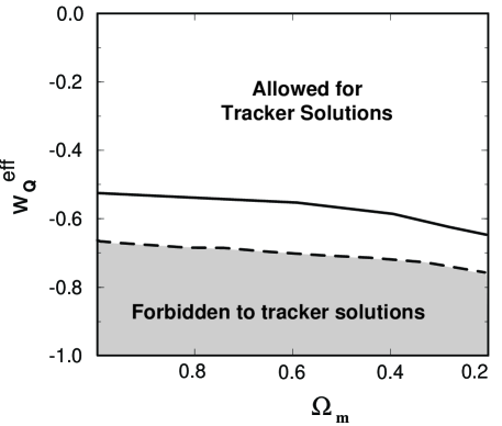
FIG. 7.: A plot of $w_{Q}^{eff}$ versus $\Omega_{m}=1-\Omega_{Q}$, showing the minimum $w_{Q}^{eff}$ possible for tracker solutions. The solid line is the lower boundary assuming the constraint that the $Q$-field begins with equipartition initial conditions and begins rolling before matter-radiation equality. The dashed line is the lower boundary if this condition is relaxed to allow general $V\sim\Sigma c_{k}/Q^{k}$. As explained in the text, $w_{Q}^{eff}$ is the value that would be measured in supernovae and microwave background experiments which effectively integrate over a varying $w_{Q}$.

V Why is the universe accelerating today?

We have proven in this paper that tracker potentials resolve the coincidence problem for quintessence. For a very wide range of initial conditions, cosmic evolution converges to a common track. The tracker models are similar to inflation in that they funnel a diverse range of initial conditions into a common final state. The models have only one important free parameter ($M$) which is fixed by the measured $\Omega_{Q}=1-\Omega_{m}$.

Some of the mathematical properties of tracking solutions have been noted before for ${\rm exp}(\beta Q)$ and pure, inverse power-law potentials.[6, 7, 10, 11] However, the extraordinary insensitivity to initial conditions and the potential application to the coincidence problem was not explored. The present work is important because it shows that the properties are shared by a much wider class of more generic potentials. “Generic potentials” include, for example, all $V$’s which can be expanded as a finite or infinite sum of terms with inverse powers of $Q$, which is much more general than the special cases of a single inverse-power or a pure exponential. We use $V=M^{4}\,{\rm exp}(1/Q)$ as an example of this more generic class, although our conclusions would remain the same for more general $V=\Sigma c_{k}/Q^{k}$.

Extending the tracker behavior to generic potentials may be important because, as we shall argue below, they have properties not shared by the special cases ($V\sim 1/Q^{\alpha}$ and $V\sim{\rm exp}(\beta Q)$) that make plausible why $\Omega_{Q}$ only begins to to dominate and initiate a period of accelerated expansion late in the history of the universe.

To understand this conclusion, we need to change our approach. Up to this point in the paper, we have imagined fixing $M$ to guarantee that $\Omega_{Q}=1-\Omega_{m}$ has the measured value today. This amounts to considering one tracker solution for each $V(Q)$. Now we want to consider the entire family of tracker solutions for each given $V(Q)$ and consider whether $\Omega_{Q}$ is more likely to dominate late in the universe for one $V(Q)$ or another.

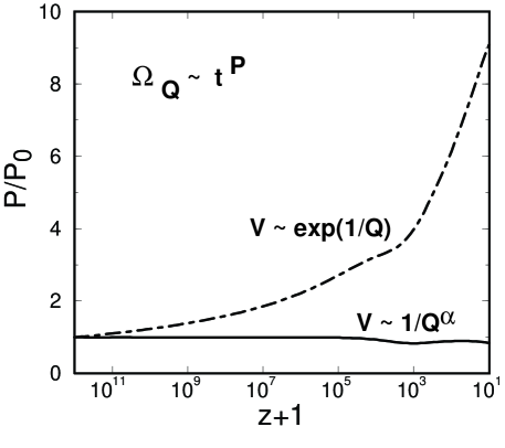
FIG. 8.: A plot of $P/P_{0}$ versus $t$, where $\Omega_{Q}\propto t^{P}$ and $P_{0}$ is the initial value of $P$. The plot compares pure inverse power-law ($V\sim 1/Q^{\alpha}$) potentials for which $P$ is constant with a generic potential (e.g., $V\sim{\rm exp}(1/Q)$) for which $P$ increases with time.

In general, $\Omega_{Q}$ is proportional to $a^{3(w_{B}-w_{Q})}\propto t^{2(w_{B}-w_{Q})/(1+w_{B})}$, where we have shown in Eq. (9) that

$$w_{B}-w_{Q}=\frac{2(\Gamma-1)(w_{B}+1)}{1+2(\Gamma-1)}.$$ (23)

Hence, we find $\Omega_{Q}\propto t^{P}$ where

$$P=\frac{4(\Gamma-1)}{1+2(\Gamma-1)}.$$ (24)

A satisfying explanation as to why $\Omega_{Q}$ dominates at late times, rather than early, would be if $\Omega_{Q}$ automatically changes behavior at late times. This is not the case for the two special cases ($V\sim 1/Q^{\alpha}$ and $V\sim{\rm exp}(\beta Q)$). As the universe evolves, $\Gamma-1$ and, hence, $P$ are constant; consequently, $\Omega_{Q}$ grows as the same function of time throughout the radiation- and matter-dominated epochs. However, these are the exception, rather than the rule.

For more general potentials, $P$ increases as the universe ages. Consider first a potential which is the sum of two inverse power-law terms with exponents $\alpha_{1}<\alpha_{2}$. The term with the larger power is dominant at early times when $Q$ is small, but the term with the smaller power dominates at late times as $Q$ rolls downhill and obtains a larger value. Hence, the effective value of $\alpha$ decreases and $\Gamma-1\propto 1/\alpha$ increases; the result is that $P$ increases at late times. For more general potentials, such as $V\sim{\rm exp}(1/Q)$, the effective value of $\alpha$ decreases continuously and $P$ increases with time. Figure 8 illustrates the comparison in the growth of $P$.

How does this explain why $\Omega_{Q}$ dominates late in the universe? Because an increasing $P$ means that $\Omega_{Q}$ grows more rapidly as the universe ages. Figure 9 compares a tracker solution for a pure inverse power-law potential ($V\sim 1/Q^{6}$) model with a tracker solution for $V\sim{\rm exp}(1/Q)$, where the two solutions have been chosen to begin at the same value of $\Omega_{Q}$. (The start time has been chosen arbitrarily at $z=10^{17}$ for the purposes of this illustration.) Following each curve to the right, there is a dramatic (10 orders of magnitude) difference between the time when the first solution (solid line) meets the background density versus the second solution (dot-dashed line). That is, beginning from the same $\Omega_{Q}$, the first tracker solution dominates well before matter-radiation equality and the second (generic) example dominates well after matter-domination. The difference is less dramatic as $\alpha$ increases for the pure inverse power-law model and becomes negligible for $\alpha>15$. Of course, the model appears more contrived. But, more importantly, as $\alpha$ increases, the value of $w_{Q}$ today (given $\Omega_{m}\geq 0.2$) approaches zero and the universe does not enter a period of acceleration by the present epoch. Hence, a significant conclusion is that the pure exponential and inverse power-law models are atypical; the generic potential has properties that make it much more plausible that $\Omega_{Q}$ dominates late in the history of the universe and induces a recent period of accelerated expansion.

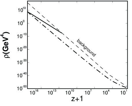
FIG. 9.: A plot comparing two tracker solutions for the case of a $V\sim 1/Q^{6}$ potential (solid line) and a $V\sim{\rm exp}(1/Q)$ potential (dot-dash). The dashed line is the background density. The two tracker solutions were chosen to have the same energy density initially. The tracker solution for the generic example ($V\sim{\rm exp}(1/Q)$) reaches the background density much later than for the pure inverse-power law potential. Hence, $\Omega_{Q}$ is more likely to dominate late in the history of the universe in the generic case.

In sum, the general tracker behavior shown in this paper goes a long way towards resolving two key issues: the coincidence (or initial conditions) problem and why $\rho_{Q}$ is dominating today rather than at some early epoch. And, it leads to a new prediction – a relation between $\Omega_{m}=1-\Omega_{Q}$ and $w_{Q}$ today that makes tracker fields distinguishable from a cosmological constant.

We wish to thank Robert Caldwell and Marc Kamionkowski for many insightful comments and suggestions. This research was supported by the US Department of Energy grants DE-FG02-92-ER40699 (Columbia) DE-FG02-95ER40893 (Penn) and DE-FG02-91ER40671 (Princeton).

VI Appendix

In this Appendix, we discuss the convergence to the tracker solution when $\Gamma\equiv V^{\prime\prime}V/(V^{\prime})^{2}$ varies with $Q$. We wish to show that convergence occurs if the variation of $\Gamma$ over the plausible range of initial conditions (varying of 100 orders of magnitude in energy density) is nearly constant. An example is $V\sim{\rm exp}(1/Q)$ for which $\Gamma=1+2Q$ and $Q\ll 1$ for the plausible range of initial conditions.

The condition that $\Gamma$ is nearly constant means precisely that $d(\Gamma-1)/Hdt\ll(\Gamma-1)$ or, equivalently, $|\Gamma^{\prime}/[\Gamma\,(V^{\prime}/V)]|\ll 1$. In this case, $\Gamma$ is nearly constant over a Hubble time. Hence, we can consider an adiabatic approximation for the tracker solution in which $Q_{0}$ and $w_{0}$ satisfy the tracker equation Eq. (6) with $\dot{x}$ and $\ddot{x}$ negligibly small. Suppose $w_{Q}$ and $Q$ are both perturbed from this tracker solution by amounts $\delta w$ and $\delta Q(t)$. From the definition of $w_{Q}$, we have that

$$\delta w=(1-w_{0})\frac{\dot{Q}_{0}}{\rho_{0}}\delta\dot{Q}-(1+w_{0})\frac{V_{0}^{\prime}}{\rho_{0}}\delta Q.$$ (25)

From the equation-of-motion Eq. (4) we know that

$$\frac{V_{0}^{\prime}}{\rho_{0}}\sim\frac{V^{\prime}_{0}}{V_{0}}\propto\frac{1}{\sqrt{\Omega_{Q}}}\propto a^{-3(w_{Q}-w_{B})}.$$ (26)

Consequenty, Eq. (25) implies

$$\delta w\sim{\rm exp}\,[-3/2(w_{B}-w_{0})\ln{a}]\,\delta Q.$$ (27)

In particular, this equation shows that $\delta w$ decays if $\delta Q$ decays.

To show the $\delta Q$ decays, we start from the more standard form of the equation-of-motion:

$$\ddot{Q}+3H\dot{Q}+V^{\prime}=0,$$ (28)

and obtain the perturbed equation

$$\delta\ddot{Q}+3H\delta\dot{Q}+V_{0}^{\prime\prime}\delta Q=0.$$ (29)

Changing the variable to $d\tau=Hdt$, we obtain

$$\frac{d^{2}\delta Q}{d\tau^{2}}=\frac{d}{Hdt}\left(\frac{d\delta Q}{Hdt}\right)=\frac{1}{H^{2}}\ddot{Q}+m\frac{d\delta Q}{d\tau}$$ (30)

where $m\equiv(Ht)^{-1}=3(w_{B}+1)/2$. Eq. (29) then becomes

$$\frac{d^{2}\delta Q}{d\tau^{2}}+(3-m)\frac{d\delta Q}{d\tau}+\frac{V_{0}^{\prime\prime}}{H^{2}}\delta Q=0.$$ (31)

where

$$C\equiv\frac{V_{0}^{\prime\prime}}{H^{2}}\approx\frac{9}{4}(1-w_{Q})(2+w_{B}+w_{Q})$$ (32)

in the adiabatic approximation. The solution to Eq. (31) is $\delta Q=A\exp{(\beta\tau)}$, where

$$\beta^{2}+(3-m)\beta+C=0$$ (33)

with solutions

$$\beta_{\pm}=-\frac{B}{2}\left[1\pm\sqrt{1-\frac{4C}{B^{2}}}\right]$$ (34)

where

$$B=3-m=\frac{3}{2}(1-w_{B}).$$ (35)

Note that $B>0$ and $C>0$. Hence, we have that $\delta Q$ exponentially decays, and, by the argument that preceded, $\delta w\propto\delta Q$ also decays exponentially. Combining our relations for $\delta Q$ and $\delta w$, we can reproduce the result in Eq. (16) obtained for the constant $\Gamma$ case.

If $Q$ has spatial fluctuations, Eq. (31) must be modified by a positive term proportional to $k^{2}\delta Q$. The effect is to increase $C$ and modify the oscillation frequency. However, the exponential suppression of the fluctuations is retained once the field starts approaching the attractor solution. Hence, even if the initial conditions result in significant fluctuations after the field is frozen (in either the undershoot or overshoot case), the initial fluctuations are erased as $Q$ converges to the tracker solution.

REFERENCES

- [1] R.R. Caldwell, R. Dave and P.J. Steinhardt, Phys. Rev. Lett. 80, 1582 (1998).
- [2] See, for example, J. P. Ostriker and P.J. Steinhardt, Nature 377, 600 (1995), and references therein.
- [3] M. S. Turner, G. Steigman, and L. Krauss, Phys. Rev. Lett. 52, 2090 (1984)
- [4] M.S. Turner, and M. White, Phys. Rev. D 56, R4439 (1997).
- [5] N. Weiss, Phys. Lett. B 197, 42 (1987).
- [6] B. Ratra, and P.J.E. Peebles, Phys. Rev. D 37, 3406 (1988); P.J.E. Peebles and and B. Ratra, ApJ 325, L17 (1988).
- [7] C. Wetterich, Astron. Astrophys. 301, 32 (1995).
- [8] J.A. Frieman, et al. Phys. Rev. Lett. 75, 2077 (1995).
- [9] K. Coble, S. Dodelson, and J. Frieman, Phys. Rev. D 55, 1851 (1995).
- [10] P.G. Ferreira and M. Joyce, Phys. Rev. Lett. 79, 4740 (1997); Phys. Rev. D 58, 023503 (1998).
- [11] E. J. Copeland, A.R. Liddle, and D. Wands, Phys. Rev. D57, 4686 (1998).
- [12] P. Steinhardt, in ‘Critical Problems in Physics,” ed. by V.L. Fitch and D.R. Marlow (Princeton U. Press, 1997).
- [13] R.H. Dicke and P.J.E. Peebles, in General Relativity: An Einstein Centenary Survey, ed. by S.W. Hawking & W. Israel (Cambridge U. Press, 1979).
- [14] I. Zlatev, L. Wang and P. J. Steinhardt, astro-ph/9807002.
- [15] L. Wang, R.R. Caldwell, J.P. Ostriker, and P.J. Steinhardt, in preparation.
- [16] A. Liddle and R. Scherrer, astro-ph/9809272.
- [17] P. Binetruy, hep-ph/9810553.
- [18] S. Perlmutter, et al, astro-ph/9812133; A. G. Riess, et al, astro-ph/9805201; P. M. Garnavich et al, astro-ph/9806396.
- [19] G. W. Anderson and S. M. Carroll, astro-ph/9711288.
- [20] T. Barreiro, B. de Carlos, E.J. Copeland, Phys.Rev. D57, 7354 (1998).
- [21] P. Binetruy, M. K. Gaillard, Y.-Y. Wu, Phys. Lett. B412, 288 (1997); Nucl. Phys. B493, 27 (1997).
- [22] J.D. Barrow, Phys. Lett. B235, 40 (1990).
- [23] C. Hill, and G.G. Ross, Nuc. Phys. B 311, 253 (1988); Phys.Lett. B 203, 125 (1988).
- [24] I. Affleck, M. Dine, and N. Seiberg, Nuc. Phys. B 256, 557 (1985).