INVESTIGATING THE METAL LINE SYSTEMS AT z=1.9 TOWARD J2233$-$606 IN THE HDF-S

Abstract

The combination of STIS and optical spectroscopy with STIS imaging of the field surrounding J2233$-$606 afford a unique opportunity to study the physical nature of the Quasar Absorption Line systems. We present an analysis of the ionization state, chemical abundances, and kinematic characteristics of two metal-line systems at $z=1.92$ and $z=1.94$ toward J2233$-$606. We focus on these two systems because (i) the observations provide full coverage of the Lyman series, hence an accurate determination of their HI column densities and (ii) they exhibit many metal-line transitions which allow for a measurement of their ionization state and chemical abundances.

Line-profile fits of the Lyman series for the two systems indicate $\log{N({\rm HI})}=17.15\pm 0.02\,{\rm cm^{-2}}$ evenly distributed between two components for the $z=1.92$ system and $\log{N({\rm HI})}=16.33\pm 0.04\,{\rm cm^{-2}}$ for the $z=1.94$ system. By comparing observed ionic ratios of C and Si against calculations performed with the CLOUDY software package, we find the ionization state is high and well constrained in both systems. Applying ionization corrections to the measured ionic column densities, we determine that the systems exhibit significantly different metallicities: $\approx 1/50$ solar and $<1/200$ solar for the two components of $z=1.92$ and $\approx 40\%$ solar at $z=1.94$. The properties of the $z=1.92$ system are consistent with a low metallicity galaxy (e.g. a dwarf galaxy) as well as absorption by large scale structure of the IGM. On the other hand, the high metallicity of the $z=1.94$ system suggests significant star formation and is therefore most likely associated with a galactic system. Furthermore, we predict it is the most likely to be observed with the STIS imaging and follow-up observations. If a galaxy is identified, our results provide direct measurements on the properties of the ISM for a $z\approx 2$ galaxy.

1. INTRODUCTION

Identifying the physical nature of the Quasar Absorption Line (QAL) systems will have significant impact on our understanding of galaxy formation, chemical evolution, and large scale structure (LSS). At high redshift, where QAL systems offer one of the most efficient means of probing the early universe, any insight is notable. To really utilize QAL samples as tools to study cosmology (LSS, dN/dz) and early galaxy formation, we need to relate the absorbers to astrophysical environments and objects. With the advancement of modern telescopes and instrumentation, in particular high resolution echelle spectroscopy, observers are now accurately examining the physical characteristics of these systems. For the damped Ly$\alpha$ systems, the metallicity (Pettini et al. (1997)), abundance patterns (Lu et al. (1996); Prochaska & Wolfe (1999)) and kinematic characteristics (Prochaska & Wolfe 1997b ; Prochaska & Wolfe (1998)) have been well studied and have revealed vital clues to their physical nature.

Table 1Spectroscopic Data

Instrument/Telescope	Coverage	Resolution	Source
E230M-STIS/HST	2300$-$3100 Å	$R=30000$	HST HDF-S STIS Team
G430M-STIS/HST	2300$-$3100 Å	0.56 å	HST HDF-S STIS Team
UCLES/AAT	3530$-$4390 Å	$R=35000$	Outram et al. (1998)
EMMI/NNT	4386$-$8270 Å	14 km/s	Savaglio (1998)

Recent observations of the Hubble Deep Field South afford a unique opportunity to investigate the physical nature of the QAL systems. With the combination of STIS spectroscopy and STIS imaging (Gardner et al. (1999); Williams et al. (1999)) of the field toward J2233$-$606 ($z_{em}=2.238$, $B=17.5$; Boyle (1997)) researchers may directly identify the absorbers responsible for the QAL systems. In turn, these observations will further develop the relationship between QAL systems and galaxies or large scale structure at moderate redshift. In this paper, we investigate the physical properties of the two metal line systems at $z\approx 1.9$ toward J2233$-$606. We choose these two systems because the STIS spectroscopy coupled with optical echelle spectroscopy of J2233$-$606 (Outram et al. (1998); Savaglio (1998)) allows one to well constrain the ionization state of these systems. By applying ionization corrections to the measured ionic column densities, we present chemical abundances for Si, C, N, and Fe. Finally, we comment on the kinematic characteristics of the absorption line systems and speculate on the systems’ association with protogalaxies and large scale structure at high redshift.

In $\S$ 2, we discuss the multiple data sets used in this analysis. Section 3 details our fits to the Lyman series of the two QAL systems. The ionic column densities, ionization state, and chemical abundances are examined in $\S$ 4. Finally, we speculate on the impact of these measurements in $\S$ 5.

2. DATA

In the following analysis we utilize several data sets obtained with a number of instruments and telescopes (Table 1). These include ultra-violet spectra taken with the STIS E230M echelle and G430M grating on board the Hubble Space Telescope, and optical echelle spectroscopy acquired with the AAT and NTT and kindly provided by Outram et al. (1998) and Savaglio (1998). In all, this collection of data provides continuous coverage from $2275-8300$Å  with resolution $R\approx 30000$ (except the region from $3100-3500$Å  corresponding to the G430M grating) and moderate signal to noise (S/N). With the exception of the NTT spectrum where we have adopted the continuum provided by Savaglio, we have continuum fit the spectra with low order Legendre polynomials using a package similar to the Iraf routine continuum.

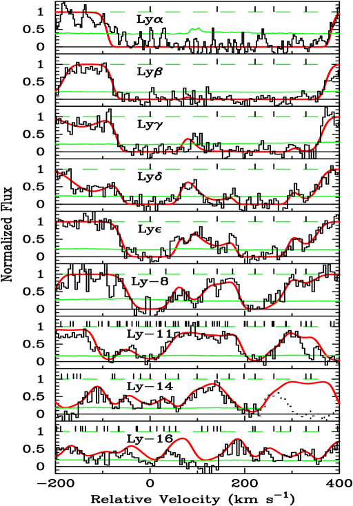
Figure 1.— A plot of the Lyman series for the Lyman limit system at $z=1.92$ toward J2233$-$606. Overplotted is the VPFIT solution which includes several coincident Ly$\alpha$ forest clouds. The dotted regions indicate data not included in our fit to the Lyman series.

3. HI MEASUREMENTS

A requisite facet in analyzing the ionization state and chemical abundances of QAL systems is an accurate determination of the HI column density. For the QAL systems at $z=1.92$ and $z=1.94$ towards J2233$-$606, the echelle observations performed with STIS on board the HST are essential as they allow for a fit to the higher order lines in the Lyman series. We have measured the HI column densities by fitting Voigt profiles to the Lyman series with the VPFIT package kindly provided by R. Carswell and J. Webb. Figures 1 and 2 and Table 2 present the results of this analysis. Note that in performing the fit to the Lyman series, we have included fits to other Ly$\alpha$ forest clouds when necessary.

In the z=1.92 system, most of the H I is split between two main components at $z=$1.9256290 and 1.9279202. The total column density is $\log{N({\rm HI})}=17.15\pm 0.02\,{\rm cm^{-2}}$ with a nearly even split between the main components. As suggested by Outram et al. (1998), the STIS observations clearly demonstrate that the Lyman break evident at $\approx 2700$ Å  is due to the Lyman limit (LL) system at $z=1.92$. For the z=1.94 system, the majority of H I falls at z=1.9425817 and the column density is well constrained by the high-order unsaturated Lyman lines (Ly-10, 11, 12). We find $\log{N({\rm HI})}=16.33\pm 0.04\,{\rm cm^{-2}}$. Therefore this system has a minimal contribution to the observed Lyman break.

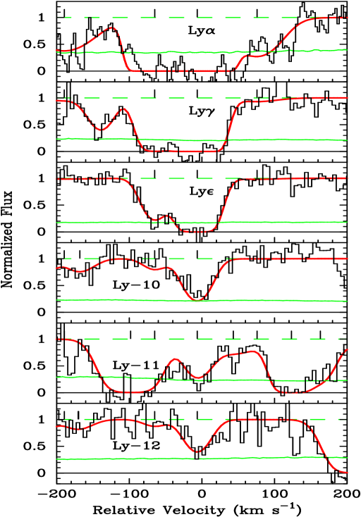
Figure 2.— A plot of the Lyman series for the QAL system at $z=1.94$ toward J2233$-$606. Overplotted is the VPFIT solution which includes several coincident Ly$\alpha$ forest clouds. The dotted regions indicate data not included in our fit to the Lyman series.

Only weak limits can be placed on D/H in these absorption systems. In the z=1.94 system, extra H I falls to the blue of the main H I component (at $-$60 km/s) making future detection of the D I line impossible. In the z=1.92 system, the Ly$\alpha$ line is too wide for a detection or an upper limit. The blue wing of Ly$\beta$ might be used for an upper limit, but only a weak limit is derived from the STIS E230M spectrum: D/H $<10^{-3}$.

Table 2

HI FITS FOR THE Z=1.92 AND Z=1.94 QAL SYSTEMS $z_{abs}$ log $N$ $\sigma_{logN}$ $b$ $\sigma_{b}$ ($\,{\rm cm^{-2}}$) ($\,{\rm cm^{-2}}$) (km s^-1 ) (km s^-1 ) 1.2574902 12.93 0.17 8.1 4.0 1.2847255 13.81 0.05 48.5 6.4 1.3393718 13.28 0.09 42.6 10.2 1.3529782 13.42 0.07 21.1 3.8 1.4667628 13.77 0.06 24.9 2.5 1.9407216 13.80 0.09 49.2 6.1 1.9419496 15.46 0.06 20.3 1.6 1.9425205 16.33 0.04 22.4 1.0 1.9433281 13.81 0.08 37.4 8.7 1.9256160 16.79 0.03 33.3 1.2 1.9269993 15.69 0.05 44.7 4.9 1.9277830 16.76 0.06 21.7 1.8 1.9281701 16.09 0.19 23.0 4.8 1.9288300 15.37 0.05 25.1 1.1

4. IONIZATION STATE AND ABUNDANCES

Since the discovery of QAL metal-line systems, researchers have investigated the ionization state of these systems by comparing observations of multiple ions for a given element against theoretical predictions from photoionization models (e.g. Steidel (1990); Hamman & Ferland (1992)). While the initial analyses placed meaningful constraints on the ionization state, they were limited by less accurate column density measurements derived from lower resolution data. Recently, Prochaska (1999) has demonstrated that one can precisely determine the ionization state of a LL system given the very accurate column density measurements afforded by modern telescopes. The combined HST and optical echelle spectra for J2233$-$606 provide the opportunity for such an analysis. In what follows, we investigate the ionization state of the two metal-line systems at $z\approx 1.9$ toward J2233$-$606 under the assumption that they are photoionized by the extragalactic ultra-violet background (EUVB) radiation. We adopt two input spectra: (i) the Haardt-Madau (1996; HM) EUVB spectrum which consists entirely of radiation from background quasars attenuated by the IGM and (ii) a model comprised of a synthesis of background galactic and quasar light (Valls-Gabaud & Vernet (1999); VV) also attenuated by the IGM. The latter model predicts a softer spectrum owing to the absorption of radiation with $h\nu>4$ Ryd by the ISM of the emitting galaxies.

Central to our analysis is the CLOUDY software package (V 90.04) developed and kindly provided by G. Ferland (1995). We assume a plane-parallel geometry and approximate an isotropic background by placing a point source at a very large distance. There is a homologous relation between the intensity of the EUVB radiation and the volume density of the QAL system which is typically parameterized via the ionization parameter, $U$. Here, we define the ionization parameter by relating the intensity of the EUVB at 1 Ryd (J₉₁₂) with $n_{H}$:

$$U\equiv{\phi_{912}\over c\,n_{H}}={J_{912}\over 4\pi hc\,n_{H}}=\,(2{\rm\;\times\;10^{-5}})\;{J_{912}/10^{-21.5}\over n_{H}/{\rm cm^{-3}}}$$ (1)

The CLOUDY software package inputs the photoionization spectrum, $U$, and the observed ${N({\rm HI})}$ and then calculates the mean ionization fraction for all relevant elements. This enables one to precisely determine the ionization state of a QAL system and then apply ionization corrections to the observed ionic column densities to derive chemical abundances. We turn now to investigate the QAL systems individually.

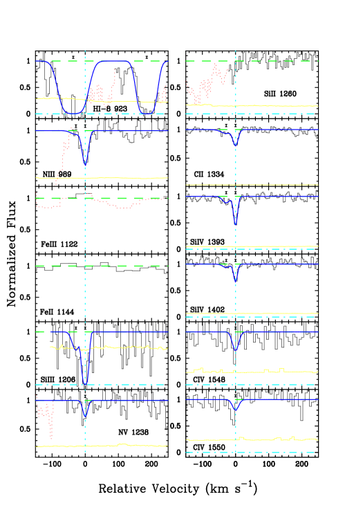
Figure 3.— Metal-line profiles for the LL system at $z=1.92$. Overplotted are our fits to the absorption profiles derived with the VPFIT software package. For completeness, we include all metal-line transitions where one might expect to observe an absorption profile. We indicate regions of the profiles contaminated by other absorption lines by dotting the data. The error array is the light gray line.

4.1. z=1.92

This QAL system has a total HI column density ${N({\rm HI})}=10^{17.15}\,{\rm cm^{-2}}$ and is responsible for the Lyman limit at $\approx 2700$ Å. It exhibits a number of metal-line transitions commonly observed in LL systems (presented in Figure 3). To determine the ionic column densities from the absorption line profiles, we have utilized the VPFIT software package in a manner similar to that for the ${N({\rm HI})}$ determinations. When fitting the profiles we introduced the minimum number of components necessary to yield a statistically ’good’ fit. The profiles trace one another very closely in velocity space such that we successfully tied the redshifts and Doppler parameter of each component for all of the ions. This point has significant bearing on our analysis because we believe the correspondence indicates all of the ions are spatially coincident and can be treated together in a single photoionization calculation. Furthermore, it implies there is little variation in the ionization state along the sightline. The VPFIT solutions and $1\sigma$ errors are presented in Table 3. With only a few exceptions, the solutions very closely match the results from Outram et al. (1998). We have also checked the ionic column density measurements by applying the Apparent Optical Depth Method (Savage and Sembach (1991)) which shows excellent agreement. For those transitions which exhibit no significant absorption, we report $3\sigma$ upper limits to their ionic column densities.

Table 3

Ionic Column Densities for the $z$=1.92 System Comp $z$ $\sigma_{z}$ b $\sigma_{b}$ Ion log $N$ $\sigma_{\rm{log}{\it N}}$ $10^{-6}$ km/s km/s $\,{\rm cm^{-2}}$ $\,{\rm cm^{-2}}$ 1 1.925970 3 6.13 0.41 Si⁺³ 12.78 0.02 6.13 Si⁺⁺ 13.84 0.78 9.37 C⁺ 13.12 0.03 9.37 C⁺³ 13.12 0.14 8.68 N⁺⁺ 13.79 0.12 8.68 N⁺⁴ 13.06 0.15 2 1.925695 14 13.89 3.00 Si⁺³ 12.25 0.08 13.89 Si⁺⁺ 12.32 0.38 21.24 C⁺ 12.78 0.10 19.67 N⁺⁺ 12.93 0.62 Fe⁺ $<13.3$ Fe⁺⁺ $<13.5$

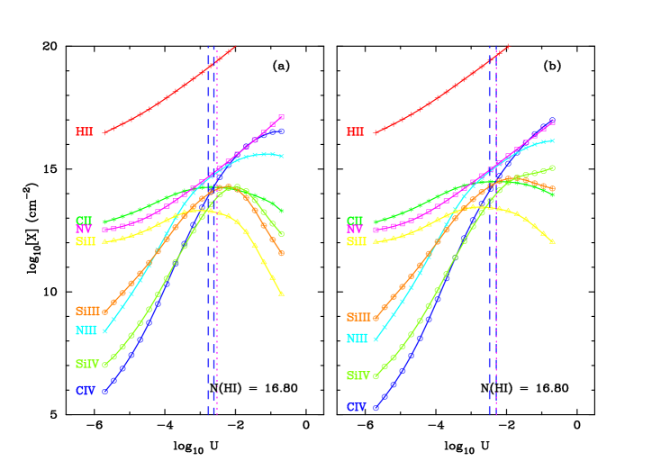
Figure 4.— The results from a series of CLOUDY calculations (Ferland 1995) assuming $\log{N({\rm HI})}=16.8$ with (a) a Haardt-Madau ionizing spectrum and (b) the Valls-Gabaud/Vernet model. Plotted are the calculated mean ionic column densities (assuming intrinsic solar abundances and [Fe/H] = $-0.5$) versus a modified ionization parameter, $U$, as defined in the text. The vertical dashed lines indicate the observed C⁺/C⁺³ ratio (with errors) and the dotted vertical line is a lower limit to $U$ determined from the upper limit to the Si⁺/Si⁺³ ratio.

The fact that the HI gas is distributed between two main components complicates the analysis. Examining Figure 3, one notes that the metal-line profiles lie near the blue HI component ($z=1.9256$), albeit not strictly at the center of the profile (compare with the absorption profiles for the $z=1.94$ system). Furthermore, we observe no significant metal-line profile for the HI component at $z=1.9278$. It is very possible that the LL system is actually comprised of two spatially separated absorbers with a velocity separation of $\approx 200{\rm\;km\;s^{-1}}$ along the sightline. Because we cannot constrain the geometry of these absorbers, our CLOUDY simulations are an oversimplification. In the following, we treat the absorbers separately and focus on the HI component at $z=1.9256$ with ${N({\rm HI})}=10^{16.79}\,{\rm cm^{-2}}$ which corresponds to the metal-line profiles. Finally, we will use the results of our analysis to place limits on the metallicity of the other HI component. While it is possible that the $z=1.9278$ absorber may attenuate the EUVB radiation, we find that the ionization corrections hardly vary for $\log{N({\rm HI})}=16.8-17.2\,{\rm cm^{-2}}$ and therefore do not consider shielding to be a problem.

Table 4

Chemical Abundances for the z=1.92 System Ion Haardt/Madau Valls-Gabaud/Vernet [X/H] [X/H] C⁺ $-1.47\pm 0.1$ $-1.70\pm 0.1$ C⁺³ $-1.47\pm 0.2$ $-1.70\pm 0.2$ N⁺⁺ $-1.35\pm 0.2$ $-1.66\pm 0.2$ N⁺⁴ $-2.28\pm 0.3$ $-2.57\pm 0.3$ Si⁺ $<-1.54$ $<-1.68$ Si⁺³ $-1.16\pm 0.15$ $-1.43\pm 0.15$ Fe⁺ $<1.6$ $<1.5$ Fe⁺⁺ $<-0.1$ $<-0.2$

Given the ionic column densities and our measurement of ${N({\rm HI})}$, we can constrain the ionization state of this system by comparing the relative ionic column densities with the calculations from the CLOUDY package. To eliminate the effects of the underlying abundance pattern (e.g. Type II SN enhancements) and dust depletion, we will focus on multiple ions from a single element. For this LL system, the tightest constraints are imposed by the C⁺/C⁺³ ratio. Figure 4 presents the CLOUDY solutions (calculated ionic column densities) for a plane-parallel slab with ${N({\rm HI})}=10^{16.8}\,{\rm cm^{-2}}$ photoionized by (a) an HM EUVB spectrum and (b) the VV spectrum for a range of ionization parameter assuming [Fe/H]=$-0.5$ dex. The results are largely independent of the metallicity assumed in the CLOUDY calculation; varying [Fe/H] uniformly varies all of the predicted column densities. The dashed vertical lines indicate the $U$ values corresponding to $\log[{N({\rm CII})}/{N({\rm CIV})}]=0.16\pm 0.2$ while the dotted line denotes a lower limit to $U$ derived from $\log[{N({\rm SiII})}/{N({\rm SiIV})}]<-0.66$. For the HM spectrum, the C⁺/C⁺³ and Si⁺/Si⁺³ ratios are consistent at the $2\sigma$ level and indicate $\log U=-2.69\pm 0.1$ and ${N({\rm H})}=19.21\pm 0.20$ dex. This implies $n_{H}=1{\rm\;\times\;10^{-2}}\,{\rm cm^{-3}}\,(J_{912}/10^{-21.5})$ which agrees with limits to $n_{H}$ in other LL systems (Steidel (1990); Prochaska (1999)). In terms of the VV EUVB model, the results are comparable with a slightly higher prediction for ${N({\rm H})}$ and $U$: $\log U=-2.38\pm 0.1$, ${N({\rm H})}=19.51\pm 0.2$ dex, and $n_{H}=5{\rm\;\times\;10^{-3}}\,{\rm cm^{-3}}\,(J_{912}/10^{-21.5})$. Ignoring the effects of clumping within the LL system, this implies a characteristic length scale, $\ell\sim{N({\rm H})}/n_{H}\sim 1$ kpc.

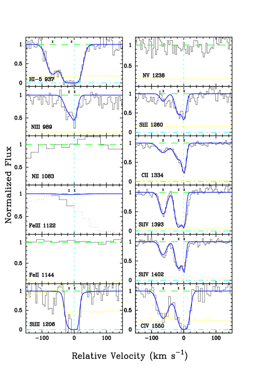
Figure 5.— Metal-line profiles for the QAL system at $z=1.94$. Overplotted are our fits to the absorption profiles derived with the VPFIT software package. For completeness, we include all metal-line transitions where one might expect to observe an absorption profile. We indicate regions of the profiles contaminated by other absorption lines by dotting the data. The error array is the light gray line.

Having placed relatively tight constraints on the ionization state, we can calculate the chemical abundances for this system by making ionization corrections to the observed ionic column densities. Table 4 lists the abundances relative to solar ([X/H] $\equiv$ ${\rm\log[{N({\rm X})}/{N({\rm H})}]-\log[X/H]_{\odot}}$) derived from each ion for the two EUVB models. The error bars account for uncertainties in ${N({\rm HI})}$, $U$, and the ionic column density. Note the very small error to the [C/H] value derived from ${N({\rm CII})}$. As one observes from Figure 4, the relevant $U$ values span a very flat section of the CII curve such that [C/H] is nearly independent of $U$. Therefore, the Carbon abundance has a very small error to its ionization correction, i.e., the error in [C/H] is dominated by the uncertainty in the ${N({\rm HI})}$ measurement. This implies CII measurements can provide reasonably robust metallicity measurements for all LL systems with ${N({\rm HI})}\approx 10^{17}\,{\rm cm^{-2}}$. For this system, we find [C/H] = $-1.47\pm 0.1$ dex for the HM spectrum and [C/H] = $-1.70\pm 0.1$ dex adopting the VV model. The values are typical of other estimates for Lyman limit systems at high $z$ (Steidel (1990); Burles & Tytler (1998)). Comparing the Silicon abundance ([Si/H] = $-1.16\pm 0.15$ for HM and [Si/H] = $-1.43\pm 0.15$ for the VV model) derived from ${N({\rm SiIV})}$ against [C/H] we observe good agreement which gives further confidence in our modeling as the values are independent of the C and Si ionic ratios. The relative abundance of C to Si, [C/Si] = $-0.3\pm 0.1$ dex, is consistent with solar abundances at the $3\sigma$ level, but favors the ratio of $-0.3$ dex observed in Population II stars as expected for low metallicity systems. In all, we confidently report that the HI component at $z=1.9256$ has a metallicity of $\approx 1/50$ solar abundance. Without any ionic column density measurements with which to constrain the ionization state of the HI component at $z=1.9278$, one can only speculate on its metallicity. Assuming that the ionization state matches that of the blue HI component, we find [C/H]$<-2.4$ dex from a $3\sigma$ upper limit to the CII $\lambda 1334$ column density.

4.2. z=1.94

From an examination of a low resolution spectrum of J2233$-$606, Sealey et al. (1998) proposed this QAL system is responsible for the Lyman limit system observed at $\approx 2700$ Å. Figure 2 clearly demonstrates, however, that the Lyman series is not saturated at Ly-10 and therefore the system is optically thin at the Lyman limit. In Figure 5 we present the velocity profiles of the metal-line transitions overplotted by the VPFIT solution (Table 5) for those transitions where an unblended absorption feature is present. As with the Lyman limit system at $z=1.92$, the low ionization states (e.g. C⁺, Si⁺) very accurately trace the high-ion profiles. Therefore, we fit all of the profiles by tying the redshifts and Doppler parameters of the individual components. Unlike the system at $z=1.92$, the metal-lines also closely trace the HI gas and we treat all of the gas as a single system.

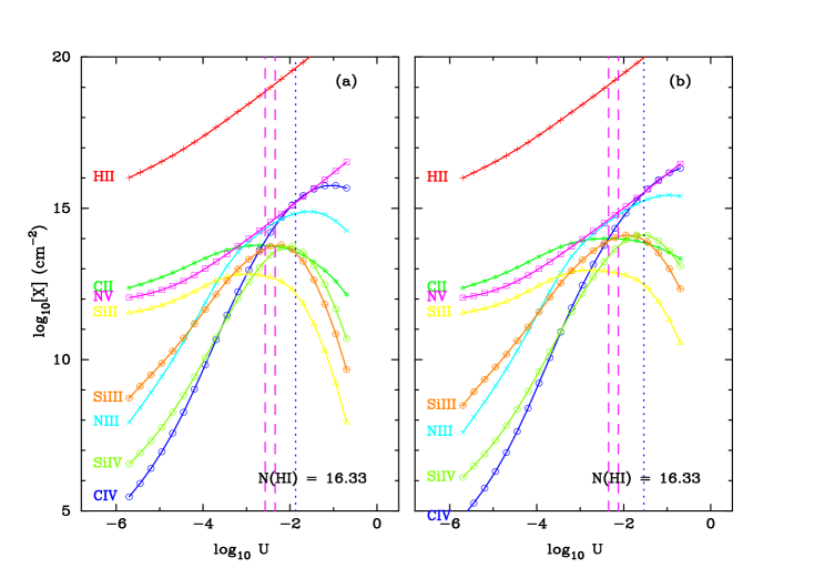
Figure 6.— The results from a series of CLOUDY calculations (Ferland 1995) assuming $\log{N({\rm HI})}=16.33$ with (a) a Haardt-Madau ionizing spectrum and (b) the Valls-Gabaud/Vernet model. Plotted are the calculated mean ionic column densities (assuming intrinsic solar abundances and [Fe/H] = $-0.5$) versus a modified ionization parameter, $U$, as defined in the text. The vertical dotted lines indicate the observed Si⁺/Si⁺³ ratio (with errors) and the dotted vertical line is a very rough estimate to $U$ from the C⁺/C⁺³ ratio.

Table 5

Ionic Column Densities for the $z$=1.94 System Comp $z$ $\sigma_{z}$ b $\sigma_{b}$ Ion log $N$ $\sigma_{\rm{log}{\it N}}$ $10^{-6}$ km/s km/s $\,{\rm cm^{-2}}$ $\,{\rm cm^{-2}}$ 1 1.942614 4 6.17 0.44 Si⁺ 12.69 0.12 6.17 Si⁺⁺ 15.03 0.81 6.17 Si⁺³ 13.32 0.06 9.44 C⁺ 13.63 0.04 9.21 C⁺³ 15.35 0.56 8.74 N⁺⁺ 13.67 0.18 2 1.942441 10 11.11 0.83 Si⁺ 12.71 0.10 11.11 Si⁺⁺ 13.06 0.43 11.11 Si⁺³ 13.44 0.04 17.00 C⁺ 13.56 0.05 17.00 C⁺³ 13.80 0.27 15.76 N⁺⁺ 13.71 0.14 3 1.941976 5 11.26 0.53 Si⁺ 12.15 0.20 11.26 Si⁺³ 13.03 0.03 17.22 C⁺ 13.26 0.03 17.22 C⁺³ 14.04 0.14 N⁺⁴ $<13.3$ Fe⁺ $<13.1$ Fe⁺⁺ $<13.1$

Figure 6 presents the CLOUDY calculations for a QAL absorption line system with ${N({\rm HI})}=10^{16.33}\,{\rm cm^{-2}}$ and [Fe/H] = $-0.5$ dex adopting (a) a HM EUVB spectrum and (b) the VV EUVB model. Since this system is optically thin at the Lyman limit, the results are largely insensitive to the ${N({\rm HI})}$ value. Similar to our examination of the $z=1.92$ system, we overplot the allowed values for the ionization parameter given the observed ionic ratios for Si⁺/Si⁺³ and C⁺/C⁺³. Because the SiIII and CIV profiles are heavily saturated, the most significant constraints for the ionization state are from the Si⁺/Si⁺³ ratio, ${N({\rm SiII})}/{N({\rm SiIV})}=-0.70\pm 0.15$ dex. For the HM spectrum, we find $\log U=-2.46\pm 0.1$ which implies $\log{N({\rm H})}=18.98\pm 0.15\,{\rm cm^{-2}}$ and $n_{H}\approx 6{\rm\;\times\;10^{-3}}\,{\rm cm^{-3}}\,(J_{912}/10^{-21.5})$. Meanwhile, comparing against the CLOUDY solution for the VV EUVB spectrum, the values are: $\log U=-2.24\pm 0.1$, $\log{N({\rm H})}=19.19\pm 0.2\,{\rm cm^{-2}}$, and $n_{H}\approx 6{\rm\;\times\;10^{-3}}\,{\rm cm^{-3}}\,(J_{912}/10^{-21.5})$.

Table 6 lists the abundances relative to solar for this system for the two EUVB models. The variance in the ionization corrections for Si⁺ and C⁺ are very small ($<0.1$ dex) so it is very reassuring that the derived [C/H] and [Si/H] values are in good agreement: [C/H] = $-0.27\pm 0.1$ (HM), [C/H] = $-0.50\pm 0.1$ (VV) and [Si/H = $-0.14\pm 0.1$ (HM), [Si/H] = $-0.31\pm 0.1$ (VV). Altogether, the system has a relatively large metallicity, $\approx{1\over 2}-{1\over 3}$ solar metallicity. This value is even larger than what is typically observed for the damped Ly$\alpha$ systems at $z\approx 2$ (Pettini et al. (1997); Prochaska & Wolfe (1999)). In $\S$ 4 we will discuss the implications of this result.

Table 6

Chemical Abundances for the Z=1.94 System Ion Haardt/Madau Valls-Gabaud/Vernet [X/H] [X/H] C⁺ $-0.27\pm 0.1$ $-0.50\pm 0.1$ C⁺³ $-0.06\pm 0.6$ $-0.15\pm 0.6$ N⁺⁺ $-0.93\pm 0.2$ $-1.17\pm 0.2$ N⁺⁴ $<-3.00$ $<-3.15$ Si⁺ $-0.14\pm 0.1$ $-0.31\pm 0.1$ Si⁺³ $-0.14\pm 0.1$ $-0.31\pm 0.15$

4.3. HIGHER IONIZATION GAS

We have also considered constraints on the ionization state for each system placed by a lower limit to the N⁺⁺/N⁺⁴ ratio. The Nitrogen ratios are inconsistent with both EUVB models for all values of $U$ in each system. We expect this disagreement arises because of a mistreatment of N⁺⁴. N⁺⁴ is the only ion we examined with an ionization potential greater than 4 Ryd and is therefore the most sensitive to three factors: (1) the shape of the EUVB spectrum at $h\nu>4$ Ryd, (2) the optical depth of HeII in the IGM, and (3) the optical depth of HeII within the metal-line system. Because the number density of quasars peaks near $z=2$, it is unlikely that the EUVB spectrum is significantly softer than the VV model which does account for a contribution from background galaxies. Regarding the second point, the optical depth of HeII in the IGM is measured to be quite small at $z=2.4$ ($\tau_{HeII}=1.0\pm 0.07$; Davidsen et al. (1996)) and is expected to be significantly lower at $z\approx 2$. Therefore, we expect the high N⁺⁺/N⁺⁴ ratio implies an oversimplification in modeling HeII within the CLOUDY framework. Whereas the CLOUDY package assumes the metals are uniformly dispersed throughout the absorption-line system, it is quite possible the metals are primarily located in the central regions where they could be shielded from high energy photons by the surrounding He gas. For both systems, one predicts ${N({\rm HeII})}>10^{17.8}\,{\rm cm^{-2}}$ which imply an optical depth $\tau_{HeII}>1$ that is more than enough to account for the $\approx 0.3$ dex discrepancy between the observations and CLOUDY predictions. Unfortunately, this means one cannot use the NIII or NV absorption profiles for constraining the ionization state or abundances of this system. At the same time, however, it is important to stress that these issues have little effect on the ionization fractions of C and Si as they are largely insensitive to the flux of photons with energies $>4$ Ryd.

5. SPECULATIONS AND FUTURE OBSERVATIONS

The similarities and differences observed for the two metal-line systems toward J2233$-$606 are compelling. The systems differ by only $\approx 0.6$ dex in ${N({\rm HI})}$ and have comparable total Hydrogen column densities. The inferred $n_{H}$ and ionization fractions are also in good agreement. Furthermore, the kinematic characteristics of the metal-line profiles closely resemble one another. The profiles are relatively narrow ($<100{\rm\;km\;s^{-1}}$ in velocity space) and exhibit only a modest asymmetry. One might expect, therefore, that while the $z=1.94$ system may have a slightly lower ${N({\rm H})}$ value, the two systems have a similar physical origin. There is, however, a significant division between the two systems; the $z=1.94$ system has a metallicity over 20 times larger than the $z=1.92$ system. We believe this striking comparison belies a fundamental difference in the physical nature of the two systems.

To date, several models for the physical nature of the Lyman limit systems have been proposed. Several groups have demonstrated that a significant fraction of $z\approx 1$ LL systems are associated with the outer regions (e.g. halos) of $\approx$ L^∗ galaxies (Bergeron & Boiss$\rm\grave{e}$ (1991); Steidel & Dickinson (1992)). This suggests that at $z\approx 2$ one expects the Lyman limit systems to be associated with galactic or protogalactic systems. On the other hand, numerical hydrodynamic simulations (Katz et al. (1996)) indicate that LL systems may also arise in the large scale structure (LSS; e.g. filaments, walls) of the Universe. The $z=1.92$ system, with its low metallicity, is a candidate for both of these models. If the system is associated with a galaxy, then either very little star formation (e.g. a dwarf galaxy) has taken place or the sightline intersects gas in the unenriched outer parts of the galaxy. Also, the observation of two significant HI components would indicate substructure within a single galaxy, or perhaps that the sightline actually intersects two galaxies. The fact that the metal-line profiles do not exactly coincide with either HI component, however, may be difficult to reconcile in terms of a galactic system where one might expect the HI gas to exactly trace the CII gas. At the same time, the observations can be explained within the framework of a LSS origin. This scenario, similar to the description of the Ly$\alpha$ forest within N-body simulations, links the Lyman limit system with an unvirialized LSS in the universe, e.g., a filament. The metallicity is sufficiently small that the metals could have been injected at much earlier time by a galactic system as is proposed for the enrichment of the Ly$\alpha$ forest (Tytler et al. (1995); Cowie & Songaila (1998); Lu et al. (1998)). The significant difference in the metallicity for the two HI components, however, argues for a local production of the metals (e.g. a hydrodynamic shock in the LSS). While it is not difficult to envision a LSS scenario which explains the two HI components and the misalignment of the metal-line profiles, more research on this topic is necessary to reveal the likelihood of these observations. Perhaps one will find it is a general prediction from the numerical simulations that one would not expect the HI gas to directly align with the metal-line profiles.

In contrast, the high metallicity of the $z=1.94$ system argues strongly against a LSS origin as it almost certainly requires the presence of a significant star forming region. Because the system is within 30,000 km s^-1 of the QSO, one must consider the possibility that it is an associated system. The fact that Ly-5 and the CIV profiles are fully saturated indicates no partial covering and argues strongly against this interpretation. Furthermore, no NV absorption is evident as would be expected for an associated system. Therefore, we contend the absorber at $z=1.94$ arises within a galactic system. In this scenario, the low ${N({\rm H})}$ and ${N({\rm HI})}$ values indicate that the sightline has a large impact parameter. In fact, unless the system is the result of a very compact star forming region, we predict one will identify it with the STIS imaging and follow-up observations. If the responsible galaxy is identified, than our analysis affords a direct measurement of the physical properties of a $z\approx 2$ galaxy.

By comparing our analysis with an examination of the imaging observations, one is able to investigate the the ISM in $z\approx 2$ galaxies (or in the case that no galaxy is identified, perhaps the properties of LSS). Unfortunately, one cannot rely on photometric redshifts to distinguish between $z=1.92$ and $z=1.94$, thus follow-up spectroscopy of all candidate galaxies will be essential. At the time of writing, we are aware of only one spectroscopic study (Tresse et al. (1998)) of the STIS field. While their observations identified no galaxies at $z\approx 1.9$, the observations were limited to I$<21$.

References

- Bergeron & Boiss (1991) Bergeron, J. & Boiss, P. 1991, A&A, 243, 344
- Boyle (1997) Boyle, B.J. 1997, AAO Newsletter, 83, 4
- Burles & Tytler (1998) Burles, S. and Tytler, D. 1998, ApJ, 507, 732
- Cowie & Songaila (1998) Cowie, L. L. & Songaila, A. 1998, Nature, 394, 44
- Davidsen et al. (1996) Davidsen, A. F., Kriss, G. A., & Zheng, W. 1996, Nature, 380, 47
- Ferguson et al. (1999) Ferguson, H.C. et al. 1999, AJ, submitted
- Ferland (1995) Ferland, G. J. 1995, Hazy, a Brief Introduction to Cloudy, Univ. Kentucky, Phys. Dept. Int. Rep
- Gardner et al. (1999) Gardner, J.P. et al. 1999, AJ, submitted
- Haardt & Madau (1996) Haardt, F. & Madau, P. 1996, ApJ, 461, 20
- Hamman & Ferland (1992) Hamman, F. & Ferland, G. 1992, ApJ, 391, L53
- Katz et al. (1996) Katz, N., Weinberg, D.H., Hernquist, L., Miralda-Escud, J. 1996, ApJ, 456, L57
- Lu et al. (1996) Lu, L., Sargent, W.L.W., Barlow, T.A., Churchill, C.W., & Vogt, S. 1996, ApJS, 107, 475
- Lu et al. (1998) Lu, L., Sargent, W. L. W., Barlow, T. A. & Rauch, M. 1998, submitted to AJ
- Outram et al. (1998) Outram, P.J., Boyle, B.J., Carswell, R.F., Hewett, P.C., Williams, R.E., & Norris, R.P. 1998, MNRAS, submitted
- Pettini et al. (1997) Pettini, M., Smith, L.J., King, D.L., & Hunstead, R.W. 1997, ApJ, 486, 665
- Prochaska (1999) Prochaska, J.X. 1999, ApJ, in press, astro-ph/9811357
- (17) Prochaska, J. X. & Wolfe, A. M. 1997, ApJ, 486, 73
- Prochaska & Wolfe (1998) Prochaska, J.X. & Wolfe, A.M. 1998, ApJ, 507, 113
- Prochaska & Wolfe (1999) Prochaska, J.X. & Wolfe, A.M., 1999, ApJ, in press, astro-ph/9810301
- Savage and Sembach (1991) Savage, B. D. and Sembach, K. R. 1991, ApJ, 379, 245
- Savaglio (1998) Savaglio, S. 1998, preprint
- Sealey et al. (1998) Sealey, K.M., Drinkwater, M.J., & Webb, J.K. 1998, ApJ, submitted, astro-ph/9804018
- Steidel (1990) Steidel, C.C. 1990, ApJS, 74, 37
- Steidel & Dickinson (1992) Steidel, C.C. & Dickinson, M. 1992, ApJ, 394, 81
- Tresse et al. (1998) Tresse, L., Dennefeld, M., Petitjean, P., Cristiani, S., & White, S. 1998, A&A, submitted, (astro-ph/9812246)
- Tytler et al. (1995) Tytler, D., Fan, X.-M., Burles, S., Cottrell, L., Davis, C., Kirkman, D., & Zuo, L. 1995, in QSO Absorption Lines, ed. G. Meylan (Springer-Verlag), 289
- Valls-Gabaud & Vernet (1999) Valls-Gabaud, D. & Vernet J., MNRAS, in preparation
- Williams et al. (1999) Williams, R. et al. 1999, AJ, submitted