POTENT RECONSTRUCTION FROM MARK III VELOCITIES

Abstract

We present an improved version of the POTENT method for reconstructing the velocity and mass density fields from radial peculiar velocities, test it with mock catalogs, and apply it to the Mark III Catalog of Galaxy Peculiar Velocities. The method is improved in several ways: (a) the inhomogeneous Malmquist bias is reduced by grouping and corrected statistically in either forward or inverse analyses of inferred distances, (b) the smoothing into a radial velocity field is optimized such that window and sampling biases are reduced, (c) the density field is derived from the velocity field using an improved weakly non-linear approximation in Eulerian space, and (d) the computational errors are made negligible compared to the other errors. The method is carefully tested and optimized using realistic mock catalogs based on an N-body simulation that mimics our cosmological neighborhood, and the remaining systematic and random errors are evaluated quantitatively.

The Mark III catalog, with $\sim\!3300$ grouped galaxies, allows a reliable reconstruction with fixed Gaussian smoothing of $10-12\,h^{-1}{\rm Mpc}$ out to $\sim\!60\,h^{-1}{\rm Mpc}$ and beyond in some directions. We present maps of the three-dimensional velocity and mass-density fields and the corresponding errors. The typical systematic and random errors in the density fluctuations inside $40\,h^{-1}{\rm Mpc}$ are $\pm 0.13$ and $\pm 0.18$. The recovered mass distribution resembles in its gross features the galaxy distribution in redshift surveys and the mass distribution in a similar POTENT analysis of a complementary velocity catalog (SFI), including the Great Attractor, Perseus-Pisces, and the large void in between. The reconstruction inside $\sim 40\,h^{-1}{\rm Mpc}$ is not affected much by a revised calibration of the distance indicators (VM2, tailored to match the velocities from the IRAS 1.2 Jy redshift survey). The bulk velocity within the sphere of radius $50\,h^{-1}{\rm Mpc}$ about the Local Group is $V_{\rm 50}=370\pm 110\,{\rm km}\,{\rm s}^{-1}$ (including systematic errors), and is shown to be mostly generated by external mass fluctuations. With the VM2 calibration, $V_{\rm 50}$ is reduced to $305\pm 110\,{\rm km}\,{\rm s}^{-1}$.

1 INTRODUCTION

The development of methods for estimating distances to galaxies independently of their redshifts enables direct, quantitative study of large-scale dynamics (reviews: Dekel 1994; Strauss & Willick 1995; Willick 1998; Dekel 1998a). The inferred peculiar velocities of thousands of galaxies are interpreted as noisy tracers of an underlying peculiar velocity field. Under the assumption of structure evolution via gravitational instability (GI), one can recover the velocity-potential field and the associated fields of three-dimensional velocity and mass-density fluctuations. These dynamical fields have important theoretical implications. For example, they are related directly to the initial fluctuations on scales ranging from $\sim\!10$ to $\sim\!100\,h^{-1}{\rm Mpc}$, independent of galaxy-density “biasing”, and they provide unique constraints on the value of the cosmological density parameter, $\Omega$. Combined with galaxy redshift surveys, the dynamical fields can be used to address the “biasing” relation between galaxies and mass and help us better understand galaxy formation. When compared to the fluctuations in the Cosmic Microwave Background (CMB), they allow a unique test of GI as the source for fluctuation growth, and they provide constraints on the fluctuation power spectrum on intermediate scales.

There is growing evidence in support of the hypothesis that the inferred large-scale peculiar velocity field is real, and of gravitational origin. First, the $\delta T/T\sim 10^{-5}$ temperature fluctuations detected in the CMB are consistent with gravity’s generating $\sim 300$-$400\,{\rm km}\,{\rm s}^{-1}$ flows across regions of size $\sim 100\,h^{-1}{\rm Mpc}$, as inferred from the observed peculiar velocities (e.g., Bertschinger, Gorski & Dekel 1990). Second, the velocity fields inferred independently from spiral and from elliptical galaxies, using different distance indicators, are consistent with being noisy versions of the same underlying velocity field (Kolatt & Dekel 1994; re-confirmed for the Mark III data, unpublished; Scodeggio 1997). Third, the gross features of the galaxy density field from redshift surveys are similar, within the errors, to the features of the mass-density field derived under GI from the observed peculiar velocities (Dekel et al. 1993; Hudson et al. 1995; Sigad et al. 1998), ruling out in particular certain alternative models in which the galaxy distribution could violate the continuity equation (Babul et al. 1994).

The important implications of the dynamical fields, and the encouraging evidence for their reality and gravitational origin, motivate an effort of analysis within the framework of GI. This is the aim of the POTENT program and related investigations. Bertschinger and Dekel (1989, BD) proposed the original idea to recover the three-dimensional velocity field using the expected irrotationality of gravitational flows in the weakly non-linear regime, and demonstrated the feasibility of such a method. A first version of the method was developed and tested by Dekel, Bertschinger & Faber (1990, DBF), and first maps of the recovered fields in our near cosmological neighborhood were presented, based on the Mark II data that were available at that time (Bertschinger, Dekel, Faber, Dressler & Burstein 1990, BDFDB). The present paper is the main paper of the second-generation POTENT analysis, describing and evaluating in detail the improved method and presenting maps and simple statistics based on the extended Mark III data (Willick et al. 1997a).

The aim of the POTENT analysis is to recover with minimal systematic errors the velocity and density fields that would be obtained if the true three-dimensional velocity field were sampled uniformly and with infinite density, and smoothed with a spherical Gaussian window of a fixed radius (hereafter G$R_{\rm s}$, where $R_{\rm s}$ is the smoothing radius in $\!\,h^{-1}{\rm Mpc}$, e.g., G10, G12, etc.). The spatial statistical uniformity implied by the fixed smoothing scale, which is a special feature of POTENT, is useful both for pure cosmographic purposes and for simple, direct comparisons of the recovered fields with theoretical models and other observations. Note that, for certain specific purposes, such as a velocity-velocity comparison with a redshift survey for determining the parameter $\beta$ ($\equiv\Omega^{0.6}/b$, where $b$ is the relevant biasing parameter), one also has the option of applying variable  smoothing that can be optimized to match the non-uniform sampling and errors in the data. This is true in POTENT as well as in other methods (e.g., DBF; BDFDB; Davis, Nusser & Willick 1996, ITF; Willick et al. 1997b, VELMOD). For example, a reconstruction method using a Wiener filter for a rigorous treatment of the random errors (Zaroubi, Hoffman & Dekel 1998) naturally applies such a variable smoothing that is determined by the data, noise and a prior power spectrum. The Wiener fields are then forced to a fixed smoothing by generating constrained realizations.

A few more introductory words about the key idea of POTENT are in order for the reader who is not familiar with DBF. If the large-scale structure evolved according to GI, the large-scale peculiar velocity field is expected to be irrotational, $\kern-0.24994pt\hbox{$\nabla$}\kern-8.33336pt\kern 0.50003pt\hbox{$\nabla$}\kern-8.33336pt\kern-0.24994pt\raise 0.43304pt\hbox{$\nabla$}\!\times\!\kern-0.24994pt\hbox{$v$}\kern-5.20601pt\kern 0.50003pt\hbox{$v$}\kern-5.20601pt\kern-0.24994pt\raise 0.43304pt\hbox{$v$}=0$. Any vorticity mode would have decayed away during the linear phase of fluctuation growth as the universe expanded, and, based on Kelvin’s circulation theorem, the flow remains vorticity-free in the weakly non-linear regime as long as it is laminar, i.e., with no orbit crossing (DBF). This has been shown to be a good approximation when collapsed regions are properly smoothed over, on scales of a few Mpc or more (DB; DBF). Irrotationality implies that the velocity field can be derived from a scalar potential, $\kern-0.24994pt\hbox{$v$}\kern-5.20601pt\kern 0.50003pt\hbox{$v$}\kern-5.20601pt\kern-0.24994pt\raise 0.43304pt\hbox{$v$}(\kern-0.24994pt\hbox{$x$}\kern-5.71527pt\kern 0.50003pt\hbox{$x$}\kern-5.71527pt\kern-0.24994pt\raise 0.43304pt\hbox{$x$})\!=\!-\kern-0.24994pt\hbox{$\nabla$}\kern-8.33336pt\kern 0.50003pt\hbox{$\nabla$}\kern-8.33336pt\kern-0.24994pt\raise 0.43304pt\hbox{$\nabla$}\Phi(\kern-0.24994pt\hbox{$x$}\kern-5.71527pt\kern 0.50003pt\hbox{$x$}\kern-5.71527pt\kern-0.24994pt\raise 0.43304pt\hbox{$x$})$, and thus the radial velocity field $u(\kern-0.24994pt\hbox{$x$}\kern-5.71527pt\kern 0.50003pt\hbox{$x$}\kern-5.71527pt\kern-0.24994pt\raise 0.43304pt\hbox{$x$})$, which also consists of one number at each point in space, should contain enough information for a full reconstruction. In the standard POTENT procedure, the velocity potential is computed by integration along radial rays from the observer,

$$\Phi(\kern-0.24994pt\hbox{$x$}\kern-5.71527pt\kern 0.50003pt\hbox{$x$}\kern-5.71527pt\kern-0.24994pt\raise 0.43304pt\hbox{$x$})=-\int_{0}^{r}u(r^{\prime},\theta,\phi)dr^{\prime}\ .$$ (1)

The two missing transverse velocity components along $\theta$ and $\phi$ are then recovered by differentiation, and the underlying mass-density fluctuation field is computed from the partial derivatives of the velocity field using a mildly non-linear approximation (see § 5).

The POTENT procedure thus recovers the underlying mass-density fluctuation field from a whole-sky sample of observed radial peculiar velocities via the following steps:

• Prepare the radial velocities for POTENT analysis, in particular correcting for Malmquist bias in different ways, including grouping.

• Smooth the peculiar velocities into a uniformly-smoothed radial velocity field that has minimum bias.

• Apply the ansatz of gravitating potential flow to recover the potential and three-dimensional velocity field.

• Derive the underlying mass density field by an approximation to GI in the mildly non-linear regime.

• Evaluate the remaining systematic and random errors using mock catalogs.

The most challenging part of the POTENT procedure is the second step in the above list, where one tries to obtain an unbiased radial-velocity field $u(\kern-0.24994pt\hbox{$x$}\kern-5.71527pt\kern 0.50003pt\hbox{$x$}\kern-5.71527pt\kern-0.24994pt\raise 0.43304pt\hbox{$x$})$ from the observed noisy and sparsely sampled radial velocities of galaxies (§ 6).

The present analysis is superior to the original POTENT analysis of 1990 in several ways:

• The new Mark III catalog contains $\sim 3300$ galaxies, mostly spirals with $\sim\!17\!-\!21\%$ distance errors, compared with only $\sim\!970$ galaxies in Mark II, which were dominated by ellipticals with 21% errors. The Mark III catalog samples with higher resolution an extended volume of typical radius $\sim\!60\!-\!70\,h^{-1}{\rm Mpc}$ about the Local Group (LG). This catalog, assembled from several different datasets, is carefully calibrated and merged into a self-consistent sample (§ 2).

• New efforts have been made to minimize systematic errors in the data, such as Malmquist bias (§ 7).

• The derivation of the smoothed radial velocity field from the discrete peculiar velocities is better designed and tested to minimize systematic errors due to the tensor window imposed by the radial velocities and due to the sparse and non-uniform sampling (§ 6).

• The potential analysis is done with higher resolution and improved accuracy such that the computational errors become negligible compared to the other uncertainties (§ 5).

• The density field, which in DBF involved an elaborate iterative procedure in Lagrangian space, is now recovered from the velocity field using a straightforward Eulerian prescription (§ 5).

This paper is organized as follows. In § 2 we briefly describe the Mark III data. In the following six sections we describe the POTENT method and its testing step by step using mock catalogs. In § 3 we describe the mock catalogs that serve as our major tool for evaluating errors. In § 4 we define the statistics to be used in the evaluation of the reconstruction. In § 5 we elaborate on the potential analysis and the derivation of the density field. In § 6 we discuss in detail the smoothing procedure and the minimization of the associated systematic errors. In § 7 we describe three different schemes for correcting Malmquist bias. In § 8 we define our reference volumes and evaluate the remaining errors in the POTENT analysis within these volumes.

The next two sections describe the results of applying POTENT to the actual Mark III catalog: in § 9 we present maps of velocity and mass-density fields and in § 10 we compute the bulk velocity in spheres and shells about the Local Group and show preliminary results concerning a decomposition of the velocity field into its divergent and tidal components.

Finally, in § 11, we discuss issues concerning the method and the data, summarize the cosmological implications and comment on alternative methods and other results. We conclude with a summary in § 12.

2 THE MARK III CATALOG

The Mark III Catalog of Galaxy Peculiar Velocities (Willick et al. 1995; 1996; 1997a) consists of roughly 3300 galaxies from several different datasets of spiral and elliptical/S0 galaxies. The distances were inferred by the Tully-Fisher (TF) and $D_{n}\!-\!\sigma$ distance indicators, respectively. These are based on empirical intrinsic linear correlations between a distance independent quantity (the log of the internal velocity in a galaxy, $\eta$, referring to rotation in spirals and dispersion in ellipticals) and a distance-dependent quantity (the apparent magnitude in spirals and the log of the apparent diameter in ellipticals). The “forward” TF relation between the intrinsic quantities $\eta$ and absolute magnitude $M$ is

$$M_{\scriptscriptstyle\rm TF}(\eta)=a-b\eta\ .$$ (2)

It yields an inferred distance $d$ from observed values of $\eta$ and apparent magnitude $m$ via the standard distance-modulus relation

$$5\log d=m-M_{\scriptscriptstyle\rm TF}(\eta)\ .$$ (3)

The CMB redshift $z$ of the galaxy is obtained from the helio-centric redshift using the standard transformation based on COBE’s 4-year dipole (Lineweaver et al. 1996), and the inferred radial peculiar velocity at $d$, in the CMB frame, is

$$u=z-d\ ,$$ (4)

where all quantities are measured in $\!\,{\rm km}\,{\rm s}^{-1}$, i.e., the speed of light $c$ and the Hubble constant $H_{0}$ are set to unity. [We measure distances equivalently by $\!\,{\rm km}\,{\rm s}^{-1}\,$ or by $\!\,h^{-1}{\rm Mpc}$, where $h\equiv H_{0}/(100\,{\rm km}\,{\rm s}^{-1}{\rm Mpc}^{-1})$.]

The slope of the TF relation, $b$, can be derived from cluster galaxies that are assumed to be at a common distance within each cluster. The TF zero point, $a$, which fixes the absolute distance scale (in $\,{\rm km}\,{\rm s}^{-1}$, or $\,h^{-1}{\rm Mpc}$, still independent of the actual value of the Hubble constant), is free to be determined by minimizing residuals about a Hubble flow in a volume as large as possible. The scatter about the mean TF relation is between $0.35$ and $0.45$ magnitudes, which translates to a random uncertainty of $17$-$21\%$ in the inferred distance.

The large-scale backbone of the Mark II data was the whole-sky set of $\sim\!500$ ellipticals and S0’s dominated by Lynden-Bell et al. (1988, known as the “7-Samurai” or “7S” survey), supplemented by data from Dressler & Faber (1991) and Lucey & Carter (1988). The more local neighborhood, out to $\sim 30\,h^{-1}{\rm Mpc}$, was dominated by a set of spirals, mostly from Aaronson et al. (1982; A82). In the Mark III catalog we have added the large southern sample of spirals by Mathewson, Ford & Buchhorn (1992; MAT), the northern sample by Courteau & Faber (Courteau 1996, 1997; CF), the narrow-angle sample towards Perseus-Pisces by Willick (1991; W91PP), and the whole-sky cluster sample by Han, Mould and collaborators (Han & Mould 1990, 1992; Mould et al. 1991; HMCL). We also revised the A82 data set based on the uniform diameters and related revisions by Tormen & Burstein (1995). The full catalog consists of $\sim\!2800$ spirals. Table 1 summarizes the main properties and selection criteria of the datasets that make up the Mark III catalog. The number of galaxies actually used from each dataset in the POTENT application of the present paper is typically smaller than the number in the final published version of the Mark III catalog because of removal of duplicate galaxies that are common to different datasets (see below). On the other hand, a few galaxies that were removed from the final published version based on large TF residuals are still present in the version of the data used here. The effects of these slight differences in the data are not noticeable in the outcome.

Assuming that all galaxies trace the same underlying velocity field, the analysis of large-scale motions greatly benefits from merging the different samples into one, self-consistent catalog. In the Mark III catalog, the TF relations for each dataset were re-calibrated and merged into a homogeneous catalog for velocity analysis. The treatment of the cluster datasets is described in Willick et al. (1995), the field galaxies are calibrated and grouped in Willick et al. (1996), and the final catalog is tabulated in Willick et al. (1997a).

Generating the Mark III catalog involved the following steps:

• Standardizing the selection criteria, e.g., rejecting galaxies of extreme inclination or low velocity parameter $\eta$, which exhibit large TF errors, and sharpening any redshift cutoff for the purpose of bias corrections.

• Re-deriving a provisional TF calibration for each dataset using Willick’s algorithm (1994), which simultaneously groups, fits and corrects for selection bias (see § 7.1), then verifying that inverse-TF distances to all clusters are consistent with the forward-TF distances.

• Starting with one dataset (HMCL), adding each new set in succession using galaxies in common to adjust the TF zero points of the new set if necessary.

• Retaining only one measurement per galaxy rather than averaging multiple measurements to ensure well defined errors (but at the cost of losing some 10% of the spiral data) and using multiple observations for a “cluster” only if the membership duplication within that cluster is small (e.g., $<\!50\%$).

• Including the ellipticals from Mark II, allowing for a slight zero-point shift of 3% (based on a revised analysis of Kolatt & Dekel 1994).

Such an extensive calibration and merger procedure is crucial for reliable results — in several cases it produced TF distances substantially different from those quoted by the original observers.

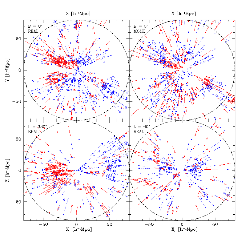
Figure 1: Radial peculiar velocities of “objects” in the Mark III catalog. The real data are shown in slices of $\pm 20^{\circ}$ about three planes: the Supergalactic plane ($B=0^{\circ}$) and two perpendicular planes, at $L=330^{\circ}$ and $60^{\circ}$. The coordinate $X_{\rm r}$ is either $X$, or $X$ rotated by $-30^{\circ}$ or $60^{\circ}$. Mock data are shown in comparison, but only about the Supergalactic plane (top-right panel). Distances and velocities are in $\,h^{-1}{\rm Mpc}$. The area of each symbol marking the object position is proportional to the object richness in galaxies. Solid and dashed lines distinguish outgoing and incoming radial velocities. The positions and velocities are corrected for Malmquist bias.

The main purpose of grouping in the Mark III catalog is to reduce the random error per object, and thus automatically reduce the resulting Malmquist bias (§ 7 below). The grouping procedure is described in detail in Willick et al. (1996). Galaxies were assigned to groups according to their proximity in angular position and in redshift. Proximity in inferred distance was used as a secondary criterion. The final grouped Mark III catalog consists of $\sim\!1200$ “objects” — single galaxies, groups and clusters.

Figure 1 illustrates the spatial distribution of objects in the Mark III catalog and their radial peculiar velocities in three orthogonal slices. One notices the poor coverage of the Galactic Zone of Avoidance (ZoA, about $Y=0$) and at large distances. The Supergalactic plane ($B=0^{\circ}$) and the plane $L=330^{\circ}$ both cut through the Great Attractor (GA, $X<0$) and Perseus Pisces (PP, $X>0$ and $Y<0$) regions where the streaming motions are large compared to the perpendicular plane, $L=60^{\circ}$.

Despite the careful effort made in the construction of the Mark III data, some galaxies are left that could be regarded as outliers, either because of observational errors or because they are indeed eccentric galaxies not obeying the TF relation. We make an additional effort to exclude such outliers using an iterative procedure based on the deviation of the inferred object peculiar velocity from the smoothed underlying velocity field at the location of that object. In each iteration, the data go through the smoothing procedure, and an object at $\kern-0.24994pt\hbox{$x$}\kern-5.71527pt\kern 0.50003pt\hbox{$x$}\kern-5.71527pt\kern-0.24994pt\raise 0.43304pt\hbox{$x$}_{i}$ is rejected if its peculiar velocity $u_{i}$ deviates from the smoothed velocity $u(\kern-0.24994pt\hbox{$x$}\kern-5.71527pt\kern 0.50003pt\hbox{$x$}\kern-5.71527pt\kern-0.24994pt\raise 0.43304pt\hbox{$x$}_{i})$ by more than $4(\Delta d+200\,{\rm km}\,{\rm s}^{-1})$, where the first term refers to the random distance error of the object and the second is an estimate of the dispersion velocity of field galaxies. In the end, only 3 galaxies are rejected from the Mark III data by applying this criterion.

In a recent analysis (Willick & Strauss 1998, VELMOD2, hereafter VM2), a revised calibration has been proposed for the TF zero points in the Mark III datasets that cover the Perseus-Pisces region, based on maximizing the agreement with the peculiar velocities predicted by the IRAS 1.2 Jy redshift survey. We test below the effects of this revised calibration on the reconstructed fields (§ 9.5).

3 MOCK CATALOGS

The POTENT method is tested using artificial catalogs based on an $N$-body simulation, which are described in detail in Kolatt et al. (1996). We present here only a brief summary.

A special effort has been made to generate a simulation that mimics the actual large-scale structure in the real universe about the Local Group, in order to take into account possible dependencies of the errors on the underlying signal. The present-day density field, smoothed with a Gaussian of radius $5\,h^{-1}{\rm Mpc}$ (G5), is taken to be the G5 density of IRAS 1.2 Jy galaxies as reconstructed by the method described in Sigad et al. (1998), assuming $\Omega=1$ and no biasing ($b_{\scriptscriptstyle\rm IRAS}=1$). The field is evolved back in time to remove non-linear effects by integrating the Zel’dovich-Bernoulli equation of Nusser & Dekel (1992). Remaining non-Gaussian features are removed by rank-preserving “Gaussianization” (Weinberg 1991), and artificial structure on scales smaller than the smoothing length is added using the method of constrained realizations (Hoffman & Ribak 1991), with the power spectrum of the IRAS 1.2 Jy survey (Fisher et al. 1993) as a prior model. The resulting density field is fed as initial conditions to a PM $N$-body code (Bertschinger & Gelb 1991), which then follows the forward non-linear evolution under gravity with $\Omega=1$. The present epoch is defined by an rms density fluctuation of $\sigma_{8}=0.7$ at a top-hat smoothing of radius $8\,h^{-1}{\rm Mpc}$, consistent with the value observed for IRAS galaxies and $b_{\scriptscriptstyle\rm IRAS}=1$ (Fisher et al. 1994). The periodic box of side $256\,h^{-1}{\rm Mpc}$ is simulated with a $128^{3}$ force grid and $128^{3}$ particles.

Figure 2 displays the particles in a slice of the simulation, of thickness $\pm 10\,h^{-1}{\rm Mpc}$ about the Supergalactic plane. It shows the familiar main features of the Great Attractor, Perseus-Pisce, and the extended low-density region in between. The fine sub-structure mimics the true rich clusters but it also contains a certain random element. The G12-smoothed density field is also marked, and is compared with the original, G12 fluctuation field of IRAS 1.2 Jy galaxies.

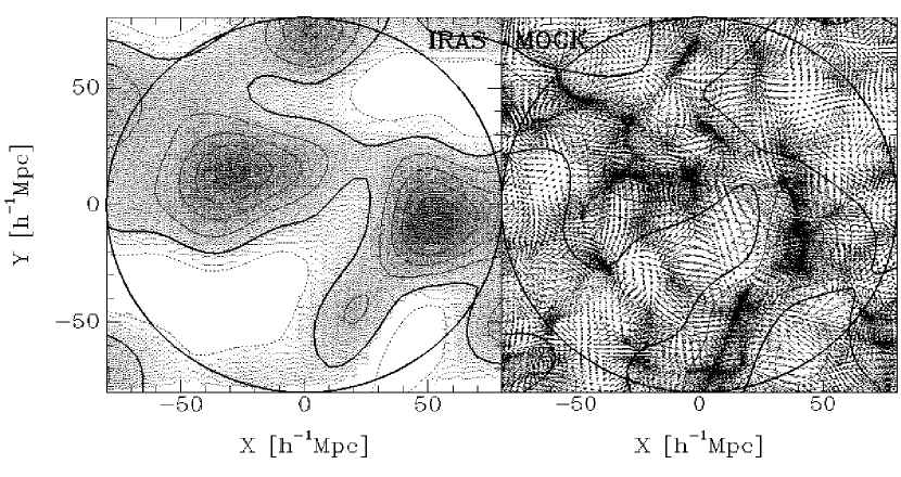
Figure 2: The simulation in the Supergalactic plane. The G12 density fluctuation field of IRAS 1.2 Jy galaxies (left) is compared to the corresponding density field in the simulation (right), which is overlaid on top of the particle distribution in a slice of thickness $\pm 10\,h^{-1}{\rm Mpc}$ about the plane. The contour spacing is $0.2$, with positive contours solid, negative contours dashed, and the zero contour heavy. Distances are in $\,h^{-1}{\rm Mpc}$. The LG is at the center. The GA is on the left and PP on the right.

In a second step that is repeated 10 times with different sets of random-numbers, “galaxies” are identified in the simulation, assigned their relevant physical properties, and then “observed” to make mock catalogs that include the same errors and selection effects as in the Mark III data. Each of the $N$-body particles is considered a galaxy candidate and is identified as an elliptical or a spiral depending on the local neighborhood density of particles (following Dressler 1980). Rich clusters are identified, mimicking the cluster samples in the real Mark III data, and the remaining particles are left as candidates for field galaxies. The galaxies are assigned internal velocities $\eta$ drawn at random  from the observed $\eta$ distribution function (corresponding to the observed “Schechter” galaxy luminosity function). A Tully-Fisher (or $D_{n}$-$\sigma$) relation is assumed, and absolute magnitudes $M$ are randomly  scattered about the TF value, $M_{\scriptscriptstyle\rm TF}(\eta)$, following a Gaussian distribution of width appropriate to the corresponding subset of the Mark III catalog. Field galaxies are selected in the angular regions corresponding to each of the sub-samples, with the appropriate magnitude limits and redshift cutoffs. This procedure amounts to a random selection of galaxies (as well as their physical properties) that mimics the statistical properties of the observed sample. The only feature of the observational procedure that is not simulated in this process is the error in the calibration of the TF relations, including the uncertainties in matching the zero points of the individual data samples in the unified Mark III catalog.

These data are used to infer TF distances to all the galaxies in each of the random mock realizations. The “observed” redshifts are taken to be the true velocities of the particles in the simulation. Finally, the galaxies selected are grouped using the same code used for the real data, and then corrected for Malmquist bias as in § 7 below, using the galaxy number density profile $n(r)$ as derived from randomly selected mock IRAS catalogs (from Sigad et al. 1998).

The top-right panel of Figure 1 shows the distribution of objects and their radial peculiar velocities in one random mock catalog, projected from a slice of $\pm 20^{\circ}$ about the Supergalactic plane into the plane. It resembles statistically the corresponding map of the real data.

4 STATISTICS FOR EVALUATING A RECONSTRUCTION

Before we embark on a detailed description of the POTENT algorithm, we first define the statistics needed for the testing procedure.

We use the $N$-body simulation and mock catalogs for evaluating the success of a reconstruction. The target for reconstruction is a true field $T(\kern-0.24994pt\hbox{$x$}\kern-5.71527pt\kern 0.50003pt\hbox{$x$}\kern-5.71527pt\kern-0.24994pt\raise 0.43304pt\hbox{$x$})$ (e.g., the density field, potential field, or any component of the velocity field), smoothed with a given window directly from the underlying particles of the simulation. The reconstruction from each mock catalog provides a corresponding POTENT field $P(\kern-0.24994pt\hbox{$x$}\kern-5.71527pt\kern 0.50003pt\hbox{$x$}\kern-5.71527pt\kern-0.24994pt\raise 0.43304pt\hbox{$x$})$. The quality of the reconstruction is evaluated by comparing these fields both locally and globally inside a given reference volume.

In the current paper, the comparison is first performed visually via maps in the Supergalactic plane out to $80\,h^{-1}{\rm Mpc}$, and then quantitatively at points of a uniform grid within a smaller reference volume. We focus here on the reconstruction of the mass-density field, smoothed with a Gaussian window of radius $10$-$12\,h^{-1}{\rm Mpc}$, within a reference volume of an effective radius $30$-$50\,h^{-1}{\rm Mpc}$ about the Local Group (see § 8.1 for a more specific definition of the reference volume).

For testing cases with noisy input, POTENT is applied to each of $M$ ($\sim 10$) random mock catalogs to yield a series of $M$ noisy POTENT fields $\{P_{m}(\kern-0.24994pt\hbox{$x$}\kern-5.71527pt\kern 0.50003pt\hbox{$x$}\kern-5.71527pt\kern-0.24994pt\raise 0.43304pt\hbox{$x$})\}_{m=1}^{M}$. The rms scatter of these fields about the true field $T(\kern-0.24994pt\hbox{$x$}\kern-5.71527pt\kern 0.50003pt\hbox{$x$}\kern-5.71527pt\kern-0.24994pt\raise 0.43304pt\hbox{$x$})$ provides the error field $\sigma_{\rm tot}(\kern-0.24994pt\hbox{$x$}\kern-5.71527pt\kern 0.50003pt\hbox{$x$}\kern-5.71527pt\kern-0.24994pt\raise 0.43304pt\hbox{$x$})$. This error contains both systematic and random components. The systematic error field is given by $\bar{P}(\kern-0.24994pt\hbox{$x$}\kern-5.71527pt\kern 0.50003pt\hbox{$x$}\kern-5.71527pt\kern-0.24994pt\raise 0.43304pt\hbox{$x$})-T(\kern-0.24994pt\hbox{$x$}\kern-5.71527pt\kern 0.50003pt\hbox{$x$}\kern-5.71527pt\kern-0.24994pt\raise 0.43304pt\hbox{$x$})$, where $\bar{P}(\kern-0.24994pt\hbox{$x$}\kern-5.71527pt\kern 0.50003pt\hbox{$x$}\kern-5.71527pt\kern-0.24994pt\raise 0.43304pt\hbox{$x$})$ is the average over the noisy fields $\{P_{m}(\kern-0.24994pt\hbox{$x$}\kern-5.71527pt\kern 0.50003pt\hbox{$x$}\kern-5.71527pt\kern-0.24994pt\raise 0.43304pt\hbox{$x$})\}$ (we hereafter denote averaging over the noisy realizations by an over-line). In test cases with no random selection of objects and no random errors, there is no need to average over realizations and the bias field is simply $P(\kern-0.24994pt\hbox{$x$}\kern-5.71527pt\kern 0.50003pt\hbox{$x$}\kern-5.71527pt\kern-0.24994pt\raise 0.43304pt\hbox{$x$})-T(\kern-0.24994pt\hbox{$x$}\kern-5.71527pt\kern 0.50003pt\hbox{$x$}\kern-5.71527pt\kern-0.24994pt\raise 0.43304pt\hbox{$x$})$.

The interpretation of the various statistics that are defined in this section will become clearer when associated with one of the scatter diagrams of $P$ (or $\bar{P}$) versus $T$ in the following sections.

The typical systematic error within the reference volume is estimated by the rms of the residuals over the volume (i.e., over uniform grid points):

$$\sigma_{\rm sys}^{2}\equiv\langle[\bar{P}(\kern-0.24994pt\hbox{$x$}\kern-5.71527pt\kern 0.50003pt\hbox{$x$}\kern-5.71527pt\kern-0.24994pt\raise 0.43304pt\hbox{$x$})-T(\kern-0.24994pt\hbox{$x$}\kern-5.71527pt\kern 0.50003pt\hbox{$x$}\kern-5.71527pt\kern-0.24994pt\raise 0.43304pt\hbox{$x$})]^{2}\rangle\ .$$ (5)

(We hereafter denote spatial averaging by angular parentheses.) A meaningful measure that allows a comparative evaluation of reconstructions with different smoothings is $\epsilon_{\rm sys}\equiv\sigma_{\rm sys}/\sigma_{\scriptscriptstyle\rm T}$, where $\sigma_{\scriptscriptstyle\rm T}$ is the standard deviation of the true field.

The systematic error can be decomposed into global and local components by performing a linear regression of $\bar{P}$ on $T$:

$$\bar{P}=sT+c\ .$$ (6)

The constant $c$ is typically small. (If the volume is big enough such that cosmic scatter is negligible, one can assume $\langle T\rangle=0$ and set $c$ to zero by enforcing $\langle\bar{P}\rangle=0$.) The slope of the regression line, $s=\langle(\bar{P}-\langle\bar{P}\rangle)(T-\langle T\rangle)\rangle/\sigma_{\scriptscriptstyle\rm T}^{2}$, characterizes the global  bias; a deviation of $s$ from unity can be interpreted as an error in the effective smoothing of the reconstruction. Note that such a global systematic error could be harmful when the POTENT output is used for measuring cosmological parameters or is compared to other data, and it should therefore be kept small. One can crudely correct for such a bias in retrospect, provided it is sufficiently small (e.g., Dekel et al. 1993).

The scatter about the best-fit line characterizes the local  bias:

$$\sigma_{\rm loc}^{2}\equiv\langle[\bar{P}(\kern-0.24994pt\hbox{$x$}\kern-5.71527pt\kern 0.50003pt\hbox{$x$}\kern-5.71527pt\kern-0.24994pt\raise 0.43304pt\hbox{$x$})-sT(\kern-0.24994pt\hbox{$x$}\kern-5.71527pt\kern 0.50003pt\hbox{$x$}\kern-5.71527pt\kern-0.24994pt\raise 0.43304pt\hbox{$x$})-c]^{2}\rangle\ .$$ (7)

It is a bias  because the random noise has been removed from $\bar{P}$ by the averaging over the many mock catalogs. Again, this quantity becomes of more general interest when scaled into $\epsilon_{\rm loc}\equiv{\sigma_{\rm loc}/(s\sigma_{\scriptscriptstyle\rm T})}$. Equivalently, the same local bias can be characterized by the linear correlation coefficient, $r\equiv\langle(\bar{P}-\langle\bar{P}\rangle)(T-\langle T\rangle)\rangle/(\sigma_{\scriptscriptstyle\rm T}\sigma_{\scriptscriptstyle\rm\bar{P}})$, where $\sigma_{\scriptscriptstyle\rm\bar{P}}$ is the standard deviation of the average POTENT field. The simple relation between these two equivalent measures of local bias is

$$\epsilon_{\rm loc}^{2}=r^{-2}-1\ .$$ (8)

The whole systematic error is then characterized by the sum in quadrature of the local and global components:

$$\epsilon_{\rm sys}^{2}=s^{2}(r^{-2}-1)+(s-1)^{2}+{c^{2}\over\sigma_{\scriptscriptstyle\rm T}^{2}}$$ (9)

(assuming $\langle T\rangle=0$).

In each case, we list the parameters $s$, $r$ and $c$, plus the corresponding $\sigma_{\scriptscriptstyle\rm T}$, as measures of systematic errors inside a reference volume. The other parameters can be derived from these using the above relations. A perfect reconstruction is characterized by $s=r=1$ and $c=0$, while a failure is diagnosed by a large deviations from these values.

The field of random  errors, when relevant, is derived from the series of noisy POTENT fields $\{P_{m}(\kern-0.24994pt\hbox{$x$}\kern-5.71527pt\kern 0.50003pt\hbox{$x$}\kern-5.71527pt\kern-0.24994pt\raise 0.43304pt\hbox{$x$})\}$ by the rms residual relative to the average field:

$$\sigma_{\rm ran}^{2}(\kern-0.24994pt\hbox{$x$}\kern-5.71527pt\kern 0.50003pt\hbox{$x$}\kern-5.71527pt\kern-0.24994pt\raise 0.43304pt\hbox{$x$})\equiv\overline{[P_{m}(\kern-0.24994pt\hbox{$x$}\kern-5.71527pt\kern 0.50003pt\hbox{$x$}\kern-5.71527pt\kern-0.24994pt\raise 0.43304pt\hbox{$x$})-\bar{P}(\kern-0.24994pt\hbox{$x$}\kern-5.71527pt\kern 0.50003pt\hbox{$x$}\kern-5.71527pt\kern-0.24994pt\raise 0.43304pt\hbox{$x$})]^{2}}\ .$$ (10)

The corresponding field of total error is defined by the rms residual relative to the true  field:

$$\sigma_{\rm tot}^{2}(\kern-0.24994pt\hbox{$x$}\kern-5.71527pt\kern 0.50003pt\hbox{$x$}\kern-5.71527pt\kern-0.24994pt\raise 0.43304pt\hbox{$x$})\equiv\overline{[P_{m}(\kern-0.24994pt\hbox{$x$}\kern-5.71527pt\kern 0.50003pt\hbox{$x$}\kern-5.71527pt\kern-0.24994pt\raise 0.43304pt\hbox{$x$})-T(\kern-0.24994pt\hbox{$x$}\kern-5.71527pt\kern 0.50003pt\hbox{$x$}\kern-5.71527pt\kern-0.24994pt\raise 0.43304pt\hbox{$x$})]^{2}}\ .$$ (11)

Either $\sigma_{\rm ran}(\kern-0.24994pt\hbox{$x$}\kern-5.71527pt\kern 0.50003pt\hbox{$x$}\kern-5.71527pt\kern-0.24994pt\raise 0.43304pt\hbox{$x$})$ or $\sigma_{\rm tot}(\kern-0.24994pt\hbox{$x$}\kern-5.71527pt\kern 0.50003pt\hbox{$x$}\kern-5.71527pt\kern-0.24994pt\raise 0.43304pt\hbox{$x$})$ can be used in further analysis using POTENT output. The typical values of these errors within a reference volume are estimated by spatial averaging:

$$\sigma_{\rm ran}^{2}\equiv\langle\sigma_{\rm ran}^{2}(\kern-0.24994pt\hbox{$x$}\kern-5.71527pt\kern 0.50003pt\hbox{$x$}\kern-5.71527pt\kern-0.24994pt\raise 0.43304pt\hbox{$x$})\rangle\ ,$$ (12)

$$\sigma_{\rm tot}^{2}\equiv\langle\sigma_{\rm tot}^{2}(\kern-0.24994pt\hbox{$x$}\kern-5.71527pt\kern 0.50003pt\hbox{$x$}\kern-5.71527pt\kern-0.24994pt\raise 0.43304pt\hbox{$x$})\rangle=\sigma_{\rm sys}^{2}+\sigma_{\rm ran}^{2}\ .$$ (13)

The parameters for evaluating the random and total errors are finally quoted as $\epsilon_{\rm ran}\equiv\sigma_{\rm ran}/\sigma_{\scriptscriptstyle\rm T}$ and $\epsilon_{\rm tot}\equiv\sigma_{\rm tot}/\sigma_{\scriptscriptstyle\rm T}$.

In the above statistics, the volume averages are all unweighted; the grid points within the reference volume are treated as equals. However, further analysis using POTENT output may prefer to give more weight to points in which the reconstruction is of higher quality. For example, in the POTIRAS comparison (Sigad et al. 1998), the POTENT densities were weighted by $\sigma_{\rm tot}^{-2}$, including the random and the systematic errors. In the tests presented here, however, we prefer to use $\sigma_{\rm ran}^{-2}$ as weights and as flags of quality reconstruction. This is because $\sigma_{\rm ran}$ does not explicitly depend on the true field, and because the weighting by $\sigma_{\rm tot}^{-2}$ would artificially reduce the signal of systematic errors which we wish to identify. We thus define weighted statistics, $s_{\rm w}$, $r_{\rm w}$, etc., in a way analogous to the above statistics $s$, $r$, etc., except that the volume averaging is replaced by weighted  volume averaging, with weights $\sigma_{\rm ran}^{-2}$. This weighting, like all the above statistics, is specific to the given dataset, which is currently the Mark III catalog.

5 POTENTIAL ANALYSIS AND DENSITY RECONSTRUCTION

The most straightforward stage of POTENT is the potential analysis starting from a smoothed radial peculiar velocity field, $u(\kern-0.24994pt\hbox{$x$}\kern-5.71527pt\kern 0.50003pt\hbox{$x$}\kern-5.71527pt\kern-0.24994pt\raise 0.43304pt\hbox{$x$})$. This stage consists of applying the ansatz of potential flow, equation (1), to recover the velocity potential and the three-dimensional velocity field, $\kern-0.24994pt\hbox{$v$}\kern-5.20601pt\kern 0.50003pt\hbox{$v$}\kern-5.20601pt\kern-0.24994pt\raise 0.43304pt\hbox{$v$}(\kern-0.24994pt\hbox{$x$}\kern-5.71527pt\kern 0.50003pt\hbox{$x$}\kern-5.71527pt\kern-0.24994pt\raise 0.43304pt\hbox{$x$})$, and then deriving the underlying density fluctuation field $\delta(\kern-0.24994pt\hbox{$x$}\kern-5.71527pt\kern 0.50003pt\hbox{$x$}\kern-5.71527pt\kern-0.24994pt\raise 0.43304pt\hbox{$x$})$ by an adequate approximation to GI in the mildly non-linear regime. We test this part of the method assuming the true smoothed velocity field as input.

5.1 Potential Analysis

In practice, the smoothed radial velocity field is computed (§ 6 below) at the points of a spherical grid of 24 equal radial bins out to $R_{\rm max}=80\,h^{-1}{\rm Mpc}$, 48 equal latitude ($B$) bins in the range $\pm\pi/2$, and $96\times\cos B$ roughly-equal longitude bins between 0 and $2\pi$. The potential at the origin is arbitrarily fixed to zero, and the potential at every other grid point is computed by cubic spline integration of $u(\kern-0.24994pt\hbox{$x$}\kern-5.71527pt\kern 0.50003pt\hbox{$x$}\kern-5.71527pt\kern-0.24994pt\raise 0.43304pt\hbox{$x$})$ along the radial rays of the spherical grid, equation (1).

The potential is then interpolated by linear cloud-in-cell (CIC) onto the points of a cubic grid of $2.5\,h^{-1}{\rm Mpc}$ spacing (positioned such that there is a grid point at the origin). The partial derivatives are computed by finite differencing to yield the three-dimensional velocity components via $\kern-0.24994pt\hbox{$v$}\kern-5.20601pt\kern 0.50003pt\hbox{$v$}\kern-5.20601pt\kern-0.24994pt\raise 0.43304pt\hbox{$v$}\!=\!-\kern-0.24994pt\hbox{$\nabla$}\kern-8.33336pt\kern 0.50003pt\hbox{$\nabla$}\kern-8.33336pt\kern-0.24994pt\raise 0.43304pt\hbox{$\nabla$}\Phi$. The second partial derivatives of the potential are computed in a similar way for the purpose of approximating the density fluctuation field.

5.2 From Velocity to Density

In the linear approximation to GI, the underlying mass-density fluctuation field is derived from the velocity field via one more differentiation, $\delta_{0}=-f(\Omega)^{-1}\kern-0.24994pt\hbox{$\nabla$}\kern-8.33336pt\kern 0.50003pt\hbox{$\nabla$}\kern-8.33336pt\kern-0.24994pt\raise 0.43304pt\hbox{$\nabla$}\cdot\kern-0.24994pt\hbox{$v$}\kern-5.20601pt\kern 0.50003pt\hbox{$v$}\kern-5.20601pt\kern-0.24994pt\raise 0.43304pt\hbox{$v$}$, where $f(\Omega)\simeq\Omega^{0.6}$ (e.g., Peebles 1980). However, the linear approximation is limited to the small dynamic range between a few tens of megaparsecs and the $\sim\!100\,h^{-1}{\rm Mpc}$ extent of the current samples. The current sampling of galaxies enables reliable dynamical analysis with a smoothing radius as small as $\sim\!10\,h^{-1}{\rm Mpc}$ (or even smaller in more limited regions), where $|\kern-0.24994pt\hbox{$\nabla$}\kern-8.33336pt\kern 0.50003pt\hbox{$\nabla$}\kern-8.33336pt\kern-0.24994pt\raise 0.43304pt\hbox{$\nabla$}\cdot\kern-0.24994pt\hbox{$v$}\kern-5.20601pt\kern 0.50003pt\hbox{$v$}\kern-5.20601pt\kern-0.24994pt\raise 0.43304pt\hbox{$v$}|$ reaches values larger than unity such that non-linear effects play a role. Therefore, the derivation of the density field requires an approximate solution to the equations of GI in the mildly non-linear regime.

We appeal to the Zel’dovich (1970) approximation, which is known to be a successful tool in the mildly non-linear regime. Substituting an Eulerian version of the Zel’dovich approximation in the continuity equation yields (Nusser et al. 1991)

$$\delta_{c}(\kern-0.24994pt\hbox{$x$}\kern-5.71527pt\kern 0.50003pt\hbox{$x$}\kern-5.71527pt\kern-0.24994pt\raise 0.43304pt\hbox{$x$})=\|\kern-0.24994pt\hbox{I}\kern-3.61111pt\kern 0.50003pt\hbox{I}\kern-3.61111pt\kern-0.24994pt\raise 0.43304pt\hbox{I}-f^{-1}{\partial\kern-0.24994pt\hbox{$v$}\kern-5.20601pt\kern 0.50003pt\hbox{$v$}\kern-5.20601pt\kern-0.24994pt\raise 0.43304pt\hbox{$v$}/\partial\kern-0.24994pt\hbox{$x$}\kern-5.71527pt\kern 0.50003pt\hbox{$x$}\kern-5.71527pt\kern-0.24994pt\raise 0.43304pt\hbox{$x$}}\|-1\ ,$$ (14)

where the bars denote the Jacobian determinant and III is the unit matrix.

Figure 3 (middle panel), based on $N$-body simulations (Ganon et al. 1998), demonstrates the performance of this approximation in comparison with the linear approximation (left panel). The densities derived from the G12-smoothed peculiar velocity field are compared at the points of a uniform grid to the true G12 density field in the simulation. Note that the residuals are $\sim 0.05$ or less. The error $\epsilon_{\rm sys}$ improves from 0.099 to 0.071. The approximation does a good job for $\delta\geq 0$, but it tends to be a slight overestimate in the negative tail of $\delta<0$, and it becomes worse as one approaches $\delta\sim-1$ (see also Mancinelli et al. 1994; Mancinelli & Yahil 1995).

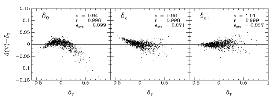
Figure 3: Approximations to GI in the mildly non-linear regime. The density fluctuation fields as derived from the partial derivatives of the peculiar velocity field are compared point by point to the true density field in the simulation ($\delta_{\scriptscriptstyle\rm T}$). The smoothing is G12. The mean spacing between the sampled points is $24\,h^{-1}{\rm Mpc}$. The vertical scale is enlarged by a factor of $\sim 6$ compared to the horizontal scale. Error statistics are quoted (defined in § 4). Left: the linear approximation $\delta_{0}$. Middle: the Zel’dovich-continuity approximation $\delta_{c}$. Right: the improved approximation $\delta_{c+}$.

This approximation can be improved as follows. The Zel’dovich displacement is first order in $f^{-1}$ and $v$$v$$v$, and therefore the determinant in $\delta_{c}$ includes second- and third-order terms as well, involving sums of double and triple products of partial derivatives:

$$\delta_{c}=-f^{-1}\kern-0.24994pt\hbox{$\nabla$}\kern-8.33336pt\kern 0.50003pt\hbox{$\nabla$}\kern-8.33336pt\kern-0.24994pt\raise 0.43304pt\hbox{$\nabla$}\cdot\kern-0.24994pt\hbox{$v$}\kern-5.20601pt\kern 0.50003pt\hbox{$v$}\kern-5.20601pt\kern-0.24994pt\raise 0.43304pt\hbox{$v$}+f^{-2}\Delta_{2}+f^{-3}\Delta_{3}\ ,$$ (15)

where

$$\Delta_{2}(\kern-0.24994pt\hbox{$x$}\kern-5.71527pt\kern 0.50003pt\hbox{$x$}\kern-5.71527pt\kern-0.24994pt\raise 0.43304pt\hbox{$x$})=\sum_{i<j}\left[\left({\partial v_{i}\over\partial x_{j}}\right)^{2}-{\partial v_{i}\over\partial x_{i}}{\partial v_{j}\over\partial x_{j}}\right]\ ,$$ (16)

and

$$\Delta_{3}(\kern-0.24994pt\hbox{$x$}\kern-5.71527pt\kern 0.50003pt\hbox{$x$}\kern-5.71527pt\kern-0.24994pt\raise 0.43304pt\hbox{$x$})=\sum_{i,j,k}\left[{\partial v_{i}\over\partial x_{i}}{\partial v_{j}\over\partial x_{k}}{\partial v_{k}\over\partial x_{j}}-{\partial v_{1}\over\partial x_{i}}{\partial v_{2}\over\partial x_{j}}{\partial v_{3}\over\partial x_{k}}\right]\ ,$$ (17)

in which $i,j,k$ run over the three cyclic permutations of $1,2,3$. The $\delta_{c}$ approximation can be improved by slight adjustments to the coefficients of the three terms in equation (15),

$$\delta_{c+}=-(1+\epsilon_{1})f^{-1}\kern-0.24994pt\hbox{$\nabla$}\kern-8.33336pt\kern 0.50003pt\hbox{$\nabla$}\kern-8.33336pt\kern-0.24994pt\raise 0.43304pt\hbox{$\nabla$}\cdot\kern-0.24994pt\hbox{$v$}\kern-5.20601pt\kern 0.50003pt\hbox{$v$}\kern-5.20601pt\kern-0.24994pt\raise 0.43304pt\hbox{$v$}+(1+\epsilon_{2})f^{-2}\Delta_{2}+(1+\epsilon_{3})f^{-3}\Delta_{3}\ .$$ (18)

These coefficients were empirically tuned to provide best fits for a family of CDM simulations of G12 smoothing over the whole range of $\delta$ values, with $\epsilon_{1}=0.06$, $\epsilon_{2}=-0.13$ and $\epsilon_{3}=-0.3$. Figure 3 (right panel) demonstrates the improvement in $\delta_{c+}$ over $\delta_{c}$ for G12 smoothing. The global systematic errors in the tails, that were apparent for $\delta_{0}$ and $\delta_{c}$, are now practically gone; $s=1.01$ and $r=0.99$. The typical local error is down to $\epsilon_{\rm sys}=0.057$.

The $\delta_{c+}$ approximation is found to be robust to quantities that are unknown a priori such as (a) the value of $\Omega$ in the range $0.3-1.0$, (b) the shape of the power spectrum within the general CDM family, allowing for a nonzero cosmological constant as well as a slight tilt in the power spectrum on large scales (tested for the power index $n$ in the range $0.6-1.0$), and (c) the degree of non-linearity as determined by the fluctuation amplitude and the smoothing scale (Ganon et al. 1998). We adopt $\delta_{c+}$ as our standard approximation in POTENT.

5.3 Testing POTENT with Ideal Data

We first use the simulation to evaluate the POTENT reconstruction from ideal data with dense and uniform sampling and no distance errors.

The true, G-smoothed radial velocity field of the simulation, which serves as input for this test, is computed as follows. The three-dimensional field is first computed at the points of a fine cubic grid of $2\,h^{-1}{\rm Mpc}$ spacing by applying to the particle velocities a Gaussian smoothing of equally small radius, $r_{s}=2\,h^{-1}{\rm Mpc}$. The velocity field smoothed with a Gaussian of much larger radius $R_{\rm s}$, say, G12, is then computed by FFT. This G-smoothed velocity field is finally interpolated by CIC onto the desired spherical grid of the potential integration, and the radial components serve as input for POTENT in the current test.

Figure 4 compares the density fluctuation field recovered by POTENT in this ideal case, $\delta_{\scriptscriptstyle\rm P}$, with the target true field of the simulation, $\delta_{\scriptscriptstyle\rm T}$, for both G10 and G12 smoothings. The comparison is done both via maps in the Supergalactic plane and point by point on a cubic grid of spacing $5\,h^{-1}{\rm Mpc}$ inside a comparison sphere of radius $40\,h^{-1}{\rm Mpc}$. In order to make this scatter plot less crowded (and similar plots below), only a random subsample containing 20% of the grid points is shown, with a mean separation of $8.5\,h^{-1}{\rm Mpc}$.

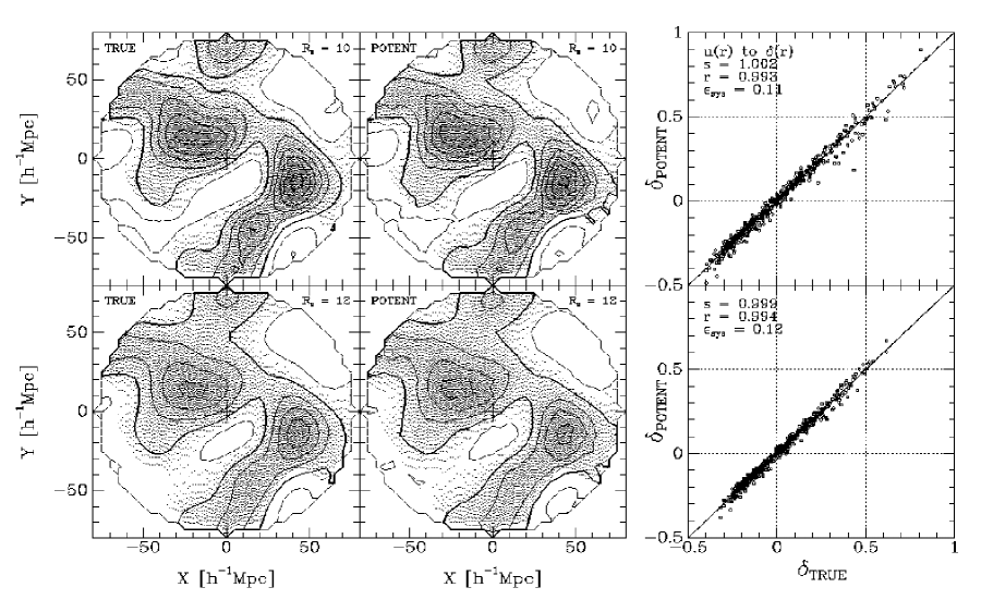
Figure 4: Reconstruction from ideal mock data. The mass density fluctuation field as reconstructed by POTENT from the exact radial velocity field of the simulation, compared to the true density field. Smoothing is G10 (top) or G12 (bottom). Contours are as in Figure 2. A comparison to the true field is shown (right) inside a sphere of radius $40\,h^{-1}{\rm Mpc}$, at points sampled with a mean separation of $8.5\,h^{-1}{\rm Mpc}$. Statistics measuring the typical systematic errors are quoted.

As explained in § 4, the residuals in this scatter plot of $\delta_{\scriptscriptstyle\rm P}$ versus $\delta_{\scriptscriptstyle\rm T}$ are purely systematic errors (as the input is free of random noise in this case). Their global and local components as measured by $s$ and $r$ are shown in the figure and in Table 2.

The success of the reconstruction in this case of no noise is excellent. With $s$ deviating from unity by only a small fraction of a percent, essentially no global bias is introduced by the potential analysis. The small scatter of only $11-12\%$ of $\sigma_{\scriptscriptstyle\rm T}$, which is reflected in the $<1\%$ deviation of $r$ from unity, is a result of the accumulating effects of (a) numerical errors due to the finite grids used, (b) scatter about the non-linear approximation $\delta_{c+}$, and (c) small deviations from potential flow at these smoothing scales. The latter can be estimated by the rms of $\kern-0.24994pt\hbox{$\nabla$}\kern-8.33336pt\kern 0.50003pt\hbox{$\nabla$}\kern-8.33336pt\kern-0.24994pt\raise 0.43304pt\hbox{$\nabla$}\!\times\!\kern-0.24994pt\hbox{$v$}\kern-5.20601pt\kern 0.50003pt\hbox{$v$}\kern-5.20601pt\kern-0.24994pt\raise 0.43304pt\hbox{$v$}$ in the box, which is 4.4% of the density $\sigma_{\scriptscriptstyle\rm T}$ for G12, and 5.4% for G10. All these errors are negligible compared to those associated with computing the smoothed radial field $u(\kern-0.24994pt\hbox{$x$}\kern-5.71527pt\kern 0.50003pt\hbox{$x$}\kern-5.71527pt\kern-0.24994pt\raise 0.43304pt\hbox{$x$})$ from the sparse, non-uniform and noisy data. These are discussed next.

6 THE SMOOTHING PROCEDURE

The most difficult step in the POTENT procedure is the interpolation and smoothing of the observed radial peculiar velocities $u_{i}$ at the inferred object positions $\kern-0.24994pt\hbox{$x$}\kern-5.71527pt\kern 0.50003pt\hbox{$x$}\kern-5.71527pt\kern-0.24994pt\raise 0.43304pt\hbox{$x$}_{i}$, with errors $\sigma_{i}$, onto a radial velocity field at grid points, $u(\kern-0.24994pt\hbox{$x$}\kern-5.71527pt\kern 0.50003pt\hbox{$x$}\kern-5.71527pt\kern-0.24994pt\raise 0.43304pt\hbox{$x$})$, which serves as input for the potential analysis described above. The aim of this procedure is to mimic volume-weighted smoothing of the three-dimensional velocity field $\kern-0.24994pt\hbox{$v$}\kern-5.20601pt\kern 0.50003pt\hbox{$v$}\kern-5.20601pt\kern-0.24994pt\raise 0.43304pt\hbox{$v$}(\kern-0.24994pt\hbox{$x$}\kern-5.71527pt\kern 0.50003pt\hbox{$x$}\kern-5.71527pt\kern-0.24994pt\raise 0.43304pt\hbox{$x$})$ with a spherical Gaussian window of radius $R_{\rm s}$. In the unrealistic case of dense and uniform sampling of the three components of $\kern-0.24994pt\hbox{$v$}\kern-5.20601pt\kern 0.50003pt\hbox{$v$}\kern-5.20601pt\kern-0.24994pt\raise 0.43304pt\hbox{$v$}(\kern-0.24994pt\hbox{$x$}\kern-5.71527pt\kern 0.50003pt\hbox{$x$}\kern-5.71527pt\kern-0.24994pt\raise 0.43304pt\hbox{$x$})$ with random noise only, the desired smoothed velocity would have simply been the best-fit bulk velocity of the data weighted by a spherical Gaussian about the window center. However, the limitations of the actual data introduce biases that present non-trivial complications.

The general idea of our smoothing procedure of the actual data about a grid point $\kern-0.24994pt\hbox{$x$}\kern-5.71527pt\kern 0.50003pt\hbox{$x$}\kern-5.71527pt\kern-0.24994pt\raise 0.43304pt\hbox{$x$}_{c}$ is that the smoothed radial velocity $u(\kern-0.24994pt\hbox{$x$}\kern-5.71527pt\kern 0.50003pt\hbox{$x$}\kern-5.71527pt\kern-0.24994pt\raise 0.43304pt\hbox{$x$}_{c})$ is taken to be the value at $\kern-0.24994pt\hbox{$x$}\kern-5.71527pt\kern 0.50003pt\hbox{$x$}\kern-5.71527pt\kern-0.24994pt\raise 0.43304pt\hbox{$x$}\!=\!\kern-0.24994pt\hbox{$x$}\kern-5.71527pt\kern 0.50003pt\hbox{$x$}\kern-5.71527pt\kern-0.24994pt\raise 0.43304pt\hbox{$x$}_{c}$ of the radial component of an appropriate local  velocity model $\kern-0.24994pt\hbox{$v$}\kern-5.20601pt\kern 0.50003pt\hbox{$v$}\kern-5.20601pt\kern-0.24994pt\raise 0.43304pt\hbox{$v$}(\alpha_{k};\kern-0.24994pt\hbox{$x$}\kern-5.71527pt\kern 0.50003pt\hbox{$x$}\kern-5.71527pt\kern-0.24994pt\raise 0.43304pt\hbox{$x$}\!-\!\kern-0.24994pt\hbox{$x$}\kern-5.71527pt\kern 0.50003pt\hbox{$x$}\kern-5.71527pt\kern-0.24994pt\raise 0.43304pt\hbox{$x$}_{c})$ with free parameters $\{\alpha_{k}\}$. These parameters are obtained by minimizing the weighted sum of residuals

$$-2\ln{\cal L}\propto\sum_{i}W_{i}\,[u_{i}-\hat{\kern-0.24994pt\hbox{$x$}\kern-5.71527pt\kern 0.50003pt\hbox{$x$}\kern-5.71527pt\kern-0.24994pt\raise 0.43304pt\hbox{$x$}}_{i}\cdot\kern-0.24994pt\hbox{$v$}\kern-5.20601pt\kern 0.50003pt\hbox{$v$}\kern-5.20601pt\kern-0.24994pt\raise 0.43304pt\hbox{$v$}(\alpha_{k};\kern-0.24994pt\hbox{$x$}\kern-5.71527pt\kern 0.50003pt\hbox{$x$}\kern-5.71527pt\kern-0.24994pt\raise 0.43304pt\hbox{$x$}_{i})]^{2}$$ (19)

within an appropriate local window function $W_{i}\!=\!W(\kern-0.24994pt\hbox{$x$}\kern-5.71527pt\kern 0.50003pt\hbox{$x$}\kern-5.71527pt\kern-0.24994pt\raise 0.43304pt\hbox{$x$}_{i},\kern-0.24994pt\hbox{$x$}\kern-5.71527pt\kern 0.50003pt\hbox{$x$}\kern-5.71527pt\kern-0.24994pt\raise 0.43304pt\hbox{$x$}_{c})$. The basic component of the window function is a spherical Gaussian of radius $R_{\rm s}$, $W_{i}\propto\exp[-(\kern-0.24994pt\hbox{$x$}\kern-5.71527pt\kern 0.50003pt\hbox{$x$}\kern-5.71527pt\kern-0.24994pt\raise 0.43304pt\hbox{$x$}_{i}-\kern-0.24994pt\hbox{$x$}\kern-5.71527pt\kern 0.50003pt\hbox{$x$}\kern-5.71527pt\kern-0.24994pt\raise 0.43304pt\hbox{$x$}_{c})^{2}/2R_{\rm s}^{2}]$. It is modified, together with the local velocity model, in an effort to minimize the biases described below. Note that if the errors were Gaussian and $W_{i}\!\propto\!\sigma_{i}^{-2}$, then ${\cal L}$ would have been the formal likelihood; it remains only an approximation to the likelihood in our case where the errors are closer to a log-normal distribution, and it may be carried further away from the likelihood by the additional weighting.

6.1 Tensor Window Bias

In general, the radial directions from the origin (the Local Group) to the objects ($\hat{\kern-0.24994pt\hbox{$x$}\kern-5.71527pt\kern 0.50003pt\hbox{$x$}\kern-5.71527pt\kern-0.24994pt\raise 0.43304pt\hbox{$x$}}_{i}$) do not coincide with the radial direction to the window center ($\hat{\kern-0.24994pt\hbox{$x$}\kern-5.71527pt\kern 0.50003pt\hbox{$x$}\kern-5.71527pt\kern-0.24994pt\raise 0.43304pt\hbox{$x$}}_{c}$) at which we try to obtain the smoothed radial velocity. Therefore, unless the window radius is negligible compared to its distance from the origin ($R_{\rm s}\ll r_{c}$), the radial velocities cannot be averaged as scalars, and one has to appeal to a fit of a local 3D velocity model, as described above. The original POTENT procedure of DBF used the simplest model within each window, i.e., a local bulk velocity with three parameters, $\kern-0.24994pt\hbox{$v$}\kern-5.20601pt\kern 0.50003pt\hbox{$v$}\kern-5.20601pt\kern-0.24994pt\raise 0.43304pt\hbox{$v$}(\kern-0.24994pt\hbox{$x$}\kern-5.71527pt\kern 0.50003pt\hbox{$x$}\kern-5.71527pt\kern-0.24994pt\raise 0.43304pt\hbox{$x$})\!=\!\kern-0.24994pt\hbox{$B$}\kern-8.0868pt\kern 0.50003pt\hbox{$B$}\kern-8.0868pt\kern-0.24994pt\raise 0.43304pt\hbox{$B$}$. For such a model the solution can be expressed explicitly in terms of a tensor window function, and the minimization procedure can be replaced by a simple matrix inversion (BD; DBF; BFDFB).

Unfortunately, an attempt to use a model that does not have enough degrees of freedom for a proper fit of the variations of the velocity field within a window is likely to lead to a biased result. As an example, consider an infall towards a point attractor at the center of the smoothing window, and in particular the converging velocity component in the plane transverse to the line of sight to the window center. For all tracers in that plane (except the window center), the radial (line-of-sight) components observed are all negative, leading to a best-fit bulk velocity within the window that would be erroneously interpreted as a radial velocity towards the origin (LG). Similarly, a transverse outflow pattern would be interpreted as a radial outflow away from the origin. Another bias arises from the fact that the tensorial correction to the spherical window has a conical symmetry, weighting more heavily objects that lie along radial rays that are closer to the radial ray through the window center, and thus distorting the effective window shape. We term these systematic effects “window bias” (WB).

Figure 5 (panel a) shows the WB in $u(\kern-0.24994pt\hbox{$x$}\kern-5.71527pt\kern 0.50003pt\hbox{$x$}\kern-5.71527pt\kern-0.24994pt\raise 0.43304pt\hbox{$x$})$ in the Supergalactic plane, resulting from G12 bulk-velocity (3-parameter) smoothing of unperturbed and uniformly-sampled radial velocities from the simulation. In the converging GA region (upper-left quadrant), the WB is as high as $-350\,{\rm km}\,{\rm s}^{-1}$. In the outflowing void in the foreground of PP (bottom right quadrant), it is about $+200\,{\rm km}\,{\rm s}^{-1}$.

Figure 5: Window bias in the velocity field in the Supergalactic Plane as a function of the local velocity model and the smoothing scale. The input data are the true high-resolution radial velocities of the simulation, sampled uniformly at grid points of spacing $6\,h^{-1}{\rm Mpc}$. Distances and velocities are in $\,h^{-1}{\rm Mpc}=100\,{\rm km}\,{\rm s}^{-1}$. (a) Radial bias in a 3-parameter fit with G12 smoothing. (b) Remaining radial bias in a 9-parameter fit with G12 smoothing. (c) Remaining radial bias in a 9-parameter fit with a smaller window, G10. (d) Same as (b), but showing the remaining bias in the projected 3D velocity field.

Figure 6 (left panels) shows the resulting WB in the density field, both via a contour map of the biased field in the Supergalactic plane and a point-by-point comparison with the true density field inside a sphere of radius $40\,h^{-1}{\rm Mpc}$. A comparison of the map of the recovered density field with the map of the true density field (same smoothing; Figure 4, left panels) shows that the structures become severely distorted, with the density differences between the GA peak and the LG, and between the PP peak and the LG, erroneously reduced by factors larger than two. The global and local biases are characterized by $s=0.56$ and $r=0.81$, adding up to a large total systematic error of $\epsilon_{\rm sys}=0.59$ relative to $\sigma_{\scriptscriptstyle\rm T}$. The WB is thus a severe systematic error that must somehow be reduced.

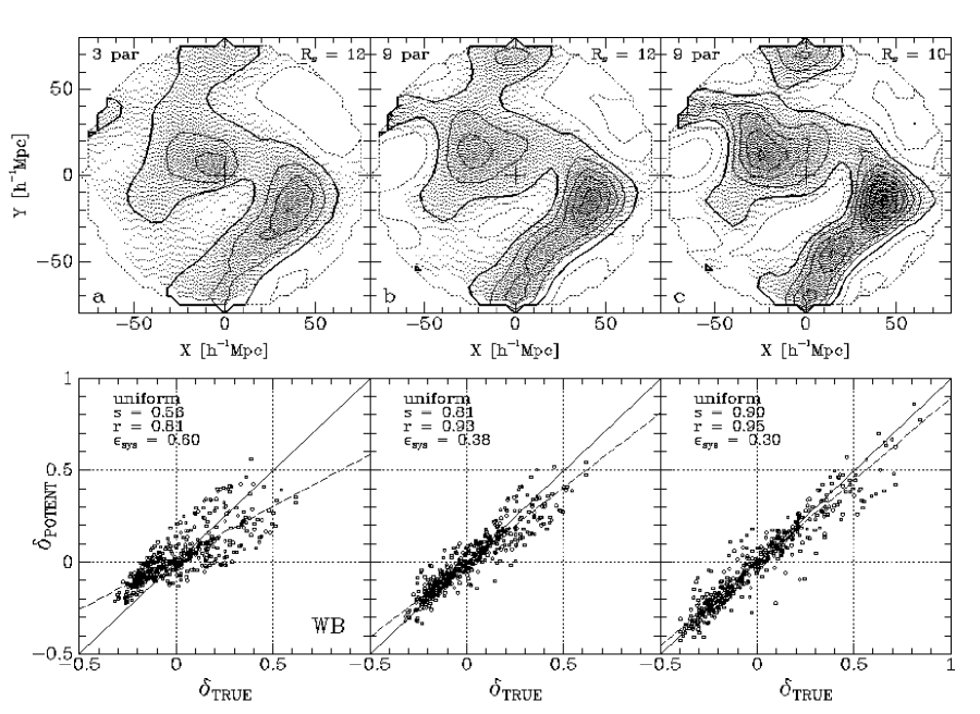
Figure 6: Window bias in the recovered density field. Mock unperturbed and uniformly sampled data as in Figure 5. Top: maps in the Supergalactic plane, to be compared to the true fields with the corresponding smoothings (Figure 4, left panels). Contours are as in Figure 2. Bottom: point-by-point comparison with the true smoothed density field inside a sphere of radius $40\,h^{-1}{\rm Mpc}$. Error statistics are marked. (a) bulk-velocity fit with 3 parameters, G12. (b) 9-parameter fit, G12. (c) 9-parameter fit, G10.

The WB can be reduced by introducing shear into the local model velocity field,

$$\kern-0.24994pt\hbox{$v$}\kern-5.20601pt\kern 0.50003pt\hbox{$v$}\kern-5.20601pt\kern-0.24994pt\raise 0.43304pt\hbox{$v$}(\kern-0.24994pt\hbox{$x$}\kern-5.71527pt\kern 0.50003pt\hbox{$x$}\kern-5.71527pt\kern-0.24994pt\raise 0.43304pt\hbox{$x$})=\kern-0.24994pt\hbox{$B$}\kern-8.0868pt\kern 0.50003pt\hbox{$B$}\kern-8.0868pt\kern-0.24994pt\raise 0.43304pt\hbox{$B$}+\bar{\bar{\kern-0.24994pt\hbox{$L$}\kern-6.80557pt\kern 0.50003pt\hbox{$L$}\kern-6.80557pt\kern-0.24994pt\raise 0.43304pt\hbox{$L$}}}\cdot(\kern-0.24994pt\hbox{$x$}\kern-5.71527pt\kern 0.50003pt\hbox{$x$}\kern-5.71527pt\kern-0.24994pt\raise 0.43304pt\hbox{$x$}-\kern-0.24994pt\hbox{$x$}\kern-5.71527pt\kern 0.50003pt\hbox{$x$}\kern-5.71527pt\kern-0.24994pt\raise 0.43304pt\hbox{$x$}_{c})\ ,$$ (20)

with $\bar{\bar{\kern-0.24994pt\hbox{$L$}\kern-6.80557pt\kern 0.50003pt\hbox{$L$}\kern-6.80557pt\kern-0.24994pt\raise 0.43304pt\hbox{$L$}}}$ a symmetric tensor, which ensures local irrotationality. The zeroth-order, bulk-velocity model of 3 parameters is thus extended into a first-order velocity model of 9 parameters. The additional free components tend to “absorb” most of the bias, leaving the value of the model velocity at the window center, $\kern-0.24994pt\hbox{$v$}\kern-5.20601pt\kern 0.50003pt\hbox{$v$}\kern-5.20601pt\kern-0.24994pt\raise 0.43304pt\hbox{$v$}(\kern-0.24994pt\hbox{$x$}\kern-5.71527pt\kern 0.50003pt\hbox{$x$}\kern-5.71527pt\kern-0.24994pt\raise 0.43304pt\hbox{$x$}_{c})=\kern-0.24994pt\hbox{$B$}\kern-8.0868pt\kern 0.50003pt\hbox{$B$}\kern-8.0868pt\kern-0.24994pt\raise 0.43304pt\hbox{$B$}$, less biased.

Figure 5 (right panels) and Figure 6 (middle panels) demonstrate the improvement in the WB when the 9-parameter model is used. The bias in the velocity field is reduced by about a factor of two, the global bias in the density field is improved to $s=0.81$, and the local bias is much improved to $r=0.93$, such that the total systematic error in density is down to $\epsilon_{\rm sys}=0.38$. Adding an additional quadratic term to the model turns out not to lead to a significant further improvement. This means that, for the current data, one has to live with the level of WB remaining in the 9-parameter fit, which, for G12 smoothing, is still at the level of $-150\,{\rm km}\,{\rm s}^{-1}$ at the worst point near the GA.

Figures 5 and 6 demonstrate that the WB can also be reduced by reducing the window size. With G10 smoothing, the global bias in the density field is significantly improved to $s=0.90$, while the local bias is slightly improved to $r=0.95$, yielding together $\epsilon_{\rm sys}=0.30$ (Figure 6, right). A window significantly smaller than G10 is impractical with the current data; sparse sampling and large distance errors would limit the reconstruction to the very local neighborhood of Virgo and the LG.

Even for G12 smoothing, sampling and distance errors restrict use of the 9-parameter model. The danger of a high-order model is that it tends to pick up undesired small-scale noise — a problem that becomes severe at large distances, where distance errors are large. Furthermore, the poor sampling at large distances may make it difficult to find enough data points ($>9$) within the effective volume of the window to constrain a 9 parameter model. Fortunately, at these large distances ($r\gg R_{\rm s}$) the WB decreases independently of the sampling and errors, so one can return there to the simple local bulk-velocity fit. Based on experimenting with the mock catalogs, we find the optimal procedure to be a 9-parameter fit out to $r=40\,h^{-1}{\rm Mpc}$, a 3-parameter fit beyond $60\,h^{-1}{\rm Mpc}$, and a smooth transition region between these radii where we adopt a linear weighted mean of the two kinds of fit, smoothly varying from one to the other.

6.2 Sampling-Gradient Bias

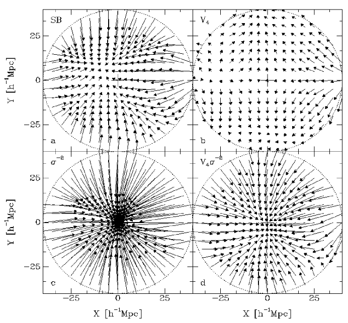
Figure 7: The origin of sampling-gradient bias. The displacements of the centers of mass of galaxies in a $12\,h^{-1}{\rm Mpc}$ Gaussian window from the window centers. The object positions and weights are from the Mark III catalog. Shown is the inner Supergalactic plane out to a distance of $40\,h^{-1}{\rm Mpc}$. (a) Unweighted, refering to the original SB. (b) Volume-weighted by $V_{4}$, to minimize SB. (c) Error-weighted by $\sigma^{-2}$, for optimal treatment of random errors. (d) A compromise: weighted by both volume and errors.

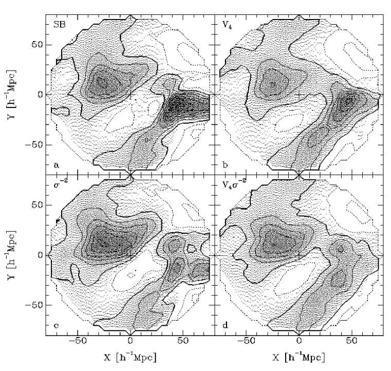
Figure 8: Sampling-gradient bias in the recovered density field in the Supergalactic plane. The input data are the true high-resolution radial velocities of the simulation, sampled non-uniformly at positions that mimic the spatial distribution of objects in the Mark III catalog. Contours are as in Figure 2. The four panels are as in Figure 7.

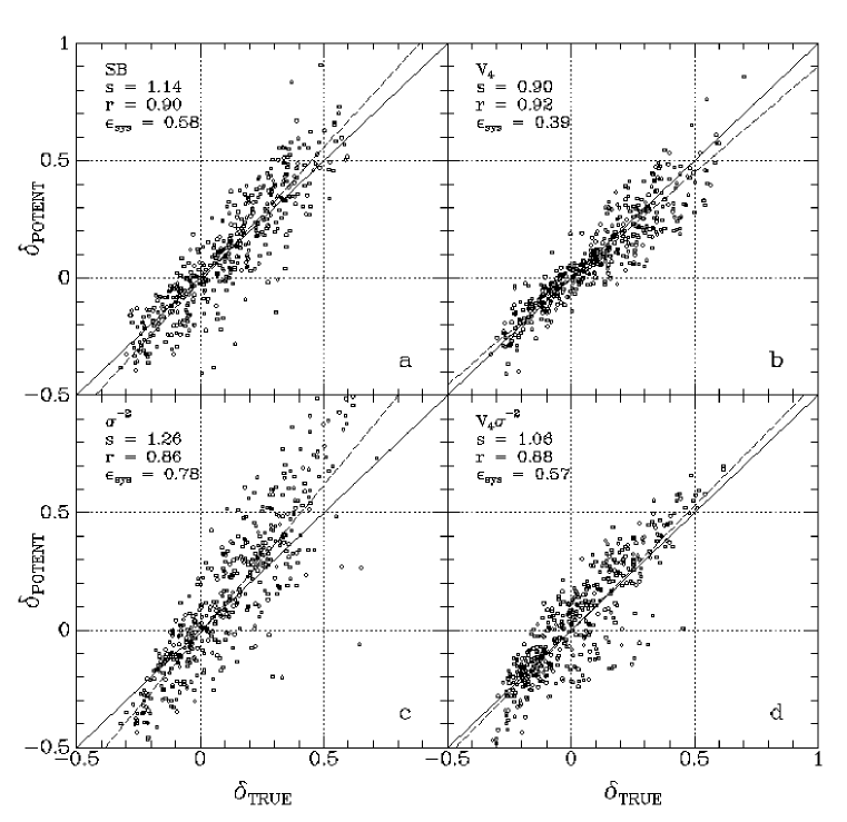
Figure 9: Sampling-gradient bias inside a sphere of radius $40\,h^{-1}{\rm Mpc}$. Mock unperturbed and non-uniformly sampled data as in Figure 8. The recovered density field is compared to the true G12 field at the points of a cubic grid, and the statistics measuring the typical systematic errors are quoted. The four panels are as in Figure 7.

If the true velocity field is varying within the effective window, non-uniform sampling introduces a sampling-gradient bias (SB), which has been evaluated analytically in DBF. The smoothing is galaxy-weighted whereas the aim is equal-volume weighting. In other words, the smoothed velocity as computed so far really refers to the Gaussian-weighted center of mass of the galaxies instead of the geographical window center.

Figures 7, 8 and 9 address the SB. Figure 7 illustrates the origin of the effect in the Supergalactic plane by showing the projected displacements of the window-weighted centers of mass of the Mark III galaxies from the window centers (positioned at the points of a cubic grid of spacing $5\,h^{-1}{\rm Mpc}$). These displacements are responsible for SB once the velocity field is varying within the window. In order to isolate the effects of SB (and remaining WB) from the effects of random errors, the POTENT procedure with G12 smoothing is applied to each of 10 special mock catalogs that mimic the nonuniform sampling of the Mark III objects, but with the true, unperturbed distances and velocities of the simulation. In these mock catalogs, the random properties assigned to the galaxies affect only the selection, not the distances or velocities. Figure 8 shows maps of the average recovered density field in the Supergalactic plane, while Figure 9 compares this field to the true G12 field at grid points inside a sphere of radius $40\,h^{-1}{\rm Mpc}$.

Panels (a) in these three figures refer to the uncorrected bias in the case of a spherical G12 window with no additional weights. The displacements in Figure 7a are typically comparable to the radius of the Gaussian window, and they in general follow the large-scale sampling gradient towards the origin. The resulting density map in Figure 8a is distorted accordingly, with the peaks of GA and PP overestimated, especially near the ZoA. The local systematic error within $40\,h^{-1}{\rm Mpc}$, Figure 9a, is typically $\epsilon_{\rm sys}=0.58$.

To correct for SB, we wish to weight each object in equation (19) by the local volume that it “occupies”, $V_{i}$. A simple way to estimate $V_{i}$ (see DBF) is via the inverse of the local density at the object as estimated crudely by the cube of the distance $R_{n}$ to its n-th neighboring object, $V_{i}\!\propto\!R_{n}^{3}$. For the current sampling density we find best results with $n\sim 4$. Panels (b) in the three SB figures demonstrate the significant reduction in SB when the Gaussian window is weighted by $V_{4}$. The displacements of the centers of mass in Figure 7b are of order of only a few $\!\,h^{-1}{\rm Mpc}$, much smaller than in panel a. The density map in Figure 8b becomes much more similar to the true field, Figure 4 (left), than panel a. The typical systematic error in Figure 9b is only $\epsilon_{\rm sys}=0.39$, and the global systematic error, $s=0.90$, is reminiscent of the remaining WB, Figure 6b, bottom panel.

The volume weighting can be improved further at the expense of making it more elaborate. For example, one can assign cells from a fine grid to neighboring objects and weight each cell by the value of the window function at the cell position. In this fancier procedure, a given object is weighted differently for windows centered at different positions. In practice, in view of the much larger distance errors discussed below, the simple $R_{4}$ procedure is presently adequate, and there is not much gain in applying the more elaborate procedure (which may however prove useful for future, better sampled data).

The tentative conclusion for the current Mark III sample is that the $V_{4}$ volume-weighting procedure could successfully reduce SB to negligible levels within the region where at least a few objects reside in the effective central region of the window. This region typically extends out to $60\,h^{-1}{\rm Mpc}$ from the Local Group outside the Galactic Zone of Avoidance. However, we shall see next that the need to deal with random distance errors prevents an optimal SB correction.

The same $R_{n}(\kern-0.24994pt\hbox{$x$}\kern-5.71527pt\kern 0.50003pt\hbox{$x$}\kern-5.71527pt\kern-0.24994pt\raise 0.43304pt\hbox{$x$})$ field also serves later (§ 8.1) as a useful diagnostic flag for poorly sampled regions, and as a criterion for excluding such regions from quantitative analyses. The displacement of the weighted center of mass from the window center likewise serves as a complementary flag for regions of high SB.

6.3 Weighting by Random Distance Errors

Each of the systematic errors in the POTENT analysis can in principle be corrected in a satisfactory way. However, the dominant errors in our reconstruction are the random errors due to scatter in the distance indicators and measurement errors. The random errors are particularly large at large distances, where both the error per object is big and the sampling is sparse such that shot noise becomes a major factor.

The standard way to reduce the effect of this roughly Gaussian noise and obtain the most probable smoothed field would be to weight the contribution of each object inversely by the variance of its distance (velocity) measurement error, i.e., $W_{i}\!\propto\!\sigma_{i}^{-2}$. In Figure 10, we isolate the effect of random velocity errors on the G12-recovered density field from one special mock catalog, and demonstrate the improvement resulting from the straightforward error weighting by $\sigma^{-2}$. In this case, the sampled galaxies are distributed uniformly  at the points of a cubic grid of spacing $6\,h^{-1}{\rm Mpc}$ inside a sphere of radius $100\,h^{-1}{\rm Mpc}$, thus eliminating SB if no additional weighting is applied. Random Gaussian perturbations of rms $20\%$ of the distance are assigned to the redshifts rather than the distances, thus avoiding the Malmquist bias (and the additional SB) that would be introduced by perturbing the distances (see § 7 below). The sampling spacing is chosen to be similar to the mean spacing in the well-sampled regions of the Mark III catalog (e.g., within a sphere of radius $22.5\,h^{-1}{\rm Mpc}$ about the LG and in the GA region), such that the resulting effect of the random errors on the smoothed fields in the mock realization is characteristic of that in the well-sampled regions of the real data.

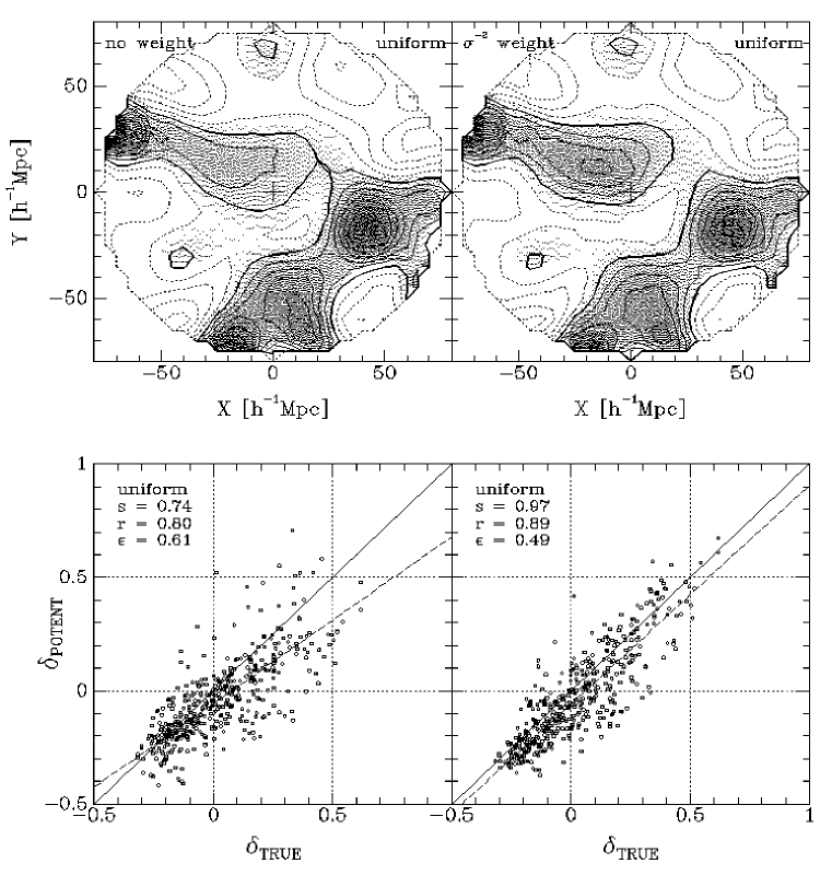
Figure 10: The effect of error weighting on one mock realization of perturbed velocities. The input sampling is uniform at the points of a grid of spacing $6\,h^{-1}{\rm Mpc}$, thus eliminating SB. The input velocities are at true distances, with the redshifts randomly perturbed instead of the distances, thus eliminating Malmquist bias. Top: maps in the Supergalactic plane of the recovered density field with and without error weighting, to be compared to the map of the true field (Figure 4, bottom left). Contours are as in Figure 2. Bottom: corresponding point-by-point comparisons of the recovered fields with the true density field of the simulation inside a sphere of radius $40\,h^{-1}{\rm Mpc}$. Error statistics are quoted.

The density maps of Figure 10 are to be compared to the true G12 field (Figure 4, bottom left or Figure 15a, below). With no error weighting, the GA density peak is underestimated and so is the depth of the local void, while the PP density peak is overestimated. The error weighting improves all three effects. The mean field recovered with error weighting still deviates from the true field because the input is after all severely perturbed, the sampling is not dense enough to eliminate shot noise, and the error weighting itself introduces sampling-gradient bias (that was absent in the unweighted recovery). A point-by-point comparison of the recovered and true fields is shown inside a sphere of radius $40\,h^{-1}{\rm Mpc}$. The statistics quoted refer in this case to the random errors only (when no weighting is applied, left panels) plus the artificial SB that is introduced by the $\sigma^{-2}$ weighting (right panels). With weighting, the regression slope drastically improves from $s=0.74$ to $0.97$, the local scatter improves from $r=0.80$ to $0.89$, and the total relative error is down from $\epsilon_{\rm tot}=0.61$ to $0.49$. We conclude, in this case of uniform sampling and random velocity errors only, that the error weighting leads to a significant improvement in the recovery.

Unfortunately, in the real case of non-uniform sampling, the error weighting somewhat spoils the volume weighting that has been carefully designed to minimize the sampling-gradient bias. The SB introduced by the $\sigma^{-2}$ weighting alone (without $V_{4}$ weighting) is shown in panels (c) of Figures 7-9 (which address the SB without random errors). In particular, the $\sigma^{-2}$ weighting tends to strongly bias the smoothed velocity towards the velocities in those parts of each window that are closer to the LG, where the errors are smaller and the sampling is typically denser. It may also bias the results towards the velocities of nearby clusters that may have small errors even if they lie relatively far from the central region of the window. The peaks in the density map of Figure 8c are too high and distorted, and the statistical measures show large global and local biases ($s=1.26$, $r=0.86$) with a total systematic error of $\epsilon_{\rm sys}=0.78$.

The standard compromise adopted here (as in BDFDB) is to weight simultaneously by the volume weights and  the inverse square of the random distance errors. Panels (d) of Figures 7-9 show the SB resulting in this case. With $\epsilon_{\rm sys}=0.57$, the bias is larger than in the case of weighting by $V_{4}$ alone, and is only slightly better than the raw SB bias with no weighting at all. However, given the requirement imposed by the random errors to weight by $\sigma^{-2}$, the combined weighting is a reasonable compromise. Thus, the value of the adopted window function at the position of object $i$ about the window center $\kern-0.24994pt\hbox{$x$}\kern-5.71527pt\kern 0.50003pt\hbox{$x$}\kern-5.71527pt\kern-0.24994pt\raise 0.43304pt\hbox{$x$}_{c}$ is of the form

$$W(\kern-0.24994pt\hbox{$x$}\kern-5.71527pt\kern 0.50003pt\hbox{$x$}\kern-5.71527pt\kern-0.24994pt\raise 0.43304pt\hbox{$x$}_{i},\kern-0.24994pt\hbox{$x$}\kern-5.71527pt\kern 0.50003pt\hbox{$x$}\kern-5.71527pt\kern-0.24994pt\raise 0.43304pt\hbox{$x$}_{c})\propto V_{i}\,\sigma_{i}^{-2}\,\exp[-(\kern-0.24994pt\hbox{$x$}\kern-5.71527pt\kern 0.50003pt\hbox{$x$}\kern-5.71527pt\kern-0.24994pt\raise 0.43304pt\hbox{$x$}_{i}-\kern-0.24994pt\hbox{$x$}\kern-5.71527pt\kern 0.50003pt\hbox{$x$}\kern-5.71527pt\kern-0.24994pt\raise 0.43304pt\hbox{$x$}_{c})^{2}/2R_{\rm s}^{2}]\ ,$$ (21)

up to a normalization factor. By not allowing the $V_{i}$ values to differ from their mean value by more than a factor of five (say), the deviation of the smoothed velocity from the most likely signal given the noisy data is kept limited to a reasonable range, while the SB is still significantly reduced compared to the case of weighting by $\sigma_{i}^{-2}$ only.

Two additional comments regarding the error weighting are appropriate. First, as mentioned above, we try to keep the smoothing radius $R_{\rm s}$ constant throughout the volume for the purpose of statistical spatial uniformity that allows straightforward direct comparison with theoretical models or other data of uniform smoothing. However, if desired, one could easily vary $R_{\rm s}$ such that the random errors of the recovered fields are kept roughly at a constant level throughout the volume (DBF).

Second, the error weighting typically distorts the spherical window shape and reduces its effective volume, thus mimicking smoothing with higher resolution. This effect turns out to roughly compensate for other effects that cause over-smoothing, such as SB in empty regions (§ 8.2).

After introducing Malmquist bias in the next section, we will address in § 8 the errors of all sources combined.

7 MALMQUIST BIAS CORRECTION

The random scatter in the distance estimator is a source of distinct systematic biases in the inferred distances and peculiar velocities, which are generally termed “Malmquist bias” but should be carefully distinguished from each other as described below (e.g., Lynden-Bell et al. 1988; DBF; Willick 1994; 1998). We describe three different ways of correcting for Malmquist bias and compare the results. The Malmquist correction is actually applied to the peculiar-velocity data in a preliminary stage, before they are fed into the main POTENT analysis, but we discuss it only here, after discussing the rest of the method, because it is a complication that is relatively independent of the other steps of the POTENT procedure, and we prefer to test it with the full POTENT machinery in hand.

7.1 Forward TF Correction

The calibration of the “forward” TF relation $M_{\scriptscriptstyle\rm TF}(\eta)$ is affected by a calibration  bias (or selection  bias). An apparent magnitude limit in the selection of the sample used for calibration at a fixed true distance (e.g., in a cluster) tilts the forward TF regression line of $M$ on $\eta$ towards bright magnitudes $M$ at small $\eta$ values. This bias may extend to all values of $\eta$ when objects over a large range of distances are used for the calibration. This bias is inevitable when the dependent quantity (here $M$) is explicitly involved in the selection process, and it occurs to a certain extent even in the “inverse” TF relation $\eta_{\scriptscriptstyle\rm TF}(M)$ due to weak dependencies of selection on $\eta$. The calibration bias can be properly corrected once the selection function is known, as explained, e.g., in Willick et al. (1995), and we assume hereafter that the given Mark III TF parameters are unbiased (but see § 9.5).

Even after the selection bias in the TF calibration is properly corrected, the TF-inferred distance, $d$, and therefore the mean peculiar velocity at a given $d$, suffers from an inferred-distance bias, which we term hereafter “Malmquist” bias or “MB”.

This bias can be reduced by grouping, and corrected in a statistical way. We devote a separate paper (Eldar, Dekel & Willick 1999) to the issue of Malmquist-bias in inferred-distance space, both in forward and inverse TF analyses, where we describe in more detail our correction procedures and test them with realistic mock data based on N-body simulations. Only a brief summary is provided here.

Malmquist bias can be quantified as follows. If the magnitude $M$ is distributed normally for a given log-velocity parameter $\eta$, with standard deviation $\sigma_{m}$, then the TF-inferred distance $d$ of a galaxy at a true distance $r$ is distributed log-normally about $r$, with relative error $\Delta=(\ln 10/5)\sigma_{m}$. Given $d$, the expectation value of $r$ is (e.g., Willick 1998):

$$E(r|d)={\int_{0}^{\infty}rP(r|d){\rm d}r\over\int_{0}^{\infty}P(r|d){\rm d}r}={\int_{0}^{\infty}r^{3}n(r)\ {\rm exp}\left(-{[{\rm ln}(r/d)]^{2}\over 2\Delta^{2}}\right){\rm d}r\over\int_{0}^{\infty}r^{2}n(r)\ {\rm exp}\left(-{[{\rm ln}(r/d)]^{2}\over 2\Delta^{2}}\right){\rm d}r}\ ,$$ (22)

where $n(r)$ is the number density of galaxies in the underlying distribution from which the galaxies were selected for the catalog (using $m$ and $\eta$ alone). Strictly, $n(r)$ depends on the particular line of sight to each galaxy. The deviation of $E(r|d)$ from $d$ is the Malmquist bias.

The “homogeneous” part (HM) refers to a constant $n(r)$ and arises from the geometry of space — the inferred distance $d$ underestimates $r$ because it is more likely to have been scattered by errors from a larger true distance $r>d$ than from a smaller true distance $r<d$, because the corresponding volumes are proportional to $r^{2}$. Another contribution to the HM bias arises from the fact that the distribution of $d$ about $r$ is not symmetric (it is $\log d$ that is symmetric about $\log r$). Quantitatively, if $n\!=\!const$, then equation (22) reduces to

$$E(r|d)=d\,e^{3.5\Delta^{2}}\ .$$ (23)

If all objects have the same error, the inferred distances are simply multiplied by a constant factor, increasing the distance by, e.g., about 10% for $\Delta=0.17$. This is equivalent to a global change of the zero point $a$ of the forward TF relation, equation (2). Grouped objects have smaller errors, and their corrections are smaller. The HM bias has been corrected this way on a regular basis (e.g., in Lynden-Bell et al. 1988).

Fluctuations in $n(r)$ are responsible for the “inhomogeneous” Malmquist bias (IM), which is worse because it systematically enhances the amplitude of the inferred density perturbations (and, consequently, the inferred value of $\Omega$). If $n(r)$ is varying slowly in the range $\pm\Delta r$ about $r$, and if $\Delta\ll 1$, then equation (22) reduces to

$$E(r|d)=d\,\left[1+3.5\Delta^{2}+\Delta^{2}\left({d\ln n\over d\ln r}\right)_{r=d}\right]\ ,$$ (24)

explicitly showing the dependence on $\Delta$ and on the gradient of $n(r)$. To illustrate the origin of IM bias, consider a lump of galaxies at one point $r$ with zero true peculiar velocity, $u\!=\!0$. Their inferred distances are randomly scattered to the foreground and the background of $r$. With all galaxies having the same redshift $z=r$, the inferred values of $u$ on either side of $r$ mimic a spurious infall towards $r$, which is then interpreted by the dynamical analysis as an attractor with a spurious overdensity at $r$.

In the forward-TF Mark III data for POTENT analysis, the standard correction for IM bias consists of two steps. First, the galaxies are properly grouped to “objects” as discussed above (§ 2; Willick et al. 1996), reducing the distance error of each group of $N$ members to $\Delta/\sqrt{N}$ and thus significantly weakening the bias. The noisy inferred distance of each object, $d$, is then replaced by $E(r|d)$ of equation (22), based on an assumed galaxy density profile $n(r)$ and with additional corrections for redshift limits in the data and for the grouping, as follows.

The practical uncertainty in the IM correction procedure is in the assumed function $n(r)$ along each line of sight. In principle, this could be obtained from the POTENT-recovered mass density itself through an iterative procedure under certain assumptions about how galaxies trace mass. However, the resolution provided by the Mark III data is not sufficient at large distances, where the IM bias is large and an accurate correction is needed. Instead, we approximate $n(r)$ from the high-resolution galaxy distribution in redshift surveys. For spirals, we use the galaxy density field in real space as recovered from the IRAS 1.2 Jy redshift survey, which is dominated by spirals. This recovery was done by Sigad et al. (1998) with G5 smoothing via a power-preserving filter assuming $\Omega=1$, no biasing $b=1$, and mildly non-linear corrections based on Nusser et al. (1991). For ellipticals and S0’s, we use a similar density field as recovered by Hudson (1995) from a survey of optical, mostly early-type galaxies. (This IM correction is similar but not identical to that published in Willick et al. 1997a.)

The redshift limits $z_{c}$, which are present in some of the Mark III datasets, are approximated as cutoffs in $n(r)$ at a given distance $r_{c}$. For most datasets, where the cutoff is beyond $8500\,{\rm km}\,{\rm s}^{-1}$, we adopt $r_{c}=z_{c}$. For the Aaronson et al. (1982) data, which are truncated at a heliocentric redshift $z_{c}=3000\,{\rm km}\,{\rm s}^{-1}$, we compute $r_{c}$ under the assumption of a constant bulk flow $B$$B$$B$ across the sampled volume, i.e., $r_{c}=z_{c}-\kern-0.24994pt\hbox{$B$}\kern-8.0868pt\kern 0.50003pt\hbox{$B$}\kern-8.0868pt\kern-0.24994pt\raise 0.43304pt\hbox{$B$}\cdot\hat{\kern-0.24994pt\hbox{$x$}\kern-5.71527pt\kern 0.50003pt\hbox{$x$}\kern-5.71527pt\kern-0.24994pt\raise 0.43304pt\hbox{$x$}}$ in the direction $\hat{\kern-0.24994pt\hbox{$x$}\kern-5.71527pt\kern 0.50003pt\hbox{$x$}\kern-5.71527pt\kern-0.24994pt\raise 0.43304pt\hbox{$x$}}$. Based on our results in § 10, we adopt for this correction a bulk flow of amplitude $350\,{\rm km}\,{\rm s}^{-1}$ in the direction $l=310^{\circ}$, $b=10^{\circ}$. (The actual bulk flow used in this MB correction has only a small effect on the measured bulk flow from the corrected data. Anyway, by using in the MB correction the same bulk flow as finally obtained from the corrected data, the correction is made self-consistent.)

When the data are grouped, the density profile $n(r)$ which enters the integrals in equation (22) has to be multiplied by another correction factor. In principle, the distances of all groups of a given richness, which have the same relative error, should be corrected using specifically just the number density of such groups. Because of the limited number of objects, we simplify the procedure and distinguish only between grouped and ungrouped galaxies. The density profile that enters equation (22) for ungrouped galaxies is multiplied by $f_{\rm ug}(r)$, the fraction of ungrouped galaxies in the vicinity of $r$ along the given line of sight. For groups, the number density is multiplied by $1-f_{\rm ug}(r)$. Because of the sparse sampling, we use for $f_{\rm ug}(r)$ the spherical average within each dataset. This is one source of inaccuracy in the correction.

7.2 Comparison to Inverse TF Correction in Inferred-Distance Space

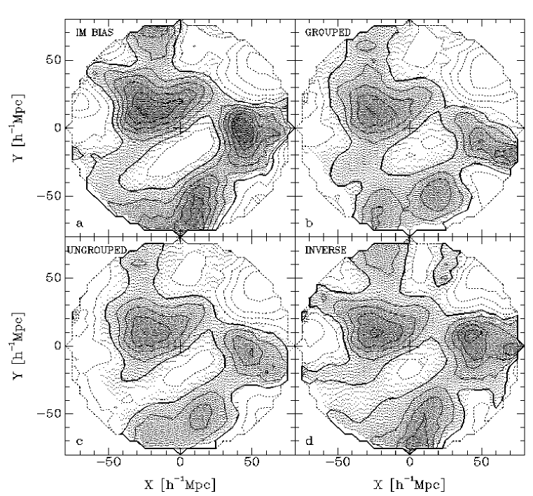
Figure 11: Malmquist bias corrections. Maps of POTENT G12 $\delta$ fields averaged over 10 random mock catalogs, corrected for homogeneous and inhomogeneous Malmquist bias in three different ways. The maps are to be compared to the true G12 field (Figure 4, bottom left). Contours are as in Figure 2. (a) Forward correction for HM bias only, (b) Forward IM-bias correction applied after grouping, (c) Forward IM-bias correction applied with no grouping, (d) Inverse IM-bias correction in inferred-distance space.

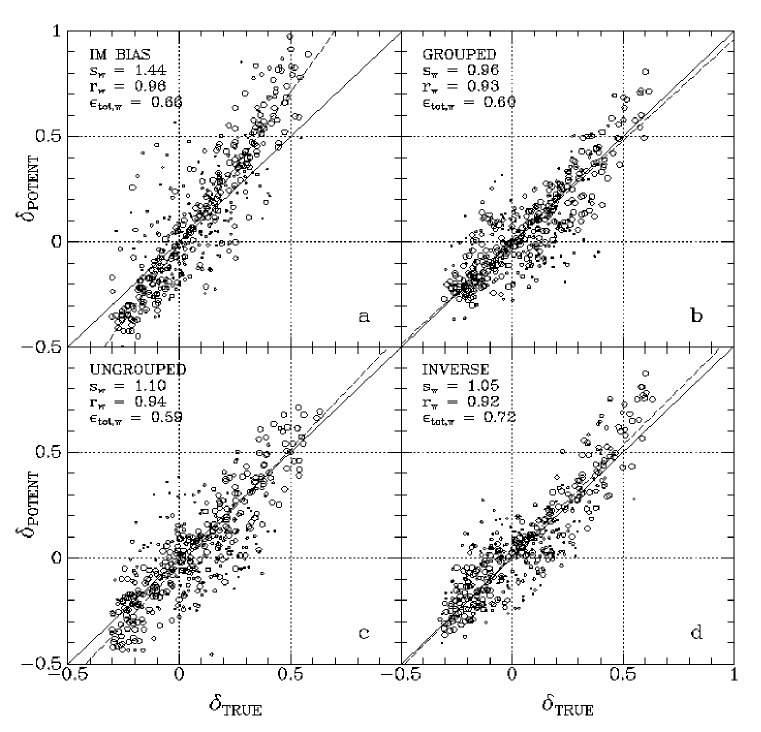
Figure 12: Malmquist bias corrections. Point-by-point comparisons of the average  G12 $\delta$ fields as recovered from 10 mock catalogs with the different correction procedures of Figure 11 and the true field. The area of each symbol is inversely proportional to the error $\sigma_{\delta}^{2}$ as determined by the dispersion over the random realizations (§ 8). The weighted regression lines are shown, and the corresponding weighted statistics are quoted (defined in § 4).

Distances, $d_{\rm inv}$, can alternatively be inferred via the inverse  TF relation between the log-velocity parameter $\eta$ and the magnitude $m$, namely,

$$\eta_{\scriptscriptstyle\rm TF}(M)=a_{\rm inv}-b_{\rm inv}M,\quad{\rm where}\quad M=m-5\log d_{\rm inv}\ ,$$ (25)

by identifying $\eta_{\scriptscriptstyle\rm TF}(M)$ with the observed $\eta$. The Malmquist bias is corrected in this case by Eldar, Dekel & Willick (1999) following the method proposed by Landy & Szalay (1992). Instead of the externally supplied density run $n(r)$, the sufficient input in this case is the number density of galaxies $\tilde{n}(d_{\rm inv})$, which is in principle derivable from the sample itself. Under the assumption that the selection is independent of $\eta$, the expectation value of the true distance $r$, given $d_{\rm inv}$, is

$$E(r|d_{\rm inv})=d_{\rm inv}\ e^{3.5\Delta_{\rm inv}^{2}}\ {\tilde{n}(d_{\rm inv}\,e^{\Delta_{\rm inv}^{2}})/\tilde{n}(d_{\rm inv})}\ ,$$ (26)

where $\Delta_{\rm inv}\equiv(\ln 10/5)\,\sigma_{\eta}/b_{\rm inv}$ is the relative error in $d_{\rm inv}$ (in which $\sigma_{\eta}$ is the scatter in the inverse TF relation), and is assumed to be small. In practice, the sparseness of the sample makes the derivation of $\tilde{n}(d_{\rm inv})$ non-trivial, and this is the main source of error in this MB correction procedure.

Figures 11 and 12 demonstrate, in maps and point-by-point comparisons with the true $\delta$ field, the success of the full POTENT reconstruction including the full Malmquist-bias correction done in three different ways: a forward correction via equation (22) with a preliminary grouping procedure, a forward correction without grouping, and an inverse correction via equation (26). Shown as a reference is the case where no special correction was applied beyond the simple forward correction for HM bias. The input data are the fully perturbed mock catalogs, and shown in the figure are the average fields over 10 realizations. All the IM-bias corrections turn out to be reasonably good, with a global bias of only a few percent ranging from $s_{\rm w}=0.95$ to $1.10$, and a local bias measured by $r_{\rm w}=0.92$ to $0.94$. (Note that once the fully perturbed mock catalogs are used we started quoting the “weighted” statistics, as defined at the end of § 4 and using the error weights $\sigma_{\delta}=\sigma_{\rm ran}$ specified in § 8.1 below; this is motivated by the assertion that subsequent analyses using POTENT output may use similar weights.) The total error is at the level of $\sim 60\%$ and $70\%$ of $\sigma_{\scriptscriptstyle\rm T}$ for the forward corrections and the inverse correction respectively. The “grouped” correction seems to be overall the best in terms of these statistics, but the differences in the quality of the reconstructions are small. In fact, the ranking of the methods should be different in different regions, depending on the sampling within each data set and on the true field itself. In § 9.4 below, Figure 24, we show a similar comparison of the three MB correction methods as applied to the real data. It is important to realize that the effect of the IM correction of the grouped Mark III data on the resultant density fluctuation with G12 smoothing is less than 20% even at the highest peaks. The bottom line is that the correction procedure reduces any remaining effects of Malmquist bias to the level of a few percent in the density field. The similarity between the results based on the different correction methods confirms the validity of our M-bias correction procedures.

It is worth mentioning that, in principle, Malmquist bias can be avoided altogether by performing the inverse TF analysis in redshift space using a parametric model for the velocity field (the “Schechter” method, e.g., Davis, Nusser & Willick 1996; Blumenthal, Yahil & Dekel 1999). However, this is done at the expense of a more complicated procedure, it involves other subtle biases, and it is based on a variable effective smoothing which does not straightforwardly provide a uniform reconstruction in real space.

8 REMAINING ERRORS IN POTENT

Having addressed the main sources of errors in POTENT one by one and having tried to minimize their effects on the recovered fields, we conclude the discussion of the method by evaluating its performance under realistic conditions, in which all the different sources of error are present simultaneously. In this section we use the fully perturbed mock catalogs described in § 3. Error flags are used to define standard “reference volumes” within which the quantitative evaluation is pursued. In the following text and figures we refer mostly to the “weighted” version of the evaluation statistics (§ 4 and below), but we list both the unweighted and weighted statistics in Tables 2 and 3.

8.1 Reference Volumes

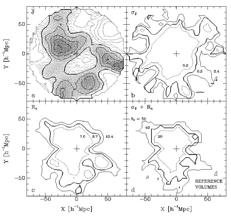
Figure 13: Reference volumes defined by errors in the Supergalactic plane. The maps are derived from G12 POTENT reconstructions of 10 mock catalogs. (a) The average $\delta$ field in the mock catalogs. Contours are as in Figure 2. (b) The standard deviation of the 10 $\delta$ fields. Contours from inside out are for $\sigma_{\delta}=0.2$, 0.3 and 0.4. (c) The average $R_{4}$ field. Contours from inside out refer to $R_{4}=7.0$, $8.7$ and $10.4\,h^{-1}{\rm Mpc}$. (d) Combined contours, of the pairs $(\sigma_{\delta},\,R_{4})=(0.2,\,7.0),\ (0.3,\,8.7),\ (0.4,\,10.4)$, corresponding to our reference volumes with effective radii of $R_{\rm e}=30$, 40, and $50\,h^{-1}{\rm Mpc}$ respectively.

The errors in the recovered fields are assessed empirically from the 10 random-realization mock catalogs, as explained in § 4. These are the mock catalogs described in § 3, which fully mimic the sampling and perturbed distances in the Mark III catalog. POTENT is applied to each of the mock catalogs, and the error at each grid point is the rms value over the realizations of $\delta$ there, either about their average ($\sigma_{\rm ran}$) or about the true density field ($\sigma_{\rm tot}$). In the present paper, we denote by $\sigma_{\delta}$ the $\sigma_{\rm ran}$ of the density field. The velocity error $\sigma_{v}$ can be computed similarly, component by component. This error estimate based on mock catalogs from simulations replaces the error estimate of DBF, which was based on a series of perturbed realizations of the real data. The new procedure avoids an artificial Malmquist-like bias that was problematic in the old procedure (see discussion in Dekel et al. 1993), and it includes the shot noise due to discrete sampling.

As an additional criterion for the quality of the reconstruction at each grid point, we use the same “emptiness” parameter $R_{4}$ used for volume weighting (§ 6.2), which also serves as a crude measure of sampling-gradient bias. The error flags $R_{4}$ and $\sigma_{\delta}$ are not independent everywhere; they can be either correlated or anti-correlated in different places. We find the correlation coefficient of $R_{4}$ and $\sigma_{\delta}$ inside spheres of radii $40$ and $80\,h^{-1}{\rm Mpc}$ to be $r=0.50$ and $0.46$ respectively (where $r=0$ refers to no correlation). As an example of a local anti-correlation between these error flags, consider empty regions such as the ZoA, in which the data weighted by the window function may be dominated by the velocities of many objects outside the central region of the window. The derived smoothed velocity in the empty region can thus be quite stable to random variations in these many inputs, despite the fact that hardly any local information is provided. In this case, the sampling bias introduces additional smoothing, which causes $\sigma_{\delta}$ to be artificially small. This provides additional motivation for using $R_{4}$ as a second criterion for an a priori evaluation of the quality of the reconstruction at a given point.

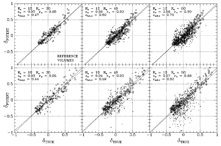
Figure 14: Biases in different reference volumes. Average reconstructed $\delta$ fields from 10 mock catalogs are compared to the true field of the simulation point by point inside reference volumes of effective radii $R_{\rm e}=30$, 40 and $50\,h^{-1}{\rm Mpc}$. The smoothing scale is $R_{\rm s}=12$ or $10\,h^{-1}{\rm Mpc}$. Symbols are as in Figure 12. The weighted regression line is shown, and the corresponding weighted statistics are quoted. The total error is the sum in quadrature of the systematic and random errors (equation (13)).

Figure 13 shows maps in the Supergalactic plane of $\sigma_{\delta}$ (G12) and $R_{4}$, and a map of boundaries defined by pairs of values: $\sigma_{\delta}<\sigma_{\delta,{\rm max}}$ and $R_{4}<R_{4,{\rm max}}$. We define the “effective radius” of the volume encompassed by a given error surface as the radius of a sphere that has the same volume. For example, with $\sigma_{\delta,{\rm max}}=0.3$ and $R_{4,{\rm max}}=8.7\,h^{-1}{\rm Mpc}$, the effective radius is $R_{\rm e}=40\,h^{-1}{\rm Mpc}$. High-quality reconstruction is limited to effective radii of order $40\,h^{-1}{\rm Mpc}$, while medium-quality reconstruction can extend out to $\sim 60\,h^{-1}{\rm Mpc}$ or more in certain directions, such as the parts of the GA that lie outside the ZoA.

Figure 14 shows the systematic errors, via point-by-point comparisons of the average reconstructed $\delta$ fields over the mock realizations and the true density field of the simulation. The comparison is made inside three different volumes of comparison, of effective radii $R_{\rm e}=30$, 40, and $50\,h^{-1}{\rm Mpc}$. The criteria are as in Figure 13. For the G10 smoothing, the error criteria are $(\sigma_{\delta},\,R_{4})=(0.25,\,7.5),\,(0.35,\,10.7)$ and $(0.45,\,13.5)$ for the same effective radii respectively. The global bias is consistently small in this range of smoothings and reference volumes, ranging from $s_{\rm w}=0.97$ to $0.93$. The local bias naturally increases as the volume becomes larger and the smoothing length becomes smaller. For both smoothings, the total error becomes larger than 70% of $\sigma_{\scriptscriptstyle\rm T}$ only near $R_{\rm e}=45\,h^{-1}{\rm Mpc}$ or beyond. Note in particular the large scatter of points with large errors in the $R_{\rm s}=10$, $R_{\rm e}=50$ case.

8.2 Error Analysis

We are now in a position to conclude the error analysis of POTENT based on the mock catalogs. Tables 2 and 3 summarize the performance of POTENT with mock data of gradually increasing complexity. In each case, the various measures of errors in the reconstructed mass-density field are given in comparison with the true density field, as defined in § 4. The statistics reported in Table 2 treat all the grid points within the reference volume equally, while the statistics reported in Table 3 weight the data at each grid point by the local random POTENT error there, $\sigma_{\delta}^{-2}$. These tables provide a full summary of the testing results. They refer to corresponding sections and figures, where appropriate.

The remaining systematic errors  after the optimization of POTENT are shown in Figures 15 and 16. In accordance with the tables, we show a sequence of POTENT output density fields in which the complexity of the mock input data drawn from the simulation grows gradually as follows:

• The input consists of the radial components of the true  G12  velocities on a spherical grid, as in § 5.3 (relevant only to Figure 16).

• The input is the true radial velocities sampled densely and uniformly  and then G12 smoothed by POTENT with 9 parameters nearby and 3 parameters at large radii. The result shows the remaining window bias (§ 6.1).

• The input of each of 10 realizations consists of the true radial velocities sampled at random, sparsely  and non-uniformly , mimicking the statistical properties of the Mark III sample. The average result shows the additional effect of sampling-gradient bias remaining after volume weighting by $V_{4}$ (§ 6.2).

• The input of each of 10 realizations consists of fully perturbed  positions and (therefore perturbed) radial velocities sampled at random to mimic Mark III, as described in § 3. The average result shows the additional systematic effect of random errors remaining after our correction for Malmquist bias (§ 7) and the additional weighting by $\sigma^{-2}$ (§ 6.3).

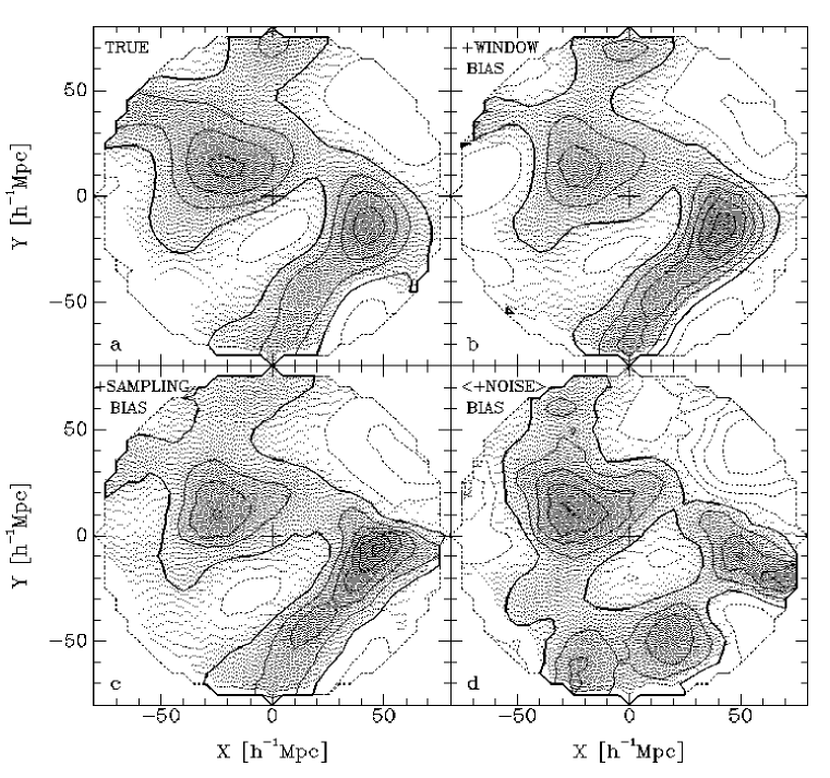
Figure 15: A summary of systematic errors in POTENT. Shown are maps of the G12 density fluctuation field $\delta$ in the Supergalactic plane of the mock catalogs. Contours are as in Figure 2. (a) The true field of the simulation (same as Figure 4, bottom-left panel). (b) The effect of window bias as shown by a POTENT reconstruction from noiseless radial velocities sampled uniformly at dense grid points of spacing $6\,h^{-1}{\rm Mpc}$, smoothed with an unmodified Gaussian window and using a 9-parameter fit (as in Figure 6b, § 6.1). (c) The effect of sparse and non-uniform sampling as demonstrated by the average field of 10 POTENT reconstructions from noiseless mock catalogs, with a window corrected for equal-volume weighting, $V_{4}$ (§ 6.2). (d) The total systematic error field, including the effect of distance errors, as shown by the average field of 10 POTENT reconstructions from noisy mock catalogs, corrected for Malmquist bias (§ 7), with additional $\sigma^{-2}$ weighting (§ 6.3).

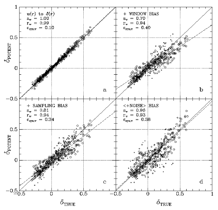
Figure 16: A Summary of systematic errors in POTENT. Shown are point-by-point comparisons of the G12 reconstructed density fields from the mock catalogs and the true density field of the simulation. The comparison is made at points of a cubic grid of spacing $5\,h^{-1}{\rm Mpc}$ within a sphere of radius $40\,h^{-1}{\rm Mpc}$. (a) POTENT reconstruction from perfect input of the exact radial components of the true G12 velocity field (same as Figure 4, bottom-right panel). Panels (b), (c) and (d) are the same as the corresponding panels of Figure 15; panels (c) and (d) refer to the average reconstructed fields of 10 noiseless and noisy mock catalogs respectively. Symbols, regression lines and statistics are as in Figure 12.

As the mock data evolve from the ideal case to the realistic noisy case, the quality of the reconstruction gradually deteriorates. The maps deviate steadily from the true map, and the local residuals in the scatter diagrams grow accordingly. The corresponding weighted correlation coefficients (defined in § 4) are $r_{\rm w}=0.99$, $0.94$, $0.94$, $0.93$. The fact that the only significant drop in $r_{\rm w}$ occurs between cases (a) and (b) indicates that the biases due to the non-uniform sampling and the random errors are well corrected while the remaining local bias is dominated by the window bias.

The global bias is characterized by $s_{\rm w}=1.00$, $0.70$, $0.81$, $0.96$ respectively. There is in fact a significant improvement after the introduction of non-uniform sampling and noise in the data due to the appropriate corrections in the smoothing scheme. This is due to the fact that the under-smoothing induced by the $V_{4}\sigma^{-2}$ weighting roughly compensates for the over-smoothing introduced by the window bias (as mentioned at the end of § 6.3). The final global bias of only $4\%$ (for the weighted fit within the reference volume) is very promising for further analysis involving linear regression (e.g., Sigad et al. 1998).

The random errors remain the dominant source of uncertainty. To illustrate their possible effects, we show in Figure 17 two noisy examples — the “best” and the “worst” G12 reconstructions among the 10 random noisy mock catalogs. The maps are to be compared to the true field (Figure 15a). Note that the reconstruction in the GA region is quite robust, while in PP it is more sensitive to the noise. The errors can be evaluated in these two cases by $s_{\rm w}=0.99$, $0.88$ and $r_{\rm w}=0.89$, $0.82$. These are the same statistics defined in § 4, but applied here to each of the two catalogs, not the average. The scatter in these individual reconstructions reflects both random and systematic errors and is therefore larger than the scatter in the mean reconstructed fields of Figure 14, which was dominated by the local systematic error at each grid point.

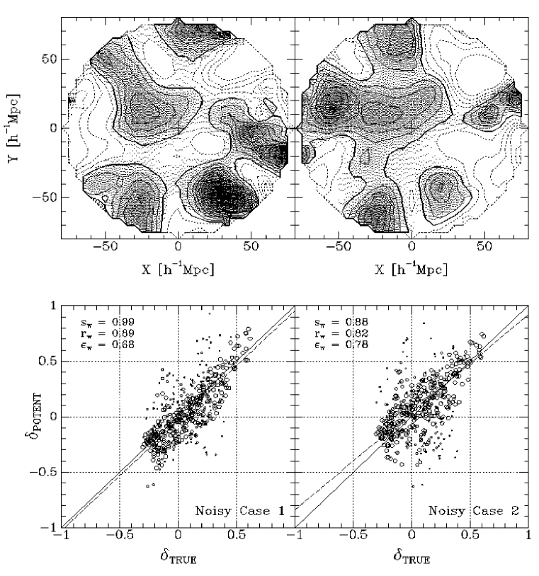
Figure 17: Two individual noisy realizations. Supergalactic maps of the reconstructed G12 $\delta$ fields from two individual mock catalogs and the corresponding point-by-point comparisons to the true field within $R_{\rm e}=40\,h^{-1}{\rm Mpc}$. Left: an example of a relatively good reconstruction. Right: an example of a relatively bad reconstruction. Contours and symbols are as in previous figures. Here, the statistics measure random errors in the individual realizations.

Supergalactic-plane maps of the error fields derived from the mock catalogs are shown in Figure 18. These error fields should be used when interpreting the POTENT density and velocity fields of the real data, such as the ones shown below (Figure 19). The error fields are crucial for any quantitative analysis using POTENT output.

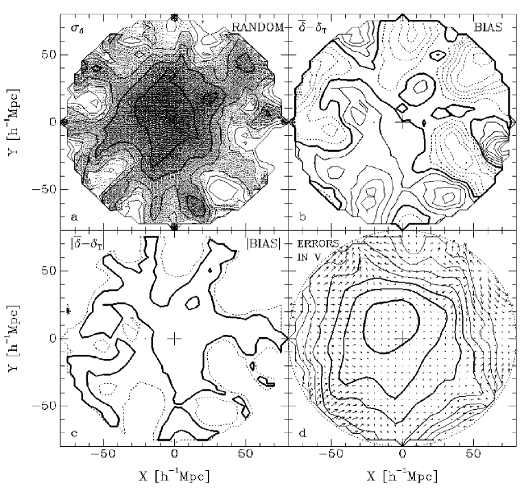
Figure 18: Error fields in the Supergalactic plane based on mock catalogs. (a) The random error in the density field, $\sigma_{\delta}$ (as in Figure 13b). Contours are 0.1, 0.2, 0.3, etc. (b) The systematic error in the density field, $\bar{\delta}-\delta_{\scriptscriptstyle\rm T}$. Contours are 0, $\pm 0.1$, $\pm 0.2$, etc. (solid and dashed curves for positive and negative bias respectively). (c) The absolute value of the systematic error in the density. Contours are 0.1, 0.2, etc. (d) Errors in the velocity field. The systematic-error field is marked by arrows. The random-error field $\sigma_{v}$ is mapped by contours of $100\,{\rm km}\,{\rm s}^{-1}$, $200\,{\rm km}\,{\rm s}^{-1}$, etc.

In order to evaluate one-point correlations between pairs of error fields of different types and other local quantities, we compute for each pair the linear correlation coefficient $r$ inside the reference volume of effective radius $40\,h^{-1}{\rm Mpc}$. For densities, the magnitudes of the random errors ($\sigma_{\delta}$) versus the systematic errors give $r=0.38$ — a positive but rather weak correlation. The magnitudes of the total error field ($\sigma_{\rm tot}$) versus the true density fluctuation field $|\delta_{\scriptscriptstyle\rm T}|$ show only a weak correlation, $r=0.08$ (with a slight correlation for the systematic component, $r=0.07$, and a slight anti-correlation for the random component, $r=-0.18$). Finally, the distance dependence of the errors in the recovered density field can be characterized by their correlation coefficients with distance: $r=0.83$, 0.40 and 0.77 for the magnitudes of the random, systematic and total errors respectively.

Our elaborate error analysis can be summarized by the following few numbers. Within the reference volume of effective radius $40\,h^{-1}{\rm Mpc}$, the rms systematic error in the local G12 density fluctuation field $\delta$ is $\pm 0.13$, and the corresponding random error is $\pm 0.18$, adding up in quadrature to a total (unweighted) error of $\pm 0.22$. The weighted total error in this volume is $\pm 0.15$.

9 POTENT RECONSTRUCTION FROM REAL DATA

We are now ready to apply POTENT to the real Mark III data. While showing the reconstruction of our cosmological neighborhood, we will also have additional opportunities to address some of the systematic errors discussed above.

The final POTENT Mark III maps of the G12 smoothed fields of projected three-dimensional peculiar velocity and of mass density fluctuations are presented in Figures 19 to 22. Figure 19 shows maps of the POTENT recovery in the Supergalactic plane. Figure 20 helps in visualizing the density field in the Supergalactic plane via a surface landscape plot in which height is proportional to the density fluctuation. Figure 21 adds the fields in two planes parallel to the Supergalactic plane, at $Z=-25$ and $+20\,h^{-1}{\rm Mpc}$. Finally, Figure 22 provides a three-dimensional view of the density fluctuation field via the surface of constant density fluctuation $\delta=0.4$. The density fluctuation shown in all these plots is computed assuming $\Omega\!=\!1$ in equation (18), but it can be easily generalized to any reasonable value of $\Omega$. Recall that the linear correction is simply a scaling by $f(\Omega)^{-1}$.

9.1 The Supergalactic Plane

The velocity map in Figure 19 shows a clear tendency for motion from right to left, in the general direction of the LG motion in the CMB frame (which is $L,B\!=\!139^{\circ},-31^{\circ}$ in Supergalactic coordinates). The bulk velocity within $60\,h^{-1}{\rm Mpc}$ is roughly $300-350\,{\rm km}\,{\rm s}^{-1}$ towards ($L,B\!\approx\!170^{\circ},-10^{\circ}$) (§ 10), but the flow is not coherent over the whole volume sampled, e.g., there are regions in front of PP (bottom right) and behind the GA (far left) where the $XY$ velocity components vanish, i.e., the streaming relative to the LG is opposite to the bulk flow direction. The velocity field shows local convergences and divergences which indicate strong density variations on scales about twice as large as the smoothing scale. The G12-smoothed velocity at the LG is $547\,{\rm km}\,{\rm s}^{-1}$ towards $(L,B)=(161^{\circ},-19^{\circ})$, compared to the unsmoothed LG motion relative to the CMB of $627\,{\rm km}\,{\rm s}^{-1}$ towards $(L,B)=(139^{\circ},-31^{\circ})$ (Lineweaver et al. 1996; Yahil et al. 1977)

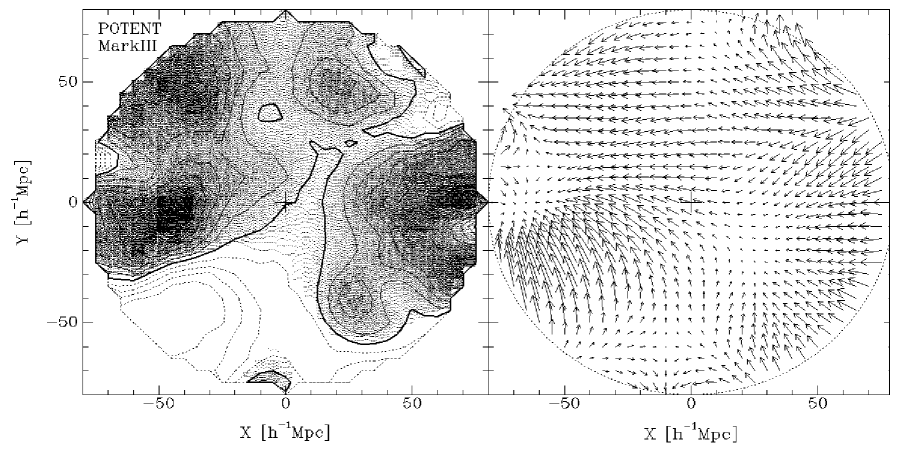
Figure 19: POTENT recovery of real data. The fluctuation fields of velocity and mass density in the Supergalactic plane as recovered by POTENT from the Mark III peculiar velocities with G12 smoothing. Left: As in previous density maps, the contour spacing is 0.2, the heavy contour marks $\delta=0$, and the dashed contours correspond to $\delta<0$. The grey scale is proportional to $\delta$. Right: The three-dimensional velocity field relative to the CMB frame is projected onto the Supergalactic plane. Distances and velocities are in $\!\,h^{-1}{\rm Mpc}$ or $100\,{\rm km}\,{\rm s}^{-1}$. The LG is at the center. The GA is on the left, PP on the right, and a large local void lies in between.

Figure 20: The POTENT density field in the Supergalactic plane out to $80\,h^{-1}{\rm Mpc}$, as in Fig 19, shown as landscape maps observed from two different directions. The height of the surface is proportional to $\delta$. Note the attractors GA and PP, and the extended void in between.

The Great Attractor (with G12 smoothing and $\Omega\!=\!1$) is a broad density ramp of maximum height $\delta\!=\!1.4\pm 0.3$ located near the Galactic plane $Y\!=\!0$ at $X\!\approx\!-40\,h^{-1}{\rm Mpc}$. The GA extends through the Hydra and Centaurus clusters towards Virgo near $(X,Y)\!\approx\!(0,10)$ (the “Local Supercluster”), towards Pavo–Indus–Telescopium (PIT) across the Galactic plane to the south ($X\!<\!0$ and $Y\!<\!0$), and towards the Shapley concentration behind the GA ($X\!<\!0,Y\!>\!0$). The structure at the top is related to the “Great Wall” of Coma, with $\delta\approx 0.6$. The Perseus–Pisces structure, which dominates the bottom-right quadrant, peaks near Perseus with $\delta\!=\!1.0\pm 0.4$. PP extends towards the Southern Galactic Hemisphere (Aquarius, Cetus), coinciding with the “Southern Wall” as seen in redshift surveys. Underdense regions separate the GA and PP, extending from bottom-left to top-right. The deepest region in the Supergalactic Plane, with $\delta\!=\!-0.8\pm 0.3$, roughly coincides with the galaxy void of Sculptor (Kauffman et al. 1991).

9.2 Outside the Supergalactic Plane

We have focused so far on the fields in the Supergalactic plane, where the structure is rich, featuring large attractors and big voids. However, the data and the analysis span the three-dimensional space about the LG, and in particular regions away from the Supergalactic plane. The two slices shown in Figure 21 above and below the Supergalactic plane demonstrate the continuity and extent of the two big structures, the GA and PP, and how the large void stretches between them. The bulk flow is seen in all three slices, which means that it is valid throughout most of the volume analyzed. The combined error contour of $R_{\rm e}=50\,h^{-1}{\rm Mpc}$ ($\sigma_{\delta}<0.4$ and $R_{4}<10.4\,h^{-1}{\rm Mpc}$) encompasses parts of the GA and PP, but it excludes the parts of these structures that lie near the ZoA. The big streams on the right beyond PP are clearly noise features.

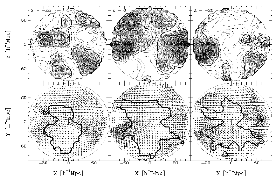
Figure 21: Same as Figure 19 but for two additional planes parallel to the Supergalactic plane, at $Z=-25$ and $+20\,h^{-1}{\rm Mpc}$. The heavy contours on top of the velocity fields are cuts through the surface $\sigma_{\delta}<0.4$ and $R_{4}<10.4\,h^{-1}{\rm Mpc}$, which has an effective radius of $50\,h^{-1}{\rm Mpc}$.

The three-dimensional structure in the whole volume is also illustrated in Figure 22, which shows the surfaces of $\delta=+0.4$. The GA and PP extend dramatically into the two sides of the Supergalactic plane and so does the big void between them. While the GA appears to be a coherent big structure, PP develops a more complex structure outside the Supergalactic plane and connects to other super-structures.

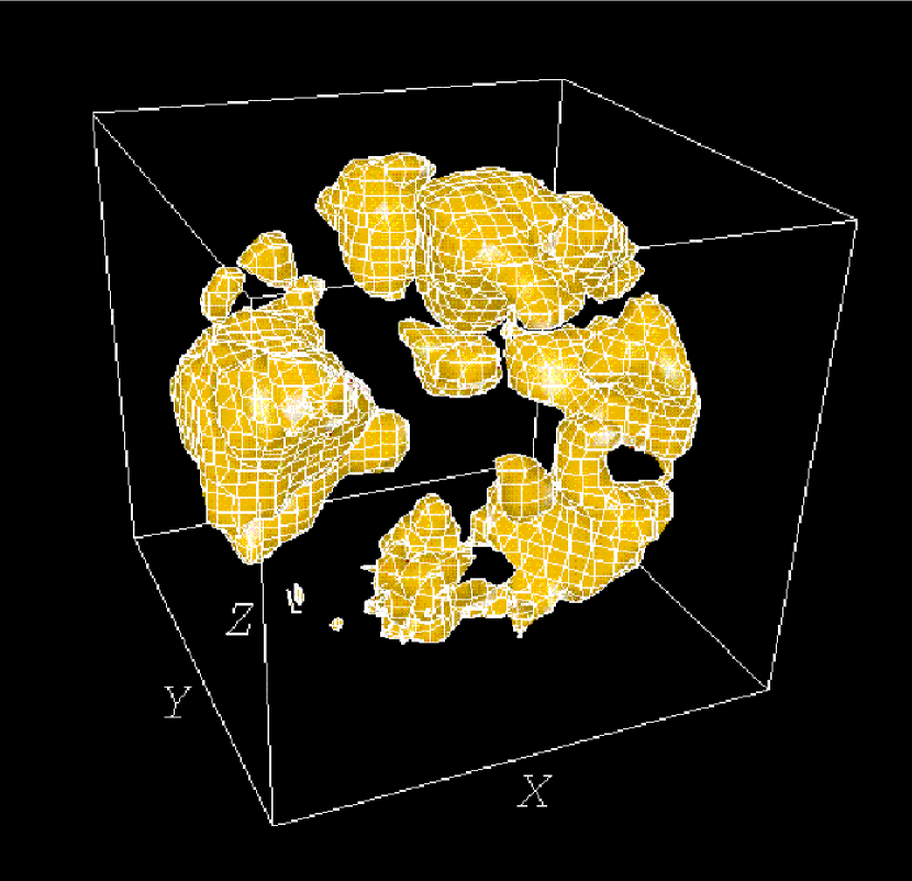
Figure 22: The POTENT G12 $\delta$ field in three dimensions. Shown is the surface $\delta=+0.4$. The box marks the Supergalactic coordinates $X,Y,Z$; the Supergalactic plane is the equatorial plane $Z=0$ and the LG is at the center of the cube. The GA is the big structure on the left and PP is the big complex structure extending above and below the Supergalactic plane on the right, with the big void in between.

9.3 Issues in Local Cosmography

Following are a few comments about issues of interest in the local cosmography.

One can still find in the literature statements questioning the existence of the GA (e.g., Rowan-Robinson 1993), which simply reflect ambiguous definitions for this entity. A GA clearly exists in the sense that a dominant feature in the local peculiar-velocity field is a coherent convergence, centered near $X\!\approx\!-40$. Whether or not the associated density peak has an exact counterpart in the galaxy distribution is another question. The GA is ambiguous only in the sense that the correlation observed between the mass density inferred from the velocities and the galaxy density in redshift surveys, though generally good, is not perfect (e.g., Sigad et al. 1998). This might reflect underestimated errors in the analyses, a nontrivial biasing relation between galaxies and mass, and/or incomplete coverage of the ZoA region by existing redshift surveys (see below).

The GA was originally discovered by Lynden-Bell et al. (1988) from the velocities of elliptical and S0 galaxies. Kolatt & Dekel (1994) found that the flows of spiral galaxies and early-type galaxies are consistent with each other, but Mathewson, Ford & Buchhorn (1992) expressed some doubts concerning the GA convergence in their spiral data. However, these data now dominate the Mark III data in that region. Figure 23 shows Supergalactic-plane maps of the POTENT velocity and density fields derived from spirals only. Comparison to the fields recovered from all the data, Figure 19, shows only minor differences. The GA and the other main features in our cosmological neighborhood are clearly present in a consistent way in the velocities of the tracers of all types.

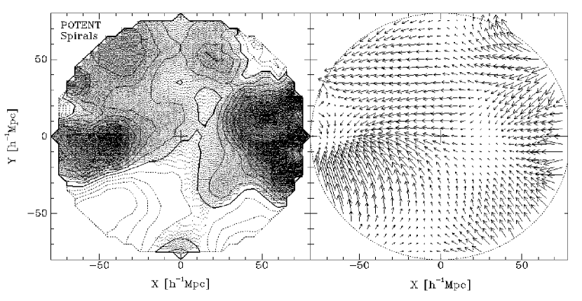
Figure 23: POTENT recovery from spirals only. The G12 fluctuation fields of velocity and mass density in the Supergalactic plane as recovered by POTENT from the Mark III peculiar velocities of spirals only. Compare to Figure 19.

It is also now possible to correct another misimpression as to the amplitude of the local GA inflow. Lynden-Bell et al. (1988) originally modeled the entire flow pattern within $40\,h^{-1}{\rm Mpc}$ of the LG as a spherical inflow onto an at-rest GA. The amplitude of this flow at the LG was $\sim 500\,{\rm km}\,{\rm s}^{-1}$, indicating a rather high mass for the GA. The analysis below (§ 10, Figure 27) decomposes the velocity field into its locally produced, divergent part and an externally produced, tidal part. It is seen there that only about half of the GA velocity is due to the GA and the local distribution of mass. Thus, very crudely, the mass excess associated with the GA should be only about half of that envisioned by Lynden-Bell et al.

Other debated cosmographic issues in the Supergalactic plane, are the nature of the flow behind the GA and the velocity of PP relative to the LG. The current POTENT analysis indicates that, although there are signs of a relative local backflow towards the GA center, the flow behind the GA in the CMB frame is dominated by a continuing outflow, roughly towards the Shapley concentration (see § 10 below). The region between the LG and PP shows small CMB velocities, namely, a velocity of recession away from the LG, but the central regions of PP seem to be roughly at rest relative to the LG. The back side of PP appears to be flowing towards PP, as expected, and is approaching the LG. However, the flows beyond the GA and PP are only marginally detected by the current data and POTENT analysis, at the $\sim 1.5\sigma$ level in terms of the random uncertainty. Furthermore, the remaining freedom in the zero point of the distance indicators (see § 9.5 and § 11.1) permits adding a Hubble-like peculiar expansion velocity to the whole ensemble, which could balance the flows at the back of the GA and in PP. Thus, these issues remain partly debatable until settled by future data of better sampling in these outer regions.

To what extent should one believe the reconstruction in the Galactic Zone of Avoidance (ZoA), in which the sampling is very poor? The velocities observed at medium Galactic latitudes on the two sides of the ZoA are used as probes of the mass in the ZoA. The interpolation is based on the assumed irrotationality, where the recovered transverse components allow a reconstruction of the mass-density. However, while the sampling-gradient bias can be corrected where the width of the ZoA is smaller than the smoothing length, the result could be severely biased in places where the unsampled region is larger. With G12 smoothing in the Mark III data, the interpolation is suspect of being severely biased in $\sim\!50\%$ of the ZoA at $r\!=\!40\,h^{-1}{\rm Mpc}$ (where $R_{4}\!>R_{\rm s}$), but the interpolation is fairly reliable, for example, in the closer and highly populated near side of the GA. Indeed, a deep survey of optical galaxies at low Galactic latitudes (Kraan-Korteweg et al. 1996) as well as data from the ROSAT X-ray satellite (Boehringer et al. 1996) revealed the very rich Abell cluster A3627 centered at $(l,b,z)\!=\!(325^{\circ},-7^{\circ},45\,h^{-1}{\rm Mpc})$, which is near the center of the broad peak of the GA as predicted earlier by POTENT from Mark III at $(320^{\circ},0^{\circ},40\,h^{-1}{\rm Mpc})$ (Kolatt, Dekel & Lahav 1995). This is in agreement with the theoretical expectation that rich clusters (originating from small-scale, high-amplitude peaks) prefer to form near the centers of larger superstructures (large-scale, low-amplitude peaks). In fact, it has become clear recently that the whole ZoA region between the Centaurus clusters and PIT contains enhanced galaxy density hidden behind heavy extinction, as high as 12 V magnitudes at $b=-1.5^{\circ}$ along the line connecting A3627 and Centaurus (Woudt 1998).

9.4 Sensitivity to Malmquist Bias: Forward vs. Inverse

Sensitivity to Malmquist bias is explored again in Figure 24, which shows maps in the Supergalactic plane of the reconstructed fields corrected in three different ways, as in Figure 11 of § 7.2 for the mock catalogs. Shown are Malmquist corrections in a forward TF analysis via equation (22) with (standsrd) and without a preliminary stage of grouping, and the result of an inverse TF analysis in inferred-distance space, where the correction is done via equation (26). (We do not have inverse-TF distances for the field ellipticals in Mark III, which constitute $\sim 16\%$ of the sample. In order to allow a comparison with the forward corrections of the whole sample, we added in panel (c) the forward-corrected elliptical distances to the inverse-corrected spiral distances.)

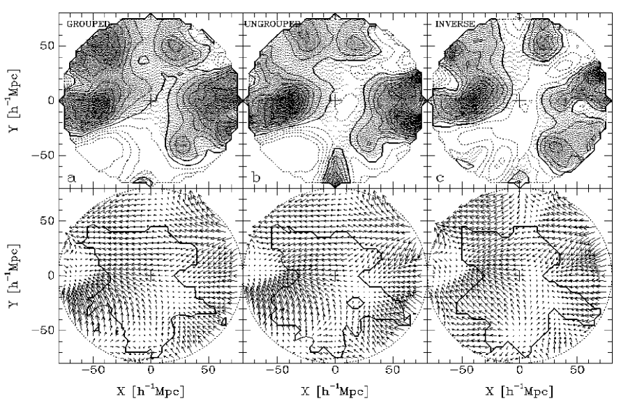
Figure 24: Three Malmquist-bias corrections of real data. Maps in the Supergalactic plane of the G12 mass-density and velocity fields from the Mark III data, corrected for Malmquist bias in three different ways as in Figure 11. Contours are as before. (a) forward correction after grouping, (b) forward correction with no grouping, (c) inverse correction in inferred-distance space. The error contours refer to an effective radius of $R_{\rm e}=50\,h^{-1}{\rm Mpc}$.

The maps are quite similar in their gross features. The GA has slightly higher density in the “ungrouped” correction compared to the “grouped” correction, while the “inverse” correction is intermediate between the two, but the difference at the highest peak is only $\sim 20\%$. There are differences in the fine details of PP, especially in the “inverse” correction compared to the “forward” cases, but the overall amplitude and shape within the error contour shown are not very sensitive to the grouping, and are not very different in the “inverse” case. The void between GA and PP is somewhat wider and deeper in the “inverse” and “ungrouped” cases compared to the “grouped” case. These differences in the fine details of the three maps can be interpreted as the typical residual error in the Malmquist-bias correction.

9.5 Sensitivity to TF Calibration

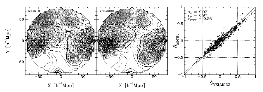
Figure 25: Alternative Zero-point Calibrations of Mark III. The G12 POTENT density field as reconstructed from the original Mark III data is compared with the density field as reconstructed from the alternative VM2 calibration of the same TF data. The comparison is made via maps in the Supergalactic plane and via a point-by-point comparison within a reference volume of effective radius $40\,h^{-1}{\rm Mpc}$. Contours, symbols, and statistics quoted are as before.

The relative  TF calibration of the various datasets that constitute the Mark III catalog suffers from dome uncertainty. The original relative calibration was done within the Mark III catalog itself based on galaxies that are common to more than one dataset. An alternative way to match the datasets is by requiring maximum agreement between the velocity field extracted from Mark III and the galaxy density field extracted from a whole-sky redshift survey, such as the IRAS 1.2 Jy catalog, under the assumption of a simple, linear biasing relation between the densities of galaxies and the underlying mass. A comparison of the corresponding density fields within $\sim 40\,h^{-1}{\rm Mpc}$ has indicated an acceptable goodness of fit using the original calibration of Mark III (Sigad et al. 1998). A similar conclusion has been obtained in the VELMOD high-resolution velocity-velocity comparison that was limited to an even smaller reference volume (Willick et al. 1997b). However, velocity-velocity comparisons of those two catalogs show a lower goodness of fit at larger radii (Davis, Nusser & Willick 1996; Willick & Strauss 1998). In particular, the VM2 analysis suggests a somewhat different relative TF calibration for the datasets of the Mark III catalog. The main proposed change boils down to the zero points of the datasets that cover the PP region. It works in the sense of reducing the distances by a multiplicative factor of 7–8%, thus reducing any inwards back-flow behind PP. (As far as the global zero point is concerned, in the original calibration we eventually reduced it by 3% in order to minimize the rms peculiar velocities of POTENT within $40-50\,h^{-1}{\rm Mpc}$, while no such correction is needed with the VM2 calibration.)

However, the mass density fluctuation is a function of the partial derivatives of the velocity field, which are only weakly sensitive to the TF zero point. Hence, changes of the proposed magnitude are expected to have only little effect on the density maps. This is confirmed in Figure 25, which compares the POTENT density fields as reconstructed from the original calibration and from the VM2 calibration of the same Mark III data. The differences are minor: in the revised calibration, the density of PP outside the ZoA is somewhat higher, and the void between the LG and PP is slightly wider. The small systematic difference within the reference volume of effective radius $40\,h^{-1}{\rm Mpc}$ is characterized by $s_{\rm w}=0.92$ and $r_{\rm w}=0.97$. These differences should serve as a crude estimate of the error associated with the relative zero-point calibration in the Mark III catalog; it is small compared to the other errors. The difference is larger in the bulk velocity at large radii (§ 10). A new systematic whole-sky survey of TF data in a shell between redshifts $4500$ and $7000\,{\rm km}\,{\rm s}^{-1}$ (Courteau et al. 1999, SHELLFLOW, hereafter SHF) should help reduce this uncertainty and thus allow a quantitative analysis in a larger reference volume.

10 BULK VELOCITY

The simplest statistic that can be used to characterize the peculiar-velocity field is the bulk velocity (in the CMB frame) within a given volume. The POTENT output allows a reliable measurement of the bulk velocity within top-hat concentric spheres about the Local Group out to radii of $50$-$60\,h^{-1}{\rm Mpc}$, beyond which the errors are large and uncertain (both for the Mark III data and for any other currently available TF whole-sky galaxy survey). One could alternatively compute the bulk velocity by a direct fit to the raw data of radial peculiar velocities of the individual galaxies, but the advantage of using the output of POTENT for this purpose is that it automatically provides equal-volume averaging and it avoids many of the biases associated with a direct fit. The disadvantage is that the $12\,h^{-1}{\rm Mpc}$-Gaussian smoothing significantly affects the resultant bulk flow out to radii of $20-30\,h^{-1}{\rm Mpc}$.

Random errors in the bulk velocities are determined by the rms scatter in the results obtained from the series of random noisy mock catalogs (§ 3). Systematic errors in the bulk velocity are determined by comparing the average over the mock catalogs with the true G12-smoothed bulk velocities in the simulations. In order to feed POTENT with mock data that have a bulk flow as large as the one observed (the large-scale bulk velocity in the simulation is artificially small because of the periodic boundary conditions), we added to the mock data an artificial component of bulk flow such that the total matches the flow obtained from the real data in a sphere of radius $60\,h^{-1}{\rm Mpc}$, namely $356\,{\rm km}\,{\rm s}^{-1}$ in the direction $(L,B)=(171^{\circ},-7^{\circ})$. Figure 26 shows the resultant bulk velocity as a function of radius $R$, both in shells and in spheres, for the original calibration of Mark III and for the proposed VM2 re-calibration.

Figure 26: The bulk velocity in the CMB frame in concentric shells or spheres of radius $R$ about the Local Group. It is derived by equal-volume vector weighting of the G12 uniform POTENT output. Shown is the magnitude of the bulk velocity and its three components in Supergalactic coordinates. Also shown are the random (error bars) and systematic (arrows) errors, derived from a series of mock realizations. Shown in comparison are the results from the original calibration of the Mark III TF data (solid) and from the proposed VM2 calibration (dashed).

Perhaps the most solid useful number from this analysis is the bulk flow relative to the CMB within the sphere of radius $50\,h^{-1}{\rm Mpc}$: $V_{\rm 50}=370\pm 110\,{\rm km}\,{\rm s}^{-1}$ towards $(L,B)=(165^{\circ},\,-10^{\circ})$ for the original calibration, and $V_{\rm 50}=305\pm 110\,{\rm km}\,{\rm s}^{-1}$ towards $(L,B)=(150^{\circ},\,0^{\circ})$ for the VM2 re-calibration of the same data. [The corresponding directions in Galactic coordinates are $(l,b)=(305^{\circ},\,14^{\circ})$ and $(314^{\circ},\,30^{\circ})$.] This bulk velocity is dominated by the negative $X$ component, which represents a coherent flow of much of the local region, including parts of PP, towards the GA and the Shapley Concentration behind the GA at roughly twice the distance. The error quoted includes both the random and systematic effects as determined from the mock catalogs. The magnitudes of these two components are comparable, as can be seen in Figure 26 where they are shown separately. The cosmic scatter, which is not included, could be of comparable magnitude to the quoted error, depending on the cosmological model assumed (including for example the power spectrum of fluctuations and the cosmological density parameter $\Omega$).

These results are quite similar to the results obtained by BDFDB from POTENT applied to the Mark II data, $V_{\rm 40}=388\pm 67\,{\rm km}\,{\rm s}^{-1}$ towards $(L,B)=(177^{\circ},\,-15^{\circ})$. Note that the errors are estimated more accurately in the current analysis, and the results are more reliable now out to $50$ or even $60\,h^{-1}{\rm Mpc}$. The current results from POTENT Mark III are also consistent with the results of Courteau et al. (1993) based on a direct likelihood analysis from preliminary Mark III radial velocities, in which a certain effort was made to approximate equal-volume weighting: $V_{\rm 60}=360\pm 40\,{\rm km}\,{\rm s}^{-1}$ towards $(L,B)=(177^{\circ},\,-23^{\circ})$. Note, again, that the errors are computed in different ways and they have different meanings.

For comparison, the bulk velocity within the sphere of radius $50\,h^{-1}{\rm Mpc}$ for the SFI catalog (Wegner et al. 1999, Haynes et al. 1999) analyzed via POTENT in a similar way is $V_{\rm 50}=310\pm 80\,{\rm km}\,{\rm s}^{-1}$ towards $(L,B)=(148^{\circ},\,-13^{\circ})$ (Eldar et al. 1999). A direct fit to the SFI radial velocities yields $V_{\rm 65}=200\pm 65\,{\rm km}\,{\rm s}^{-1}$ towards $(L,B)=(151^{\circ},\,-17^{\circ})$ (Giovanelli et al. 1998). The errors are estimated in yet a different way. These results all agree within the $1\sigma$ error. The VM2 calibration of Mark III also shows a bulk velocity similar to SFI shell by shell near $50\,h^{-1}{\rm Mpc}$ and beyond, and they are both smaller there than the bulk velocity from the original Mark III calibration. However, this is where the errors begin to become large and the bias corrections are uncertain in both catalogs.

Figure 27: A decomposition of the velocity field in the Supergalactic plane (a) into its “divergent” component, due to the mass fluctuations within $60\,h^{-1}{\rm Mpc}$ (b), and its “tidal” component, due to the mass outside this sphere (c). The residual left after subtracting the bulk from the tidal component includes quadrupole and higher moments in the tidal field (d). Velocities and distances are measured in $\,h^{-1}{\rm Mpc}$.

Where are the main sources of this bulk velocity? How much of it is contributed from the local distribution of mass, e.g., the GA, and how much is due to the mass distribution at larger distances? What are the main features of the velocity field on top of the bulk velocity? To begin to address these questions, we decompose the velocity field into two components: the “divergent” component arising from the mass fluctuation field within the sphere of radius $60\,h^{-1}{\rm Mpc}$ about the LG, and the “tidal” component arising from the mass distribution outside this sphere. The decomposition is performed as follows. First, the “linear” density fluctuation field is recovered from the total velocity field using the linear relation, $\delta_{0}=-f(\Omega)^{-1}\,\kern-0.24994pt\hbox{$\nabla$}\kern-8.33336pt\kern 0.50003pt\hbox{$\nabla$}\kern-8.33336pt\kern-0.24994pt\raise 0.43304pt\hbox{$\nabla$}\cdot\kern-0.24994pt\hbox{$v$}\kern-5.20601pt\kern 0.50003pt\hbox{$v$}\kern-5.20601pt\kern-0.24994pt\raise 0.43304pt\hbox{$v$}$. Then, assuming $\delta_{0}=0$ outside the sphere of radius $60\,h^{-1}{\rm Mpc}$, the divergent component of the velocity is computed by the inverse relation,

$$\kern-0.24994pt\hbox{$v$}\kern-5.20601pt\kern 0.50003pt\hbox{$v$}\kern-5.20601pt\kern-0.24994pt\raise 0.43304pt\hbox{$v$}(\kern-0.24994pt\hbox{$x$}\kern-5.71527pt\kern 0.50003pt\hbox{$x$}\kern-5.71527pt\kern-0.24994pt\raise 0.43304pt\hbox{$x$})={f(\Omega)\over 4\pi}\int\delta_{0}(\kern-0.24994pt\hbox{$x$}\kern-5.71527pt\kern 0.50003pt\hbox{$x$}\kern-5.71527pt\kern-0.24994pt\raise 0.43304pt\hbox{$x$}^{\prime})\,{\kern-0.24994pt\hbox{$x$}\kern-5.71527pt\kern 0.50003pt\hbox{$x$}\kern-5.71527pt\kern-0.24994pt\raise 0.43304pt\hbox{$x$}^{\prime}-\kern-0.24994pt\hbox{$x$}\kern-5.71527pt\kern 0.50003pt\hbox{$x$}\kern-5.71527pt\kern-0.24994pt\raise 0.43304pt\hbox{$x$}\over|\kern-0.24994pt\hbox{$x$}\kern-5.71527pt\kern 0.50003pt\hbox{$x$}\kern-5.71527pt\kern-0.24994pt\raise 0.43304pt\hbox{$x$}^{\prime}-\kern-0.24994pt\hbox{$x$}\kern-5.71527pt\kern 0.50003pt\hbox{$x$}\kern-5.71527pt\kern-0.24994pt\raise 0.43304pt\hbox{$x$}|^{3}}\,d^{3}x^{\prime}\ .$$ (27)

The tidal component is then obtained by subtracting the divergent component from the total velocity. This decomposition is illustrated in Figure 27.

The divergent component clearly shows the dominant infall patterns into the two attractors, GA and PP, or, equivalently, the outflow from the elongated void between them. There is little bulk flow in this component, only $12\pm 35\,{\rm km}\,{\rm s}^{-1}$ within the sphere of radius $60\,h^{-1}{\rm Mpc}$. The tidal component is dominated by a bulk flow, of $370\pm 125\,{\rm km}\,{\rm s}^{-1}$ in the direction $(L,B)=(165^{\circ},\,-10^{\circ})$. As expected, most of the bulk velocity within $60\,h^{-1}{\rm Mpc}$ is due to the mass distribution outside this volume. When this bulk velocity is subtracted off, the residual tidal field shows hints of a quadrupole moment aligned with the direction to Shapley. A detailed investigation along these lines, using both Wiener and POTENT reconstructions and considering the errors, is described by Hoffman, Eldar, Zaroubi & Dekel (1999).

11 DISCUSSION

Before concluding this paper, we provide a discussion of issues concerning the remaining errors (§ 11.1), the use of POTENT results for cosmology (§ 11.2), alternative methods of reconstruction from peculiar velocities (§ 11.3), and related results from other data (§ 11.4).

11.1 Errors

As described in § 9.5, a possible source of systematic error in the Mark III data is the simultaneous calibration of the TF distance indicators of the different datasets, and in particular the relative zero-pointing, which may be responsible for artificial differential Hubble-like peculiar flows in different datasets at different directions, and thus, e.g., for a spurious bulk flow. We find that the uncertainty, as expressed by the difference between the original calibration of Mark III and the IRAS-motivated VM2 calibration of the same data, or by the apparent differences with the independent calibration of related data in SFI, is limited in practice to the flow at large distances, especially in the PP direction, and it hardly propagates into the inner regions where the reconstruction of the mass density is reliable and useful for further quantitative analysis. The ongoing SHF survey of TF galaxies in a shell between $4500$ and $7000\,{\rm km}\,{\rm s}^{-1}$ will help to determine the relative zero points and hopefully put the remaining uncertainty to rest.

The global zero point remains subject to cosmic scatter. Based on the current wisdom regarding the cosmological model and the fluctuation power spectrum, the zero-point estimate is probably good to an accuracy of about $5\%$ (in Hubble-like peculiar velocity). Using the recovered POTENT fields in a certain volume which is our best bet for a “fair sample” given the Mark III data, we can re-calibrate the zero point in retrospect such that either the mean density fluctuation vanishes or the rms of the peculiar velocities relative to the Hubble flow is minimized. The advantage of using the POTENT fields for this purpose rather than the raw galaxy radial velocities lies in the statistical spatial uniformity of the POTENT fields that are sampled at the points of a uniform grid. We find that, in order to satisfy $\langle\delta\rangle=0$ inside $40\,h^{-1}{\rm Mpc}$, we need to decrease the TF distances by only 3% ($\pm 0.7\%$) compared to the zero point originally determined for Mark III (Willick et al. 1995; 1997a). The determination of the zero point is based on assuming $\langle\delta\rangle=0$ locally; the true universal value can only be determined by comparing to the Hubble flow in a much larger volume. Preliminary hints for a local “Hubble Bubble” of radius $\sim 70\,h^{-1}{\rm Mpc}$ encompassed by the Great Walls (defined by redshift surveys) come from a sample of accurate (5-8%) peculiar velocities of supernovae type Ia extending to much larger distances (Zehavi et al. 1998). These data may in fact indicate that the Hubble expansion within the volume sampled by Mark III is $\sim 6\%$ faster than the global expansion, such that the local mean density in that volume is $10$ to $20\%$ lower than the universal mean (Zehavi et al. 1998).

The Malmquist bias, which used to be a systematic error of major concern in previous analyses, has been dealt with in three different ways, yielding satisfactory similarity between the results. The window bias is now well understood and an effort has been made, for the first time, to minimize it properly. The sampling-gradient bias has been understood since DBF and an effort has been made to minimize it. The current POTENT procedure provides a simple compromise recipe to handle these biases simultaneously. Reliable estimates of the remaining biases are provided, and they should be used in any following quantitative analysis using the POTENT fields. Our understanding of these biases should guide future survey selection, with a special emphasis on uniform spatial coverage.

The mock catalogs used for testing the method and evaluating the errors were based on a simulation of $\Omega=1$ and $\sigma_{8}=0.7$ with a resolution of $\sim 2\,h^{-1}{\rm Mpc}$. If $\sigma_{8}$ is higher or $\Omega$ is lower, then the errors are expected to be larger and the reconstruction more difficult. Such cases should be tested with appropriate simulations. New constrained-realization simulations of much higher resolution and a variety of values of $\Omega$ are in progress (Lemson et al. , in progress). They will allow us to better test the POTENT procedure under more difficult conditions.

With the systematic errors reasonably under control, the main source of remaining uncertainty is due to the random errors, which mostly arise from the intrinsic scatter in the distance indicator, accompanied by sparse sampling and measurement errors. This uncertainty can be reduced by denser sampling and especially by using more accurate distance indicators (see Willick 1998 for a review).

Several new TF/$D_{n}\!-\!\sigma$ surveys are in progress. The SHF survey will obtain uniform TF data for an added full-sky sample of 300 field spirals with $4500\leq z\leq 7000\ \,{\rm km}\,{\rm s}^{-1},$ and will thus make possible a definitive calibration of existing TF data. Several deeper, full-sky surveys are focusing on cluster galaxies at redshifts $\lower 2.15277pt\hbox{$\;\buildrel>\over{\sim}\;$}8000\ \,{\rm km}\,{\rm s}^{-1}$ (Giovanelli et al. 1997a,b, SCI; Hudson et al. 1998, SMAC; Willick 1998, LP10K) and hold the promise of constraining bulk flows on very large ($\lower 2.15277pt\hbox{$\;\buildrel>\over{\sim}\;$}100\,h^{-1}{\rm Mpc}$) scales. A survey of ellipticals at similar distances in two large patches of the sky (Wegner et al. 1996, EFAR), will soon be complemented by a whole-sky survey that will replace the original “7-Samurai” survey with denser sampling (da Costa et al. 1999, ENEAR).

Most promising in the long run are distances to Supernovae type Ia, with estimated errors of only $5-8\%$ and potential coverage of a very large volume (Hamuy et al.  1995; Riess, Press & Kirshner 1995a,b; Perlmutter et al.  1997). The density of sampling, down to the mean separation of galaxies, is limited only by the effort put into long-term supernovae searches and the time needed to accumulate a large sample. Preliminary attempts for a low-resolution POTENT analysis out to $\sim 100\,h^{-1}{\rm Mpc}$ are already in progress.

On small scales, the sampling of Mark III galaxies nearby is dense enough for a POTENT reconstruction with a resolution higher than G12, which can resolve better the Local Supercluster (in preparation). The distances to early type galaxies based on surface-brightness fluctuations (Tonry et al. 1997), with their higher accuracy, can be of significant contribution here.

11.2 The Study of Cosmological Implications

Extracting cosmological information from the peculiar velocity data is possible in several different ways, some of which do not involve POTENT reconstruction at all. However, the statistical spatial uniformity of the POTENT fields offers certain unique opportunities to constrain the cosmological parameters and the initial fluctuations. The main applications involve (a) measuring $\Omega$ directly from POTENT data alone, (b) obtaining cosmological constraints from a combination of POTENT data and CMB fluctuations, and (c) comparing POTENT fields to redshift surveys for measuring $\Omega$ via the parameter $\beta$, which is contaminated by galaxy biasing. These methods were reviewed, for example, in Dekel (1994; 1998), Dekel, Burstein & White (1997), and in numerous conference proceedings. Following is a brief summary.

The POTENT fields enable direct constraints on $\Omega$ subject only to the assumptions of Gaussian initial fluctuations and GI growth of fluctuations; they are independent of the complex issue of galaxy density biasing. Methods to obtain such constraints have been developed and have already been applied to preliminary versions of the POTENT Mark III fields. For example, the divergence of the flow in underdense regions in our local cosmological vicinity, and in particular in the Sculptor void at $\sim 40\,h^{-1}{\rm Mpc}$ from the LG roughly towards the south Galactic pole, provides a straightforward lower bound of $\Omega>0.3$ at the $2.5\sigma$ level of confidence (Dekel & Rees 1994). The analogous constraint by POTENT from the SFI data in a preliminary analysis seems to be even stronger (Eldar et al. 1999). As another example, the deviation of the present-day probability distribution function (PDF) of $\kern-0.24994pt\hbox{$\nabla$}\kern-8.33336pt\kern 0.50003pt\hbox{$\nabla$}\kern-8.33336pt\kern-0.24994pt\raise 0.43304pt\hbox{$\nabla$}\cdot\kern-0.24994pt\hbox{$v$}\kern-5.20601pt\kern 0.50003pt\hbox{$v$}\kern-5.20601pt\kern-0.24994pt\raise 0.43304pt\hbox{$v$}$ from a Gaussian distribution, and in particular the skewness of this distribution, both measurable from the POTENT output, provide a similar lower bound on $\Omega$ (Bernardeau et al. 1995). Finally, the deviation from a Gaussian distribution of the recovered initial PDF of density fluctuations, derived by following the fluctuations back in time to the linear regime, enables a similar constraint with even higher statistical significance (Nusser & Dekel 1993). These and related methods are being currently applied to the new POTENT fields from the latest Mark III and SFI datasets.

To compare to the CMB, the POTENT potential field was translated to hypothetical maps of temperature fluctuations in the last-scattering surface of the microwave background. The earliest version of these maps, by Bertschinger, Gorski & Dekel (1990) based on the Mark II data, was used to predict CMB fluctuations at the level of $\delta T/T\sim 10^{-5}$ under the assumption that the local cosmological neighborhood sampled by peculiar velocities is roughly a “fair sample” of the universe. This prediction was made before the DMR instrument on board the COBE satellite and balloon-borne experiments actually detected these fluctuations. A more recent reconstruction along similar lines, by Zaroubi et al. (1997a) from the Mark III data, treats more accurately the physical sources of temperature fluctuations and deals with different cosmological models. The most robust conclusion from the comparison of the POTENT results and the observed fluctuations in the CMB is their mutual consistency with the growth rate predicted by GI.

The POTENT density field has also been used to determine the power spectrum of mass-density fluctuations (Kolatt & Dekel 1997). It is characterized by an amplitude of $P(k)f(\Omega)^{2}=(4.6\pm 1.4)\times 10^{3}(\,h^{-1}{\rm Mpc})^{3}$ at $k=0.1(\,h^{-1}{\rm Mpc})^{-1}$, and a high value of rms fluctuations in a top-hat window of radius $8\,h^{-1}{\rm Mpc}$, $\sigma_{8}\,\Omega^{0.6}\simeq 0.7-0.8$. The observed mass power spectrum from velocities is then compared to the linear predictions of a family of Inflation-motivated flat CDM models ($\Omega_{\rm m}+\Omega_{\rm\Lambda}=1$) that are normalized by the COBE DMR measurements of CMB temperature fluctuations on large angular scales. Assuming no tensor fluctuations, the result is approximated by $\Omega h_{60}^{1.2}n^{2}\approx 0.6\pm 0.2$, where $h_{60}=H_{0}/(60\,{\rm km}\,{\rm s}^{-1}{\rm Mpc}^{-1})$ and $n$ is the logarithmic slope of the power spectrum on large scales. These results were confirmed and elaborated on by a POTENT-independent likelihood analysis of the Mark III velocities (Zaroubi et al. 1997b) and the SFI velocities (Freudling et al. 1998). The implication is that slight modifications of the standard CDM model are needed for a good fit with these data: either an $\Omega$ value somewhat smaller than unity or a moderate tilt in the power spectrum on large scales (limited though to $n\lower 2.15277pt\hbox{$\;\buildrel>\over{\sim}\;$}0.9$ in order to ensure a noticeable acoustic peak in the CMB angular power spectrum at $\sim 1^{\circ}$, Zaroubi et al. 1997a). An alternative solution is provided by mixing $\sim 20\%$ massive neutrinos with the dominant cold dark matter.

Much of the use of peculiar velocity data so far has been in comparing to the galaxy density field extracted from whole-sky redshift surveys, or to the peculiar velocities predicted from these redshift data using linear GI. Such comparisons can provide degenerate constraints on $\Omega$ and on the biasing relation between the density fluctuations of galaxies and mass. When this biasing relation is parameterized by a linear proportionality factor, $b$, the comparison leads to an estimate of the degenerate parameter $\beta\equiv\Omega^{0.6}/b$ (reviews: Dekel 1994; Strauss & Willick 1995; Strauss 1998; Dekel 1998a). The latest comparison of the density fields of POTENT Mark III and the IRAS 1.2 Jy redshift survey within $40\,h^{-1}{\rm Mpc}$ yields $\beta_{\scriptscriptstyle\rm IRAS}=0.89\pm 0.12$ (Sigad et al. 1998). This is somewhat lower than earlier estimates from Mark II velocities and IRAS 1.9 Jy redshifts (Dekel et al. 1993) but is consistent with the result $\beta_{\rm opt}=0.8\pm 0.2$ from the more-clustered optical galaxies (Hudson et al. 1995). Other methods of comparison of Mark III peculiar velocities and the velocities predicted from IRAS 1.2 Jy galaxies have led in general to somewhat lower estimates of the relevant $\beta$ parameters, near $0.5-0.6$ (e.g., ITF; VELMOD; VM2). The span of $\beta$ estimates in the range $0.5-1.0$ may partly arise from underestimated systematic errors and cosmic scatter between different volumes of sampling, it may partly reflect differences between comparisons of velocities versus comparisons of density fields, and it may partly be due to nontrivial features in the galaxy biasing scheme, including non-linearity, scale-dependence and stochasticity (e.g., Dekel & Lahav 1998; Dekel 1998b; Somerville et al. 1998). An important goal for future research is to better understand the sources of the observed span of values for $\beta$. This can be achieved in the near future by a combination of observational and theoretical means.

11.3 Other Methods of Reconstruction

As mentioned already, the main source of uncertainty in the POTENT reconstruction arises from the random distance errors. Still within the family of methods based on inferred distances, the noise can be better dealt with by implementing an alternative algorithm based on the Wiener Filter (WF) plus constrained realizations (CR) (Zaroubi, Hoffman & Dekel 1998). The derived Wiener field is the most probable mean field given the noisy data and a prior model for the power spectrum, but, like most other methods except POTENT, it suffers from a non-uniform effective smoothing which follows the spatial variations in the errors. The constrained realizations, based on an assumed power spectrum that could be derived in a preceding stage from the same data, are of spatially uniform variance. Each of them could therefore equally well be an approximation to the real structure in our cosmological neighborhood. A working algorithm has been developed so far only in the linear regime of gravitational instability theory. Preliminary results indicate that the Wiener mass-density field obtained from the SFI data is fairly similar to the one obtained from the Mark III data (Zaroubi et al. 1999). This method is complementary to POTENT in many respects. In the nearby regions where the signal dominates over the noise, the WF/CR fields are in general agreement with the POTENT fields, but the WF/CR method allows an interesting extrapolation into large distances where the noise dominates.

If the selection of the TF data does not explicitly depend on the internal velocity $\eta$, the Malmquist bias can be eliminated altogether by minimizing $\eta$ residuals in redshift space without ever inferring actual distances to individual galaxies (Schechter 1980). The distance is replaced by $r=z-u_{\alpha}(z)$, where $u_{\alpha}$ is a parametric model for the radial peculiar velocity field, e.g., an expansion in spherical harmonics and radial Bessel functions (Davis, Nusser, & Willick 1996) or a Fourier expansion (Blumenthal, Dekel & Yahil 1999, MFPOT).

Several methods use the data from a whole-sky redshift survey such as IRAS 1.2 Jy as an intrinsic part of the reconstruction from peculiar velocities. These methods are typically geared to estimating goodness of fit and certain parameters of the model (e.g., $\beta$) without ever reconstructing statistically uniform maps of density or velocity fields. The use of the ITF method so far is basically of this nature; the recovered model velocity field has been compared mode by mode to a similar expansion of the IRAS 1.2 Jy predicted velocity field with the aim of determining $\beta$. The alternative VELMOD method (Willick et al. 1997b) compares the raw peculiar velocity data with a high-resolution “model” velocity field that is predicted from the IRAS 1.2 Jy redshift survey under the assumption of linear biasing. A key feature of VELMOD is that it explicitly allows for a non-unique mapping between real space and redshift space. Triple-valued zones in the redshift field as well as non-negligible small-scale velocity “temperature” are treated in a unified way. This method has been used to determine $\beta$ as well as the TF parameters and other parameters characterizing the velocity field and the errors. The $\beta_{\scriptscriptstyle\rm IRAS}$ values obtained from these high-resolution velocity-velocity comparisons are typically in the range 0.5 to 0.6, with typical errors of $\pm 0.1$ (compared with the POTENT-IRAS density-density result of $\beta_{\scriptscriptstyle\rm IRAS}=0.89\pm 0.12$ at G12 smoothing).

The dynamical fields, the TF parameters and the cosmological parameter $\beta$ can be recovered simultaneously  by a fit of a parametric model of the potential field to the combined data of the observed radial peculiar velocities and the distribution of galaxies in redshift space (Nusser & Dekel 1999, SIMPOT). This procedure takes advantage of the complementary features of the data in the recovery of the fields, it enforces the same effective smoothing on the data without a preliminary reconstruction procedure such as POTENT, and it obtains a more reliable best fit by simultaneous rather than successive minimization. It has been implemented so far to the forward TF data, but it can be generalized in principle to minimize inverse TF residuals.

A natural extension of the POTENT procedure is to push the recovered mildly non-linear fluctuation fields of the present epoch back in time into the linear regime. Nusser & Dekel (1992) have developed such a “time machine” by limiting the solution to the growing mode via an Eulerian version of the Zel’dovich approximation (1970). This operation involves solving a simple differential equation for the potential field, termed the Zel’dovich-Bernoulli equation. It has been applied to an early version of the Mark III catalog. A more accurate solution to this mixed-boundary-condition problem is provided by following trajectories of particles in time using the Least Action principle (Shaya et al. 1995). This was used in combination with redshift data to determine $\beta$ for a local optical redshift survey, obtaining low values. This original application was limited to a specific biasing scheme in which all the mass is assigned to point-mass galaxies, ignoring the overlap of dark-matter halos and thus overestimating the forces between galaxies.

The current bottom line is that the different estimates of $\beta_{\scriptscriptstyle\rm IRAS}$ are in the range $0.5-1.0$. Recall that this span of estimates was briefly discussed at the end of the previous subsection.

11.4 Other Results from Peculiar Velocities

The early application of a simple version of POTENT (da Costa et al. 1996) to the complementary SFI data (Haynes et al. 1999; Wagner et al. 1999) led to an apparent mass distribution in which the gross features roughly agree with the reconstruction from Mark III, but the amplitude of the perturbations is lower and other details also differ. Most of these differences, which were partly due to ignoring the window bias, seem to go away when the improved version of POTENT is used; in fact, the density fields out of Mark III and SFI are fairly consistent within the errors (Eldar et al. 1999; Zaroubi et al. 1999, using POTENT and Wiener respectively). A similar conclusion is obtained via maximum-likelihood determinations of the mass power spectrum (not involving POTENT reconstruction) from the Mark III velocities (Zaroubi et al. 1997b) and from the SFI velocities (Freudling et al. 1998). The two power spectra are found to be nearly identical and also very similar to the power spectrum derived from the POTENT density of Mark III (Kolatt & Dekel 1997). The main remaining difference in the reconstructions from Mark III and SFI is in the flows at large radii. The SFI bulk velocity in the CMB frame in shells of radii beyond $50\,h^{-1}{\rm Mpc}$ about the LG is small and practically consistent with zero, while in Mark III it remains high, at the level of $(350\pm 110)\,{\rm km}\,{\rm s}^{-1}$. This difference may reflect errors in the differential calibration of the zero points of the Tully-Fisher relations of the different datasets that constitute these catalogs. The VM2 calibration of Mark III seems to bring the outer bulk velocity to better agreement with SFI, but this does not necessarily indicate which calibration is more accurate. The differences occur in the outer regions of the sampled volume where the errors are large and the bias corrections are particularly uncertain, so the apparent discrepancy is not entirely surprising. A comparison of the basic data for galaxies in common between the SFI and Mark III datasets may prove useful for assessing the source for this discrepancy. It is encouraging though that this difference in the outer bulk flow, independent of its origin, hardly affects the density field, which is only a function of the derivatives of the velocity field.

12 CONCLUSION

The main purpose of this paper is to present the second-generation POTENT method for reconstructing the underlying dynamical fields of velocity and mass density from observed peculiar velocities. The main effort in the method development is directed at understanding the systematic and random errors, adopting a compromise optimization of the method such that the different errors are minimized simultaneously, and then quantifying the remaining errors for subsequent analysis using the POTENT output. This is done using realistic mock data drawn from simulations designed to mimic our local cosmological neighborhood, and in particular the Mark III catalog of peculiar velocities.

The method is applied to the real Mark III data, and the results are presented via maps of the fields of velocity and mass density in our cosmological neighborhood, and via measurements of the simplest statistic — the bulk flow. The current reconstructions are carried out with Gaussian smoothings of radii $10-12\,h^{-1}{\rm Mpc}$ inside a sphere of radius $80\,h^{-1}{\rm Mpc}$, but the reliable results for quantitative analyses are limited to effective radii of $\sim 40$ to $50\,h^{-1}{\rm Mpc}$. Within $40\,h^{-1}{\rm Mpc}$, the rms systematic error in the local G12 density fluctuation field $\delta$ is $\pm 0.13$, and the rms random error is $\pm 0.18$. The typical weighted errors in this volume are smaller by $\sim 30\%$.

The recovered mass distribution with G12 smoothing resembles in its gross features the recovery from other peculiar-velocity data and the galaxy distribution extracted from redshift surveys. The robust structures in our cosmological neighborhood are the two giant superstructures — the Great Attractor and Perseus Pisces — both of mean mass density about twice the average within regions of $\sim 50\,h^{-1}{\rm Mpc}$ in diameter, and an extended underdense region stretching out between them. There are differences in the fine details of the different reconstructions; most of them can be attributed to known errors, some may reflect a non-trivial biasing relation between galaxies and mass, and the remaining differences may indicate additional errors not accounted for in the error analysis above.

Both large-scale ($\sim\!100\,h^{-1}{\rm Mpc}$) and small-scale ($\sim\!10\,h^{-1}{\rm Mpc}$) features in the recovered velocity field are of cosmological interest. For example, the bulk velocity within spheres about the Local Group, e.g., $V_{50}=370\pm 110\,{\rm km}\,{\rm s}^{-1}$ inside $50\,h^{-1}{\rm Mpc}$, reflects properties of the initial fluctuation power spectrum on scales $\sim 100\,h^{-1}{\rm Mpc}$ and larger. On the other hand, the small-scale variations of the velocity field, related to the density field, allow direct estimates of the value of the cosmological density parameter $\Omega$. The statistically uniform POTENT fields and their associated errors allow direct comparisons to theory and to other data in an effort to extract cosmological implications.

- (1)
- (2)
- (3) Aaronson, M., et al. 1982, ApJS, 50, 241
- (4) Babul, A., Weinberg, D., Dekel, A., & Ostriker, J. P. 1994, ApJ, 427, 1
- (5) Bernardeau, F., Juszkiewicz, R., Dekel, A., & Bouchet, F., 1995, MNRAS, 274, 20
- (6) Bertschinger, E., & Dekel, A. 1989, ApJ , 336, L5 (BD)
- (7) Bertschinger, E., Dekel, A., Faber, S. M., Dressler, A., & Burstein, D. 1990, ApJ, 364, 370 (BDFDB)
- (8) Bertschinger, E., & Gelb, G. 1991, Computers in Physics, 5, 164
- (9) Bertschinger, E., Gorski, K., & Dekel, A. 1990, Nature, 345, 507
- (10) Blumenthal, G. R., Dekel, A., & Yahil, A. 1999, in preparation (MFPOT)
- (11) Courteau, S. 1996, ApJS, 103, 363
- (12) Courteau, S. 1997, AJ, 114, 2402
- (13) Courteau, S., Faber, S. M., Dressler, A., & Willick, J. A. 1993 ApJ, 412, L51
- (14) Courteau, S., et al. 1999, in preparation (SHF)
- (15) da Costa, L. N., Freudling, W., Wegner, G., Giovanelli, R., Haynes, M., Salzer, J. J. 1996, ApJ, 468, L5
- (16) da Costa, L. N., et al. 1999 (ENEAR), in preparation
- (17) Davis, M., Nusser, A., & Willick, J. A. 1996, ApJ, 473, 22 (ITF)
- (18) Dekel, A. 1994, ARA&A, 32, 371
- (19) Dekel, A. 1998a, in Formation of Structure in the Universe, eds. A. Dekel & J.P. Ostriker (Cambridge Univ. Press) , in press
- (20) Dekel, A. 1998b, in Large-Scale Surveys, eds Y. Mellier & S. Colombi (Gif-sur-Yvette: Editions Frontières), in press (astro-ph/9809291)
- (21) Dekel, A., Bertschinger, E., & Faber, S. M. 1990, ApJ, 364, 349 (DBF)
- (22) Dekel, A., Bertschinger, E., Yahil, A., Strauss, M. A., Davis, M., & Huchra J. P. 1993, ApJ, 412, 1
- (23) Dekel, A. & Rees, M. J. 1994, ApJ, 422, L1
- (24) Dekel, A., Burstein, D., & White, S.D.M. 1997, in Critical Dialogues in Cosmology, ed. N. Turok (Singapore: World Scientific), p175 (astro-ph/9611108)
- (25) Dekel, A., & Lahav, O. 1998, ApJ, submitted (astro-ph/9806193)
- (26) Dressler, A. 1980, ApJ, 236, 351
- (27) Dressler, A., & Faber, S.M. 1991, ApJ, 368, 54
- (28) Eldar, A., Dekel, A., & Willick, J. A. 1999, in preparation
- (29) Eldar, A., et al. 1999, in preparation
- (30) Fisher, K. B., Davis, M., Strauss, M. A., Yahil, A., & Huchra J. P. 1993, ApJ, 402, 42
- (31) Fisher, K. B., Davis, M., Strauss, M. A., Yahil, A., & Huchra, J. P. 1994, MNRAS, 266, 50
- (32) Freudling, W., Zehavi, I., da Costa, L.N., Dekel, A., Eldar, A., Giovanelli, R., Haynes, M. P., Salzer, J. J., Wegner, G., & Zaroubi S. 1998, ApJ, submitted
- (33) Ganon, G., Dekel, A., Mancinelli, P., & Yahil, A. 1999, in preparation
- (34) Giovanelli, R., Haynes, M. P., Herter, T., Vogt, N. P., da Costa, L. N., Freudling, E., & Salzer, J. J. 1997a, AJ, 113, 22 (SCI1)
- (35) Giovanelli, R., Haynes, M. P., Herter, T., Vogt, N. P., da Costa, L. N., Freudling, E., & Salzer, J. J. 1997b, AJ, 113, 53 (SCI2)
- (36) Giovanelli, R., Haynes, M. P., Freudling, E., da Costa, L. N., Salzer, J. J., & Wegner, G. 1998, astro-ph/9807274
- (37) Hamuy, M., Phillips, M. M., Maza, J., Suntzeff, N. B., Schommer, R. A., & Aviles, R. 1995, AJ, 109, 1
- (38) Han, M.-S., & Mould, J. R. 1990, ApJ, 360, 448
- (39) Han, M.-S., & Mould, J. R. 1992, ApJ, 396, 453
- (40) Haynes, M. P., et al. 1999, in preparation
- (41) Hoffman, Y., & Ribak, E. 1991, ApJ, 380, L5
- (42) Hoffman, Y., Eldar, A., Zaroubi, S., & Dekel, A. 1999, in preparation
- (43) Hudson, M. J., Dekel, A., Courteau, S., Faber, S. M., & Willick, J. A. 1995, MNRAS, 274, 305
- (44) Hudson, M. J., et al. 1998, in preparation (SMAC)
- (45) Kauffman, G., & Fairall, A.P. 1991, MNRAS, 248, 31
- (46) Kraan-Korteweg, R. C., Woudt, A. P., Cayatte, V., Fairall, A. P., Balkowski, C., & Henning, P. A. 1996, Nature, 379, 51
- (47) Kolatt, T. & Dekel, A. 1994, ApJ, 428, 35
- (48) Kolatt, T. & Dekel, A. 1997, ApJ, 479, 592
- (49) Kolatt, T., Dekel, A., & Lahav, O. 1995, MNRAS, 275, 797
- (50) Kolatt, T., Dekel, A., Ganon, G., & Willick, J. A. 1996, ApJ, 458, 419
- (51) Landy, S. D., & Szalay, A. S. 1992, ApJ, 391, 494
- (52) Lineweaver, C. H, Tenorio, L., Smoot, G. F., Keegstra, P., Banday, A. J., & Lubin, P. 1996, ApJ, 470, 38
- (53) Lucey, J.R., & Carter, D. 1988, MNRAS, 235, 1177
- (54) Lynden-Bell, D., Faber, S. M., Burstein, D., Davies, R. L., Dressler, A., Terlevich, R. J., & Wegner, G. 1988, ApJ, 326, 19 (7-Samurai)
- (55) Mancinelli, P. J., & Yahil, A. 1995, ApJ, 452, 75
- (56) Mancinelli, P. J., Yahil, A., Ganon, G., & Dekel, A. 1994, in Cosmic Velocity Fields, eds. F. Bouchet & M. Lachiéze-Rey (Gif-sur-Yvette: Editions Frontières), p215
- (57) Mathewson, D. S., Ford, V. L, & Buchhorn, M. 1992, ApJS, 81, 413
- (58) Mould, J. R., et al. 1991, ApJ, 383, 467
- (59) Nusser, A., Dekel, A., Bertschinger, E., & Blumenthal, G. R. 1991, ApJ, 379, 6
- (60) Nusser, A., & Dekel, A. 1992, ApJ, 391, 443
- (61) Nusser, A., & Dekel, A. 1993, ApJ, 405, 437
- (62) Nusser, A., & Davis, M. 1995, MNRAS, 276, 1391 (ITF)
- (63) Nusser, A., & Dekel, A. 1999, in preparation
- (64) Peebles, P. J. E. 1980, The Large-Scale Structure of the Universe (Princeton: Princeton University Press)
- (65) Perlmutter, S., et al. 1997, ApJ, 483, 565
- (66) Riess, A. G., Press, W. H., & Kirshner, R. P. 1995a, ApJ, 438, L17
- (67) Riess, A. G., Press, W. H., & Kirshner, R. P. 1995b, ApJ, 445, L91
- (68) Rowan-Robinson, M. 1993, Proc. Nat. Acad. Sci., 90, 482
- (69) Schechter, P. 1980, AJ, 85, 801
- (70) Scodeggio, M. 1997, in Galaxy Scaling Relations: Origins, Evolution and Applications, ed. L. da Costa (Springer), in press
- (71) Shaya, E. J., Peebles, P. J. E., & Tully, R. B. 1995, ApJ, 454, 15
- (72) Sigad, Y., Eldar, A., Dekel, A., Strauss, M. S., Yahil, A. 1998, ApJ, 495, 516
- (73) Somerville, R., Sigad, Y., Lemson, G., Dekel, A., Colberg, J., Kauffmann, G., & White, S. D. M. 1998, in preparation
- (74) Strauss, M. A., & Willick, J. A. 1995, Phys. Rep., 261, 271
- (75) Tonry, J. L., Blakeslee, J. P., Ajhar, E. A., & Dressler, A. 1997, ApJ, 475, 399
- (76) Tormen, G. & Burstein, D. 1995, ApJS, 96, 123
- (77) Wegner, G., Colless, M., Baggley, G., Davies, R. L., Bertschinger, E., Burstein, D., McMahan, R.K., & Saglia, R. P. 1996, ApJS, 106, 1
- (78) Wegner, M. P. et al. 1999, in preparation
- (79) Weinberg, D.H. 1991, MNRAS, 254, 31,
- (80) Willick, J. 1991, PhD. thesis, University of California, Berkeley
- (81) Willick, J. 1994, ApJS, 92, 1
- (82) Willick, J. A. 1998, in Formation of Structure in the Universe, eds. A. Dekel & J.P. Ostriker (Cambridge Univ. Press) , in press
- (83) Willick, J. A. 1998, in preparation
- (84) Willick, J. A., Courteau, S., Faber, S. M., Burstein, D., & Dekel, A. 1995, ApJ, 446, 1 (Mark III paper 1)
- (85) Willick, J. A., Courteau, S., Faber, S. M., Burstein, D., Dekel, A., & Kolatt, T. 1996, ApJ, 457, 460 (Mark III paper 2)
- (86) Willick, J. A., Courteau, S., Faber, S. M., Burstein, D., Dekel, A., & Strauss, M.A. 1997a, ApJS, 109, 333 (Mark III paper 3)
- (87) Willick, J. A., Strauss, M. S., Dekel, A., & Kolatt, T. 1997b, ApJ, 486, 629 (VELMOD)
- (88) Willick, J. A. & Strauss, M. S. 1998, ApJ, in press (astro-ph/9801307) (VM2)
- (89) Woudt, P.A. 1998, Ph.D. Thesis, University of Cape Town, South Africa
- (90) Yahil, A., Tammann, G. A., & Sandage, A. 1977, ApJ, 217, 90
- (91) Zaroubi, S., Sugiyama, N., Silk, J., Hoffman, Y., & Dekel, A. 1997a, ApJ, 490, 473
- (92) Zaroubi, S., Zehavi, I., Dekel, A., Hoffman, Y., & Kolatt, T. 1997b, ApJ, 486, 21
- (93) Zaroubi, S., Hoffman, Y., & Dekel, A. 1998, in preparation (Wiener)
- (94) Zaroubi, S., et al. 1999, in preparation
- (95) Zehavi, I., Riess, A., Kirshner, R., & Dekel, A. 1998, ApJ, 503, 483
- (96)