A semianalytical model for the observational properties of the dominant carbon species at different metallicities

Abstract

We present a simple, semianalytical approach to compute the line emission of C⁺, C⁰ and CO in Photodissociation Regions of varying metallicity that depends on very few parameters and naturally incorporates the clumpiness of the interstellar medium into the calculations. We use it to study the dependence of the ${\rm I_{[CII]}/I_{CO}}$ and ${\rm I_{[CI]}/I_{CO}}$ line ratios on the metallicity. We show how to modify it to include the effects of density and radiation field, and we have compared it with observational data. We find that the model explains the observed trend of enhanced ${\rm[C~{}II]/CO}$ line ratio with decreasing metallicity as the natural result of the augmented fraction of photodissociated gas in a clump. We show that enhanced ${\rm[C~{}II]/CO}$ ratios can be produced by lowering the upper limit of the clump size distribution, as may happen in 30 Doradus. We also find that the available data favors a ${\rm[C~{}I]/CO}$ intensity ratio essentially independent of metallicity, albeit the paucity of observations does not exclude other possibilities. This is difficult to understand if most of the C⁰ is produced by UV photons as is the case with C⁺. Finally, we study the prediction of the model for the trend of the $X_{\rm CO}$ factor with metallicity. Comparison with previous observational studies yields good agreement.

1 Introduction

1.1 Photodissociation regions and the metallicity of the ISM

A photodissociation region (PDR or photon dominated region) is that portion of the interstellar medium where ultraviolet (UV) radiation dominates the physical and chemical processes. The first theoretical studies of PDRs (e.g., Tielens and Hollenbach 1985a; Wolfire, Tielens, & Hollenbach 1990) considered the strong UV fields in the vicinity of OB stars. These models and others have shown that UV photons not energetic enough to ionize hydrogen ($h\nu>13.6$ eV) escape the H II region and interact with the surrounding molecular gas. These soft UV photons photodissociate molecules and ionize atoms with ionization potentials less than 13.6 eV, such as carbon, silicon, and sulfur, creating a transition zone between the ionized and molecular gas.

Theoretical PDR models (e.g., Tielens and Hollenbach 1985a) predict that the primary coolants of PDRs are far-infrared (FIR) fine-structure atomic lines, particularly those of [O I] and [C II]. Hence, these lines are expected to be quite bright near regions of massive star formation. This expectation is borne out by observation: the [C II] 158 $\mu$m line alone accounts for 0.1 to 1% of the total far-infrared luminosity in spiral galaxies (Stacey et al. 1991), corresponding to a luminosity of up to $\sim 10^{9}$ L_⊙. The [C II] line is by far the most luminous spectral line in galaxies. Because the FIR lines are so bright, they are often used to infer the physical conditions in gas near recently formed massive stars.

Wolfire et al. (1990) suggest that the most important observational diagnostics for PDRs are: (1) CO, which provides an estimate of the molecular gas mass, (2) [C II] and [O I] FIR fine structure line emission, which provide information on the densities and temperatures, and (3) FIR continuum emission, which, in combination with (1) and (2) provide the incident UV flux, the stellar luminosities, and the dust opacities. Recently, [C I] submillimeter line emission has also been shown to be an important diagnostic of the PDR/molecular cloud interface (e.g., Plume, Jaffe, & Keene 1994; Keene et al. 1993), especially in translucent clouds with $A_{V}\sim 1-2$ (Ingalls, Bania, & Jackson 1994 ; Ingalls et al. 1997).

Although there has been considerable progress in the study of PDRs, it is still difficult to separate the influences of various physical parameters such as UV field strength and metallicity on the structure and composition of the interstellar medium. In this paper we examine the effects of metallicity on the structure of PDRs and the intensity of their diagnostic lines.

Both theory and observation suggest that metallicity profoundly alters the properties and structure of the photodissociation regions (e.g. Israel 1988; Maloney 1990; Madden et al. 1997). Several factors contribute to the differences between high and low metallicity systems. Because low metallicity systems have fewer heavy elements, the gas phase chemistry is altered, resulting in different equilibrium abundances of the molecular species (e.g., van Dishoeck & Black 1988; Lequeux et al. 1994). Grain surface chemistry is also altered because a deficiency of heavy elements (especially Si, C and S) lowers the dust-to-gas ratio. Finally, since there is less dust shielding, UV photons penetrate more deeply into molecular clouds. Molecular hydrogen is largely unaffected by this enhanced UV radiation because of the strong H₂ self-shielding in the Werner and Lyman bands and the mutual shielding between coincident lines of H and H₂ (Abgrall et al. 1992). However, molecules which are not so strongly self-shielding, such as CO, are destroyed via photodissocation everywhere except in the most opaque clumps (Maloney & Black 1988, Elmegreen 1989). Thus, a low-metallicity system contains large regions where hydrogen remains molecular but the usual tracers of molecular gas like CO are absent. Accordingly, molecular gas in low-metallicity systems is not well traced by CO.

The paucity of CO emission from molecular gas in low-metallicity systems is confirmed by observations of the ISM in metal-poor dwarf galaxies. Dwarf galaxies systematically display very low levels of CO emission (e.g., Tacconi & Young 1987). CO observations of the Large Magellanic Cloud (LMC, Cohen et al. 1988; Israel et al. 1993) and the Small Magellanic Cloud (SMC, Rubio, Lequeux, & Boulanger 1993) show that the ratio between the CO luminosity and the virial mass is much smaller in LMC and SMC clouds than that in Galactic clouds. Furthermore, a comparison of outer Galaxy clouds with those in the SMC (where the metallicity is 1/6 relative to the Orion Nebula) shows that CO is less luminous by a factor of $10-20$ over large spatial scales ($\sim 200$ pc) (Rubio et al. 1993). Wilson (1995) and Arimoto, Sōfue, & Tsujimoto (1996) have examined the value of the $X_{\rm CO}$ factor, the ratio between the CO luminosity and the hydrogen column density, in galaxies spanning a large range of metallicities. They find a strong dependence of $X_{\rm CO}$ on metallicity: for a given molecular gas mass, lower metallicity systems emit less CO $J=1\rightarrow 0$. These results all suggest that CO is fainter in low-metallicity clouds due to enhanced photodissociation.

Observations of the [C II] 158 $\mu$m line also provide strong evidence that photodissocation regions are greatly enhanced in dwarf galaxies. Ionized carbon is the end product of the photodissociation of CO. Recent KAO observations of the [C II] 158 $\mu$m transition in the LMC (Poglitsch et al. 1995, Israel et al. 1996) and in IC 10 (Madden et al. 1997) show that the [C II] emission is extended and extremely bright. In fact, the ratio of [C II]/FIR continuum emission in the LMC is about $1\%$, much higher than in the Galaxy and most galactic nuclei. Furthermore, the [C II]/CO luminosity ratios for H II regions in the LMC are larger than those in the Milky Way by a factor of $\sim 5$ for N160 and a factor of $\sim 50$ for 30 Doradus (Israel et al. 1996). Similar results are found for the northern dwarf galaxy IC 10 (Madden et al. 1997). The dense ISM in dwarf galaxies seems to be a vast photodissociation region, where CO is present only in well shielded clumps.

To better understand the transition between ionized, neutral atomic, and molecular forms of carbon in low-metallicity dwarf galaxies, we have begun a project to study their submillimeter [C I] lines. Neutral carbon emission was detected from a low-metallicity system for the first time using the Antarctic Submillimeter Telescope and Remote Observatory (AST/RO), a new 1.7 m diameter telescope recently deployed at the South Pole (Stark et al. 1998). The [C I] line has been measured measured towards two positions in the LMC (Stark et al. 1997): N 159, the star forming region near one of the brightest CO $J=1\rightarrow 0$ peaks in the LMC, and 30 Doradus, the brightest H II region in the local Universe . We have also detected [C I] emission from the dwarf galaxy IC 10 using the JCMT at Hawaii (Bolatto et al. 1998).

These new data prompt us to model the intensities of the various forms of carbon in molecular clouds of varying metallicity.

1.2 Modelling low metallicity PDRs

There are several models of photodissociation regions that treat the chemistry, radiative transfer and energy balance of molecular clouds in a detailed, self consistent and highly sophisticated way (e.g.: Tielens & Hollenbach 1985a; van Dishoeck & Black 1988; Le Bourlot et al. 1993; Sternberg & Dalgarno 1995; Spaans 1996; Pak et al. 1998). Many of them perform the calculations in a plane-parallel, uniform density geometry. However, molecular clouds are clumpy objects, highly permeable to the UV radiation that drives most of the chemistry in the PDR (e.g., Stutzki et al. 1988). Applying the results of plane-parallel calculations in the context of clumpy PDRs (e.g., Poglitsch et al. 1995; Madden et al. 1997) necessitates the additional step of assuming different beam filling fractions for different species; otherwise the observed line ratios of the different carbon species cannot be explained. This problem is even more acute for low metallicity systems, where the UV field permeates the clouds even more pervasively, due to the higher gas to dust ratios and the smaller dust shielding. Spaans and coworkers (e.g., Spaans 1996; Spaans & van Dishoeck 1997; Spaans & Neufeld 1997) have made numerical 2-D and 3-D Monte Carlo models of PDRs that incorporate the effects of clumpiness in a very complete way, albeit only for particular realizations of the distribution of clumps within the cloud.

The purpose of the model presented here is to bridge the gap between the plane-parallel, uniform slab calculations and the numerical models of clumpy PDRs. This model naturally incorporates the effects of different beam filling fractions for the different carbon species, and the predicted line ratios depend only on a few free parameters that can be directly linked to observations. We do not intend to compute accurately the chemistry, radiative transfer and energy balance. Instead, we use simple fits to the chemistry calculations of previous plane-parallel models to include the effects of density and radiation fields in our calculations, and we rely on observations to determine the values of our model parameters.

In §2 we will state some of our initial simplifying assumptions, in §3 we will develop the basic mathematics of the model and compute the column densities of the carbon species, in §4 we will compute the line intensity ratios, in §5 we will discuss the values for the model parameters, in §6 we will discuss how these values are affected by changes in the gas density and radiation field, in §7 we will compare our model results with the available observations, and in §8 we will discuss the relationship between this model and the observed CO intensity to H₂ column density conversion factor.

2 The model

We assume that the gas phase of the ISM is constituted by uniform density, unresolved, spherical clumps of radius $R$ immersed in an isotropic UV field. The assumption of an isotropic UV field is justified in view of the large UV back-scattering coefficient for dust grains (e.g., Savage & Mathis 1979). We consider a distribution of clump radii in the telescope beam of the form $dN/dR=R^{-\beta}$. This type of power law for the distribution of clump sizes has been observed in molecular clouds with exponent $\beta\approx 3.3$ (Stutzki & Güsten 1990; Elmegreen & Falgarone 1996). To simplify the mathematics of the model we will take this exponent to be $\beta=3$. Changes of order 10% in $\beta$ affect minimally the model results. The model implicitly considers unresolved clumps; our resolution element is greater than the maximum clump size. The observed intensities then result from the combined contributions of the ensemble of clumps within the telescope beam. We use the same average density $n$ for all the clumps. Studies of the mass and size distributions of clumps in Milky Way molecular clouds (Leisawitz 1990; Elmegreen & Falgarone 1996 and references therein) reveal that the clump masses follow a power law $M\propto R\ ^{3.1}$, i.e., the clump volume density $n$ appears to be roughly constant. Thus, we are not incorporating a density distribution or a size-density relationship (Larson 1981; Myers 1983). Throughout this work we assume that the dust-to-gas ratio is proportional to the metallicity of the interstellar medium.

According to PDR theory, a typical clump has three well defined regions: an outermost zone where C⁺ is the dominant form of carbon, a core where almost all the carbon is locked in CO molecules, and a transition region in between where most of the carbon is in neutral atomic form (C⁰). We model each clump as consisting of three concentric zones with sharp boundaries, where all the carbon is in the dominant form of the species corresponding to each zone.

3 The column density of the carbon species

3.1 Model A

Let the physical extent of the C⁰ region be $h$. We assume that the following scaling for $h$ with metallicity holds

$$h={h_{0}\over Z}$$ (1)

where $Z$ is the metallicity of the gas relative to the Milky Way (i.e., $Z=1$ for Milky way objects) and $h_{0}$ thus is the width of the C⁰ region in clumps of $Z=1$. We can justify this scaling law by the following argument: the abundance of C⁰ is determined by the balance between production of C⁰ via photodissociation of CO, and destruction of C⁰ via photoionization into C⁺. The rates for both photoprocesses are dominated by dust shielding of the UV photons, while other processes that do not scale with the metallicity (such as CO cross-shielding with H₂) play only a secondary role. Observationally, we know that the dust-to-gas ratio scales approximately as the metallicity (e.g., Koornneef 1982; Bouchet et al. 1985), which is not surprising since heavy elements are needed to create grains. Therefore the extent of the region over which both photoprocesses balance will be inversely proportional to the metallicity. In other words, the extent of the C⁰ region is constant in visual extinction (A_v), but since the length scale corresponding to A_v scales as $1/Z$ so does $h$. Note that the CO self-shielding, which depends on the CO abundance and ultimately on the C content of the gas, scales in the same manner as the dust shielding.

Similar considerations lead us to write the scaling law for the extent of the C⁺ region ($h_{+}$) as

$$h_{+}={\alpha h_{0}\over Z}$$ (2)

where $\alpha$ is an assumed constant ratio between $h_{+}$ and $h$. From chemical modelling (e.g. Hollenbach, Takahashi, & Tielens 1991) we surmise that $\alpha\sim 1-2$.

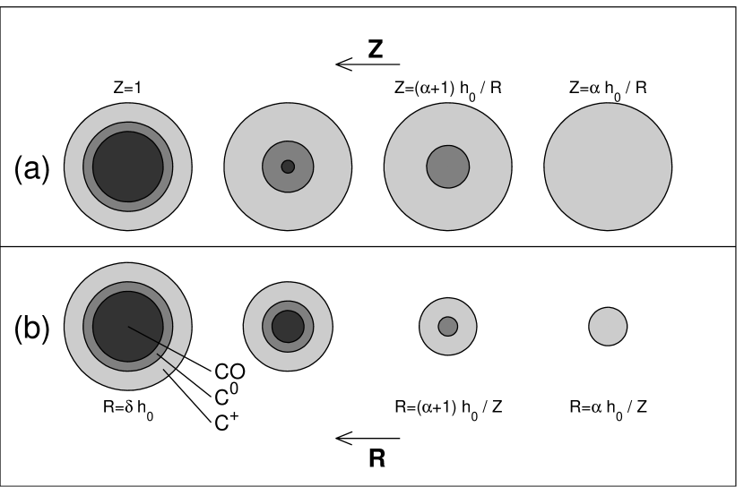
Figure 1: (a) Top Row. A sequence of clumps with identical radius and decreasing metallicity according to model A. When $Z={(\alpha+1)h_{0}/R}$, the CO is completely photodissociated and the clump consists only of C⁰ and C⁺. The next stage happens at $Z=\alpha h_{0}/R$, when all the neutral carbon is photoionized into C⁺. At even lower metallicities all the gas consists only of C⁺. (b) Bottom Row. A sequence of clumps with constant metallicity and decreasing radii in model A. Similar sequences where the limiting cases occur at slightly different metallicities can be created using model B.

All the material that is not photoionized (C⁺) or photodissociated (C⁰) is in molecular form (CO), and given the radius $R$ of a clump it is easy to compute the size of the CO region as $h_{\rm CO}=R-h-h_{+}$. Figure 1a illustrates how these scaling laws apply to a sequence of clumps with constant radius and decreasing metallicity. Conversely, Figure 1b illustrates the scaling laws applied to a sequence of clumps with constant metallicity and decreasing radius.

From the geometry and scaling laws the contribution of a clump of radius $R$ to the number of particles $\cal N$ of each species is

$$\cal N({\rm C}^{+}) = \left\{\begin{array}[]{lrcl}{4\over 3}\pi n\eta_{\rm C}(R^{3}-(R-\alpha h)^{3})&&R&>h_{+}\\ {4\over 3}\pi n\eta_{\rm C}R^{3}&0<&R&\leq h_{+}\end{array}\right.$$ (5)

$$\cal N({\rm C^{0}}) = \left\{\begin{array}[]{lrcl}{4\over 3}\pi n\eta_{\rm C}((R-\alpha h)^{3}-(R-(\alpha+1)h)^{3})&&R&>h+h_{+}\\ {4\over 3}\pi n\eta_{\rm C}(R-\alpha h)^{3}&h_{+}<&R&\leq h+h_{+}\\ 0&0<&R&\leq h_{+}\end{array}\right.$$ (9)

$$\cal N({\rm CO}) = \left\{\begin{array}[]{lrcl}{4\over 3}\pi n\eta_{\rm C}(R-(\alpha+1)h)^{3}&&R&>h+h_{+}\\ 0&0<&R&\leq h+h_{+}\end{array}\right.$$ (12)

where $\eta_{\rm C}$ is the carbon abundance and we are implicitly assuming that all the carbon is in the form of the dominant species in each zone. The abundance of carbon scales proportionally to $Z$, that is

$$\eta_{\rm C}=\eta_{0}Z$$ (13)

where $\eta_{0}$ is the carbon abundance at a metallicity $Z=1$.

We will now compute the mean contribution of a clump to the column density of each species, using CO as an example. To eliminate the dependence on clump size, we integrate Equation 12 over the clump size distribution $R^{-\beta}$ to obtain the mean contribution of a clump to the number of CO molecules in the telescope beam,

$$\overline{\cal N({\rm CO})}=\frac{1}{\cal M}\int_{R_{min}}^{R_{max}}{{\cal N(\rm CO)}R^{-\beta}\,dR}$$ (14)

where $R_{min}$ and $R_{max}$ are the lower and upper limits of the clump size distribution, and $\cal M$ is the normalization integral

$${\cal M}=\int_{R_{min}}^{R_{max}}R^{-\beta}\,dR$$ (15)

To simplify the calculations, we relate the lower and upper end of the clump size distribution to $h_{0}$ by defining $R_{min}\equiv\gamma h_{0}$ and $R_{max}\equiv\delta h_{0}$, where $\gamma$ and $\delta$ are unitless.

The total number of particles in the beam will be the number of clumps in it times the expected contribution per clump $\overline{\cal N({\rm CO})}$. Using $\beta=3$ and the fact that $\delta\gg\gamma$ we obtain an algebraic expression for ${\cal N({\rm CO})}$ which we convert to column density (and somewhat simplify) by recognizing that the expectation value for the radius of a clump is

$$\overline{R}=\frac{\int_{\gamma h_{0}}^{\delta h_{0}}R\ R^{-3}dR}{\int_{\gamma h_{0}}^{\delta h_{0}}R^{-3}dR}\cong 2\gamma h_{0}$$ (16)

Thus, dividing $\overline{\cal N({\rm CO})}$ by $\pi\overline{R}^{2}$ we obtain the mean CO column density per clump

$$\overline{N_{\rm CO}} = \left\{\begin{array}[]{lrcl}N_{0}\left[\frac{(\alpha+1)^{3}-6(\alpha+1)^{2}\delta Z+3(\alpha+1)\delta^{2}Z^{2}+2\delta^{3}Z^{3}}{2\delta^{2}Z^{2}}\right.\\ \left.\ \ \ \ \ \ \ \ \ \ \ +3(\alpha+1)\log\left(\frac{1+\alpha}{\delta Z}\right)\right]&&Z&>\frac{\alpha+1}{\delta}\\ 0&\frac{\alpha+1}{\delta}\geq&Z&>0\end{array}\right.$$ (20)

where we define $N_{0}\equiv{2\over 3}n_{\rm H}\eta_{0}h_{0}$. Notice that when $R_{max}\leq h+h_{+}$ even the biggest clump is completely photodissociated. As a result there is a critical metallicity $Z_{\rm CO}=(1+\alpha)/\delta$ below which CO is absent from the ensemble of clumps.

Proceeding similarly for Eqs. 5 and 9 we obtain the following expressions for the mean C⁺ and C⁰ column densities

$$\overline{N_{\rm C^{+}}} = \left\{\begin{array}[]{lrcl}N_{0}\left[\frac{-\alpha^{3}+6\alpha^{2}\delta Z-3\alpha\delta^{2}Z^{2}}{2\delta^{2}Z^{2}}+3\alpha\log\left(\frac{\delta Z}{\alpha}\right)\right]&&Z&>\frac{\alpha}{\delta}\\ N_{0}\ \delta Z&\frac{\alpha}{\delta}\geq&Z&>0\end{array}\right.$$ (23)

$$\overline{N_{\rm C^{0}}} = \left\{\begin{array}[]{lrcl}N_{0}\left[\frac{-(1+3\alpha+3\alpha^{2})+6(1+2\alpha)\delta Z-3\delta^{2}Z^{2}}{2\delta^{2}Z^{2}}\right.\\ \left.\ \ \ \ \ \ \ \ \ \ \ +3\alpha\log\left({\frac{\alpha}{\alpha+1}}\right)+3\log\left(\frac{\delta Z}{\alpha+1}\right)\right]&&Z&>\frac{\alpha+1}{\delta}\\ N_{0}\left[\frac{\alpha^{3}-6\alpha^{2}\delta Z+3\alpha\delta^{2}Z^{2}+2\delta^{3}Z^{3}}{2\delta^{2}Z^{2}}+3\alpha\log\left(\frac{\alpha}{\delta Z}\right)\right]&\frac{\alpha+1}{\delta}\geq&Z&>\frac{\alpha}{\delta}\\ 0&\frac{\alpha}{\delta}\geq&Z&>0\end{array}\right.$$ (28)

Equations 20, 23 and 28 constitute model A.

Note that in this parametrization $\alpha$, the ratio of the sizes of the C⁺ and C⁰ regions, is also approximately the ratio of the C⁺ to C⁰ columns times a geometrical correction factor of order unity. This stems from the construction of the model ($\alpha$ is the ratio between the extents of the C⁺ and C⁰ regions) as well as from the limit of Equations 23 and 28 when ${{\delta Z}\over\alpha}\gg 1$ and $\alpha\sim 1$ (c.f., §5). In this limit the ratio ${N_{\rm C^{+}}}/{N_{\rm C^{0}}}$ is approximately

$$\frac{N_{\rm C^{+}}}{N_{\rm C^{0}}}\approx\alpha\frac{3\log(\frac{\delta Z}{\alpha})-1.5}{3\log(\frac{\delta Z}{\alpha})-4.3}\sim\alpha$$ (29)

The value of $\delta$ determines mainly the CO column, since the biggest clumps are mostly CO. Consequently a decrease in $\delta$ will increase both the ${N_{\rm C^{+}}}/{N_{\rm CO}}$ and the ${N_{\rm C^{0}}}/{N_{\rm CO}}$ ratios. Thus the effects of both parameters are relatively well separated.

3.2 Model B

We will reconsider now the scaling law for the C⁰ region, expressed in Equation 1. If most of the C⁰ is not originated by photoprocesses but by other chemical reactions not strongly dependent on UV photons, the neutral carbon column density may not scale as $Z^{-1}$ (c.f., Equation 1) but as a slower function of $Z$. As the limiting case, we will assume that the size of the C⁰ region is constant with metallicity

$$h=h_{0}$$ (30)

The size of the C⁺ region nevertheless will continue to scale with $Z^{-1}$, as C⁺ is indeed produced mainly by photoionization. Therefore Equation 2 still holds. The parameter $\alpha$ is then akin to the ratio of C⁺ to C⁰ column densities at the relative metallicity $Z=1$. The corresponding equations for the mean column densities of C⁺, C⁰ and CO are

$$\overline{N_{\rm C^{+}}} = \left\{\begin{array}[]{lrcl}{N_{0}}\left[\frac{-\alpha^{3}+6\alpha^{2}\delta Z-3\alpha\delta^{2}Z^{2}}{2\delta^{2}Z^{2}}+3\alpha\log\left(\frac{\delta Z}{\alpha}\right)\right]&&Z&>\frac{\alpha}{\delta}\\ {N_{0}}\ \delta Z&\frac{\alpha}{\delta}\geq&Z&>0\end{array}\right.$$ (33)

$$\overline{N_{\rm C^{0}}} = \left\{\begin{array}[]{lrcl}{N_{0}}\left[-\frac{3\alpha^{2}+3\alpha(1-4\delta)Z+(1-6\delta+3\delta^{2})Z^{2}}{2\delta^{2}Z}\right.\\ \left.\ \ \ \ \ \ \ \ \ \ \ \ \ \ \ \ \ +3\alpha\log\left(\frac{\alpha}{\alpha+Z}\right)+3Z\log\left(\frac{\delta Z}{\alpha+Z}\right)\right]&&Z&>\frac{\alpha}{\delta-1}\\ {N_{0}}\left[\frac{\alpha^{3}-6\alpha^{2}\delta Z+3\alpha\delta^{2}Z^{2}+2\delta^{3}Z^{3}}{2\delta^{2}Z^{2}}+3\alpha\log\left(\frac{\alpha}{\delta Z}\right)\right]&\frac{\alpha}{\delta-1}\geq&Z&>\frac{\alpha}{\delta}\\ 0&\frac{\alpha}{\delta}\geq&Z&>0\end{array}\right.$$ (38)

$$\overline{N_{\rm CO}} = \left\{\begin{array}[]{lrcl}{N_{0}}\left[\frac{\alpha^{3}+3\alpha^{2}(1-2\delta)Z+3\alpha(1-4\delta+\delta^{2})Z^{2}+(1-6\delta+3\delta^{2}+2\delta^{3})Z^{3}}{2\delta^{2}Z^{2}}\right.\\ \left.\ \ \ \ \ \ \ \ \ \ \ +3(\alpha+Z)\log\left(\frac{\alpha+Z}{\delta Z}\right)\right]&&Z&>\frac{\alpha}{\delta-1}\\ 0&\frac{\alpha}{\delta-1}\geq&Z&>0\end{array}\right.$$ (42)

Equations 33, 38 and 42 constitute model B. We compare the relative merits of both models in §7. Notice that models A and B produce identical results at $Z=1$.

4 Computing integrated line ratios

We can now compute the line intensities using our calculated column densities. Notice that the column density ratios between species depend only on two non-dimensional parameters: $\alpha$ (the ratio of sizes between the C⁺ and C⁰ regions) and $\delta$ (the ratio between the sizes of the biggest clump and the C⁰ region). To simplify the calculations we will assume optically thin emission in local thermodynamic equilibrium (LTE) for C⁺ and C⁰. The line integrated intensity (erg s^-1 cm^-2 sr^-1) is then

$${\rm I}={1\over 4\pi}h\nu A_{ul}\frac{g_{u}e^{-{h\nu\over kT_{ex}}}}{Q(T_{ex})}\,N$$ (43)

where $h$ and $k$ are Planck’s and Boltzmann’s constants; $\nu$, A_ul and T_ex are respectively the transition frequency, Einstein A coefficient and excitation temperature; $g_{u}$ is the degeneracy of the upper level; $Q$ is the partition function, and $N$ is the total column density of the species considered. Typically C⁺ and C⁰ have opacities $\tau\leq 1$ (Zmuidzinas et al. 1988). The assumption of LTE will be valid as long as most of the emitting gas is at a density greater than the critical density of the transition ($\sim 2500$ cm^-3 for [C II], $\sim 500$ cm^-3 for the 609 $\mu$m transition of [C I]).

The assumption of optically thin emission from a population in LTE is, however, unrealistic for CO. For computing CO (J=$1\rightarrow 0$) intensities we will use the proportionality factor between hydrogen column density and CO line intensity observed at Galactic metallicity, $X_{\rm CO}=3\times 10^{20}$ cm^-2/(K km s^-1) (Scoville & Sanders 1987). The CO and hydrogen column densities at $Z=1$ are related via the CO abundance $\eta_{0}$, $N_{\rm CO}=N_{\rm H}\eta_{0}$. Thus, the integrated line intensity (in erg s^-1 cm^-2 sr^-1) can be related to the CO column density in the following way

$${\rm I_{CO}}={2k\over\lambda_{10}^{3}}{\overline{N_{\rm CO}}\over{X_{\rm CO}\eta_{0}}}$$ (44)

where $\lambda_{10}$ is the wavelength of the J=$1\rightarrow 0$ CO transition, and the factor $2k\over\lambda_{10}^{3}$ comes from the conversion between velocity-integrated antenna temperature and frequency-integrated specific intensity. In this expression we are implicitly assuming that the emissivity of CO, determined by the excitation conditions of the molecule, does not depend on $Z$. All the dependence of ${\rm I_{CO}}$ on the metallicity stems from the metallicity dependence of $\overline{N_{\rm CO}}$. This assumption will be discussed further in §8.

For the optically thin emission from [C II] (²P${}_{3/2}\rightarrow^{2}$P_1/2, 158 $\mu$m) and [C I] (³P${}_{1}\rightarrow^{3}$P₀, 609 $\mu$m) we assume excitation temperatures of 200 K and 30 K respectively (Wolfire, Hollenbach, & Tielens 1989; Wright et al. 1991). Thus,

$${\rm I_{[CII]}} = 1.28\times 10^{-21}\,\overline{N_{\rm C^{+}}}$$

$${\rm I_{[CI]}} = 7.54\times 10^{-24}\,\overline{N_{\rm C^{0}}}$$ (45)

$${\rm I_{CO}} = 1.73\times 10^{-26}\,\overline{N_{\rm CO}}$$

where we are using the canonical value $\eta_{0}=3\times 10^{-4}$ (e.g., Tielens & Hollenbach 1985a) and the line intensities are in units of erg s^-1 cm^-2 sr^-1. The equations for line ratios then are

$${\rm I_{[CII]}}/{\rm I_{CO}} = 7.4\times 10^{4}\,\overline{N_{\rm C^{+}}}/\overline{N_{\rm CO}}$$

$${\rm I_{[CI]}}/{\rm I_{CO}} = 4.4\times 10^{2}\,\overline{N_{\rm C^{0}}}/\overline{N_{\rm CO}}$$ (46)

$${\rm I_{[CII]}}/{\rm I_{[CI]}} = 1.7\times 10^{2}\,\overline{N_{\rm C^{+}}}/\overline{N_{\rm C^{0}}}$$

where only two of the three equations are independent.

Note that because [C II] and [C I] are a two and a three level system respectively, the intensities are independent of the precise value of the temperature as long as it exceeds the line excitation threshold.

5 The values of the parameters $\alpha$ and $\delta$

We can use Galactic data to assign values to $\alpha$ and $\delta$. In particular, we could use COBE’s FIRAS measurements averaged over the entire galactic plane. Unfortunately FIRAS did not obtain a significant detection of the CO (J=$1\rightarrow 0$) transition. This opens a range of possibilities for the CO intensity: 1) the formal value obtained by FIRAS ($0.6\pm 0.7$ erg s^-1 cm^-2 sr^-1; Wright et al. 1991), 2) the result of a multi-line excitation fit performed with the higher transitions of CO which FIRAS did detect (0.5 erg s^-1 cm^-2 sr^-1; Wright et al. 1991), or 3) the result of assuming the standard empirical ratio ${\rm I_{[CII]}/I_{CO}}=4400$ (Wolfire et al. 1989), which corresponds to a CO (J=$1\rightarrow 0$) intensity of 0.4 erg s^-1 cm^-2 sr^-1 given the observed FIRAS [C II] intensity of $1726\pm 70$ erg s^-1 cm^-2 sr^-1. Adopting the intermediate value ${\rm I_{CO}}=0.5$ erg s^-1 cm^-2 sr^-1 we obtain the ratios ${\rm I_{[CII]}/I_{[CI]}}\cong 270$ and ${\rm I_{[CI]}/I_{CO}}\cong 13$ from the FIRAS measurements. Numerically solving the system of Equations 46 we find the values $\alpha\cong 1.25$ and $\delta\cong 435$. Note that this result is independent of the choice of model A or B, since as was pointed out before both models are identical at $Z=1$.

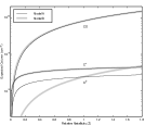
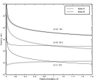
Figure 2: (a) Top. The mean column densities of CO, C⁰ and C⁺ versus metallicity resulting from models A and B. The values used for the hydrogen density and the size of the C⁰ region for the purpose of the plot are $n=10^{4}$ cm^-3 and $h_{0}=10^{17}$ cm ($\sim 0.03$ pc). (b) Bottom. The line intensity ratios versus metallicity for models A and B. Notice that, in model A, the [C II]/[C I] ratio is almost constant over a wide range of relative metallicities, while in model B the [C I] to CO ratio is approximately constant.

The resulting column density and line intensity ratios are shown in Figure 2. With the above values for $\alpha$ and $\delta$, the ratio of C⁺ to C⁰ column densities in model A yields $N_{\rm C^{+}}/N_{\rm C^{0}}\approx 1.65\pm 0.10$ over a wide range of metallicities. In model B the quantity that is approximately conserved for different metallicities is the ratio of C⁰ to CO column densities, and consequently the ratio of intensities.

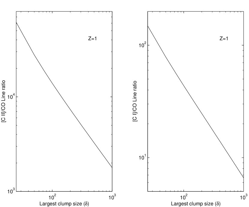
Figure 3: The influence of the upper limit of the clump size distribution (i.e., the parameter $\delta$) on the model ratios at Galactic metallicity ($Z=1$). The biggest clumps contribute mostly CO to the ensemble; consequently the line ratios decrease for higher clump sizes.

It is interesting to point out again that lowering the value of the maximum clump size $R_{max}$ (set by $\delta$) increases the column densities of C⁺ and C⁰. This occurs because the biggest clumps contribute mostly molecular (CO) gas. In fact, they dominate the CO column density. The effects on the line ratios of varying the maximum size parameter $\delta$ are shown in Figure 3. Some of the abnormally high [C II]/CO intensity ratios observed in certain sources could be due to a local change in the clump size distribution, caused by the disruption of the biggest clumps.

6 The effects of density and radiation fields

Up to this point, our parametrization has been purely geometrical. We have not explicitly included changes in the gas density ($n$) or the radiation field intensity ($\chi_{\rm uv}$). We can introduce these changes through their effects on the parameters $\alpha$, $\delta$ and $h_{0}$.

According to chemistry calculations (van Dishoeck & Black 1988), at a hydrogen density $n=10^{4}$ cm^-3 the C⁺ column density increases by a factor of $\sim 10$ when $\chi_{\rm uv}$ is increased from 1 to $10^{4}$ (in units of $1.6\times 10^{-3}$ erg cm^-2 s^-1; Habing 1968), while the C⁰ column density increases roughly a factor of $\sim 2$ to 3. Thus, the column density of C⁰ (controlled by the parameter $h_{0}$) as well as the ratio of the C⁺ to C⁰ column densities (controlled by the parameter $\alpha$) are both somewhat affected by the UV field strength, albeit not dramatically. The logarithmic dependence of the column densities on the radiation field occurs because, at densities larger than $\sim 10^{3}$ cm^-3, the column density of the species produced by photoprocesses varies proportionally to the penetration depth of the UV radiation, which in turn increases logarithmically with $\chi_{\rm uv}$ (Stacey et al. 1991; see also discussion in Mochizuki et al. 1996). On these grounds, we surmise that both $\alpha$ and $h_{0}$ are directly proportional to the logarithm of $\chi_{\rm uv}$. Assuming that the upper end of the clump size distribution, $R_{max}=\delta h_{0}$, remains unaffected by the UV field strength, $\delta$ is inversely proportional to $h_{0}$.

A qualitative argument can be used to understand how changes in the density will affect $h_{0}$, $\alpha$ and $\delta$. Higher densities will yield higher recombination rates for C⁺ and the more active chemistry will produce more CO at the expense of C⁰ and C⁺. Although it is a priori unclear how the column densities of C⁺ and C⁰ depend on the density, chemical modelling (Ingalls 1998) shows that it is also approximately logarithmic.

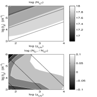
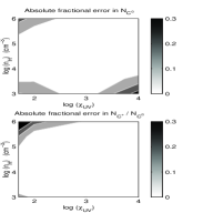
Figure 4: (a) Left Column. Two dimensional fits to the results of a chemical model (Ingalls 1998) for $\log N_{C^{0}}$ and $\log(N_{C^{+}}/N_{C^{0}})$. The gray scale corresponds to the results of the chemical network. The black contours are traced at the same levels and show the quality of the fits. (Top Left) Contour levels are 10¹⁷ to 10¹⁸ cm^-2 with logarithmic spacing 0.2. (Bottom Left) Contour levels are -0.05 to 0.1 with logarithmic spacing 0.05. (b) Right Column. Errors introduced by using the fits ($F$) rather than the actual results of the chemical network ($N$), expressed as $|N-F|/N$. The RMS error for $N_{C^{0}}$ and $N_{C^{+}}/N_{C^{0}}$ over the whole range of density and UV field shown here are 11% and 8% respectively. Contour levels are 10% to 30% by 10%.

Figure 4 shows the results of the steady-state chemical network calculations on an $A_{V}\geq 8$ cloud. Superimposed are the 2-dimensional fits to the chemistry results:

$$\log N_{C^{0}} \cong 0.13\log\chi_{\rm uv}-0.18\log n+18.32$$ (47)

$$\log\left(\frac{N_{C^{+}}}{N_{C^{0}}}\right) \cong 0.05\log\chi_{\rm uv}+0.02\log n-0.16$$ (48)

These equations are valid over a wide range of physical conditions ($\chi_{\rm uv}\sim 50-10^{4}$; $n\sim 10^{3}-10^{6}$ cm^-3) and the errors introduced by using the fits over the actual chemical network results are $\approx 10\%$.

The column densities of C⁺ and C⁰ obtained from Eqs. 47 and 48 can be directly related to the parameters $\alpha$ and $h_{0}$ by observing that, to first order, $N_{C^{0}}\simeq n\eta_{0}h_{0}$ and $N_{\rm C^{+}}/N_{\rm C^{0}}\simeq\alpha$. These two equations, combined with $\delta\propto{h_{0}}^{-1}$ lead to:

$$\alpha \approx 1.25\left({\chi_{\rm uv}\over{\chi_{\rm uv0}}}\right)^{+0.05}\left({n\over n_{0}}\right)^{+0.02}$$ (49)

$$\delta \approx 435\left({\chi_{\rm uv}\over{\chi_{\rm uv0}}}\right)^{-0.13}\left({n\over n_{0}}\right)^{+1.18}$$ (50)

where $\chi_{\rm uv0}$ and $n_{0}$ are the average radiation field and volume density of the regions that dominate the FIRAS line emission used to assign $\alpha=1.25$ and $\delta=435$. Note that because HII regions probably dominate the FIRAS emission (Wright et al. 1991; Bennett et al. 1994), $\chi_{\rm uv0}\gg 1$. Since the FIRAS ratios are similar to those observed in many Galactic star-forming regions (in particular Orion) we normalize all values of density and UV field to those derived for Orion, namely $n_{0}\sim 10^{4}$ cm^-3 and $\chi_{\rm uv0}\sim 250$ (Tielens & Hollenbach 1985b; Stacey et al. 1993).

7 Comparison with observations

The predictions of models A and B can be directly compared with observational data. To properly accomplish this comparison we need [C II] and [C I] observations on a sample of objects of the same class with different metallicities. Unfortunately very little [C I] data is available on extragalactic sources of differing metallicities (c.f., Wilson 1997; Table 2) and only a few of them have been observed in [C II].

The data we use for the comparison are listed in Table 1. The selected sources are a set of star-forming regions with different metallicities which have been observed in [C II] and [C I]. To them we have added N 27 in the Small Magellanic Cloud (SMC), a source that does not yet have [C I] observations but which we expect will be important to probe our models because it has the lowest metallicity in the sample.

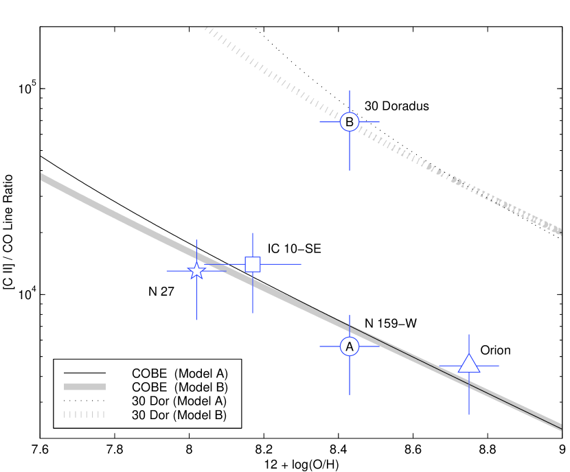
Figure 5: Comparison of model A and B predictions with [C II]/CO intensity ratios observed in several sources. The solid lines are the calculated [C II]/CO (J=$1\rightarrow 0$) intensity ratio with $\alpha$ and $\delta$ derived from the COBE FIRAS ratios. The dotted line corresponds to the COBE-based $\alpha$ and $\delta$ corrected in the way prescribed in §6 by assuming that for 30 Doradus $\chi_{\rm uv}=3500$ and $n=2000$ cm^-3. The data points are: the Orion interface region (triangle), N 159 in the LMC (circle A), 30 Doradus (circle B), IC 10 SE (square), and N 27 in the SMC (star). The error bars in the ratio are calculated assuming 30 % calibration accuracy in both lines.

Figure 5 compares the I_[CII]/I_CO intensity ratio predictions of models A and B with the observational data, using the values for $\alpha$ and $\delta$ derived from FIRAS measurements. Both models give essentially identical predictions for the decreasing trend in the I_[CII]/I_CO intensity ratio with increasing metallicity. This similarity between models A and B should not be surprising, since the effect of keeping $h$ constant in a clump (as model B does) is to enlarge its CO region by only a small fraction for $Z<1$, with respect to the same clump in model A. The fact that the I_[CII]/I_CO ratio for most sources (except 30 Doradus) falls along the model line can be interpreted as showing that N 27, IC 10-SE, N 159 and Orion all share similar values of $n$ and $\chi_{\rm uv}$. Another possibility is that the density and UV field in these regions conspire in such a way as to keep their line ratios close to the model line. This can happen because, as shown in Equation 50, the effects of density and radiation field go in opposite directions and have the potential to cancel each other. Denser regions, which are expected to have lower column densities of C⁺ and C⁰, will be in general more efficient at producing stars and thus will have on average a higher UV field which in turn will increase $N_{\rm C^{+}}$ and $N_{\rm C^{0}}$. However, because of the large difference in the exponents in Equation 50, this cancellation is unlikely to occur and we can safely assume that these star-forming regions posses similar densities and radiation fields.

The large ${\rm I_{[CII]}/I_{CO}}$ ratio observed in 30 Doradus suggests either that the gas in this source is under quite different physical conditions, or that $R_{max}$, the upper limit of the clump size distribution, is actually smaller than for the rest of the sample. Lowering the size of the biggest clump (by making $\delta$ smaller) will produce more photoionized material at the expense of CO, which will in turn raise the observed line ratio (c.f., §5). The gas in 30 Doradus is under an extremely intense (and hard) UV field, $\chi_{\rm uv}\simeq 3500$ (Poglitsch et al. 1995). From the numerical exponents of the relationships postulated in §6 (c.f., Equations 50 and 50), an increase by a factor of 15 in $\chi_{\rm uv}$ with respect to Orion (c.f., Table 1) is not enough to explain the observed line ratio. The average gas density must also decrease to about 2000 cm^-3, about 5 times lower than Orion’s. This density is within the range allowed by previous determinations (Poglitsch et al. 1995). Thus, it is not necessary to invoke a smaller maximum clump size to explain the observed [C II]/CO line ratio, although it remains a logical possibility (e.g., Pak et al. 1998). The 30 Doradus nebula is an especially active massive star-forming region, and as such it is the site of several violent events which could disrupt the larger molecular clumps.

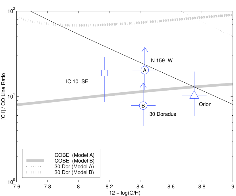
Figure 6: Same as figure 5 but for [C I]/CO intensity ratios versus metallicity. The point for IC 10-SE correspond to the average ratio in the complex (Bolatto et al. 1998). The point for 30 Doradus has been slightly displaced in metallicity to eliminate confusion in the error bars.

Figure 6 illustrates the comparison between the I_[CI]/I_CO intensity ratio predictions of models A and B and the observations. In this case the predictions of the two models differ drastically. While model A predicts a ratio that rapidly increases for decreasing metallicities, such a trend is not apparent in the observational data, which tends to cluster around a ratio of $\sim 10$, essentially the prediction of model B. Both Large Magellanic Cloud (LMC) points obtained by AST/RO (Stark et al. 1997) are lower limits to the ratio because of pointing uncertainties. They are roughly consistent with either model at the metallicity of the LMC, although N 159 favors model A while the discrepancy in the case of 30 Doradus is smaller with model B. A stronger constraint is provided by the IC 10-SE [C I] observations (Bolatto et al. 1998), which would have to be a factor of $\sim 2$ more intense in [C I] in order to be compatible with model A. An added complexity in the interpretation of the ratios in IC 10-SE is that the [C II] observations have a much larger beam size than the [C I] (approximately 60 arcsec and 10 arcsec respectively). Therefore, the I_[CII]/I_CO ratio may be sampling parcels of gas under much different physical conditions from those sampled by the I_[CI]/I_CO, a fact that could make the ratio observed in IC 10-SE appear artificially low.

Stronger constraints on the models would be provided by [C I] observations of the SMC. If this trend of constant ${\rm[C~{}I]/CO}$ intensity ratio is confirmed, we are led to conclude that most of the C⁰ in the clumps is not created by photodissociation but by other chemical processes. Otherwise, we would expect the trends of [C II]/CO and [C I]/CO intensity ratios with metallicity to be similar, as in model A.

8 The value of $X_{\rm CO}$

The proportionality between the CO emission intensity and the column density of H₂, $N_{\rm H_{2}}=X_{\rm CO}$I_CO, has been observationally established using different methods (see Magnani & Onello 1995 for a review of the methods and their caveats). The proportionality is well accepted for giant molecular clouds (GMCs), although the precise mechanisms by which $X_{\rm CO}$ becomes relatively independent of the physical conditions in the cloud remain unclear (e.g., McKee 1989).

There are a few observational determinations in the literature of the dependence of $X_{\rm CO}$ on metallicity $Z$. Using interferometric CO observations to obtain virial mass estimates of extragalactic GMC complexes, Wilson (1995) found a power law dependence with a slope of $-0.67$. Using a combination of single-dish and interferometric CO data and virial mass estimates, Arimoto et al. (1996) find a slope of $-0.8$.

In the context of the models presented here, we can use Equation 44 to investigate the expected dependence of $X_{\rm CO}$ on metallicity. Accordingly

$$\frac{X_{\rm CO}(Z)}{X_{\rm CO}(Z=1)}=\frac{\overline{N_{\rm CO}}(Z=1)}{\overline{N_{\rm CO}}(Z)}$$ (51)

and thus $X_{\rm CO}$ is inversely proportional to the mean column density of CO. The resulting slope with metallicity, according to Equations 20 or 42, is $\approx-1$.

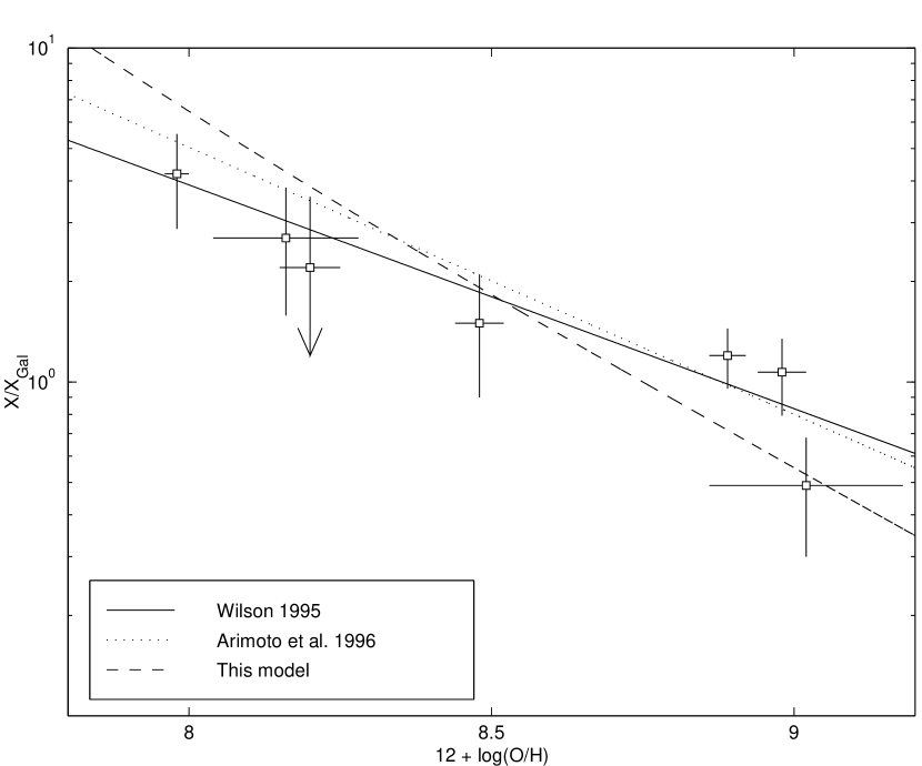
Figure 7: The CO (J=$1\rightarrow 0$) intensity to hydrogen column density conversion factor ($X_{CO}$) versus metallicity, as predicted by the models and deduced from observations. The data points are those used by Wilson (1995). The solid line corresponds to Wilson’s best fit with a slope of $-0.67$. The dotted line is a similar result obtained by Arimoto et al. (1996) using an independent data set. The slope of Arimoto’s best fit is $-0.8$. The dashed line represents the result of the models here developed, as explained elsewhere in the text. The slope is $-1.05$. Models A and B produce nearly identical results.

A comparison of our models with the results from Wilson (1995) and Arimoto et al. (1996) is shown in Fig. 7. The precise value of the clump size distribution exponent $\beta$ or the parameters $\alpha$ and $\delta$ do not affect the value of this slope, which mainly depends on the dominant term of the polynomial part of $\overline{N_{\rm CO}}$. Although the Wilson (1995) data points certainly fit a $-0.67$ slope better, the quality of the data does not exclude a slope closer to $-1$. A similar situation occurs with the Arimoto et al. (1996) data.

One of the reasons why the actual slope could be different from the theoretical expectation is a systematic change in the CO excitation temperature with metallicity. Such a dependence might be expected, since both the heating ($\Gamma$) and cooling ($\Lambda$) of the gas are affected by metallicity. The $\Gamma$ term is fundamentally controlled by photoelectric ejection of electrons from dust grains, which collisionally heat the gas. The cooling term is controlled by emission in the [C II], [O I] and [C I] fine structure transitions. The balance of the system at different metallicities and dust-to-gas ratios has been computed by Wolfire et al. (1995), who conclude that the temperature of the gas is higher for low $Z$. If the excitation temperature of CO is higher at low metallicities, the column of CO needed to produce a given intensity I_CO will drop, together with the corresponding column density of H₂. Consequently, there will be a drop in the $X_{\rm CO}$ factor as $X_{\rm CO}=N_{\rm H_{2}}/{\rm I_{\rm CO}}$ which will tend to flatten the curve of $X_{\rm CO}(Z)$.

9 Summary and conclusions

We have presented a model of PDRs of varying metallicity that depends on only two free parameters ($\alpha$, the ratio of sizes between the C⁺ and C⁰ regions and $\delta$, a measure of the size of the biggest clump in the ensemble). This approach naturally incorporates the clumpiness of the interstellar medium into the calculations and, when combined with some simple scaling laws, allows us to study the influence of metallicity on the PDR line emission. We have shown how to modify it to include the effects of density and radiation field, and we have used it to study the dependence of the ${\rm I_{[CII]}/I_{CO}}$ and ${\rm I_{[CI]}/I_{CO}}$ line ratios on the metallicity. In comparing our calculations with observational data, we find that the model explains well the observed trend of enhanced ${\rm[C~{}II]/CO}$ line ratio with decreasing metallicity as the natural result of the augmented fraction of photodissociated gas in a clump. We have shown that enhanced ratios can be produced by lowering the density or increasing the radiation field in the ISM, but also by lowering the upper limit of the clump size distribution as may happen in 30 Doradus (Pak et al. 1998). We find that the available data favors a ${\rm[C~{}I]/CO}$ intensity ratio essentially independent of metallicity, albeit the paucity of observations does not exclude other possibilities. This is difficult to understand if most of the C⁰ is produced by UV photons as is the case with C⁺, arguing for a chemical origin for at least part of the neutral carbon in these star-forming regions. More [C II] and [C I] observations on low metallicity sources such as the Small Magellanic Cloud are necessary, however, to establish this point. Finally, we have studied the prediction of the model for the trend of the $X_{\rm CO}$ factor with metallicity and compared it to previous observational studies, and we find that the agreement is reasonable.

Table 1: Source metallicities and intensity ratios

Source	12+log(O/H)	$\chi_{\rm uv}$	$n$	I[CII]/ICOa	I[CI]/ICOa	References
			(cm-3)
Milky Way	(8.75)$\ {}^{b}$			3450$\phantom{0}{}^{c}$	0.13$\ {}^{c}$	Wright et al. 1991, Bennet et al. 1994
Orion	8.75string	250	$10^{4}$string	4500	10 - 15	Lequeux et al. 1979, Stacey et al. 1993,
						Tauber et al. 1995
N 159 (LMC)	8.43string	300	$8\times 10^{3}\ {}^{d}$	5600	$\geq 20$	Dufour 1984, Israel et al. 1996,
						Stark et al. 1997
30 Doradus (LMC)	8.43string	3500	$10^{3}$ - $10^{4}$string	69000	$\geq 8$	Poglitsch et al. 1995, Stark et al. 1997
IC 10 SE (IC 10)	8.17string	$\ldots$	$\ldots$	14000	0.19$\ {}^{e}$	Lequeux et al. 1979,
						Madden et al. 1997, Bolatto et al. 1998
N 27 (SMC)	8.02string	$\ldots$	$\ldots$	13000	…	Dufour 1984, Israel et al. 1993
						Rubio et al. 1993

References

- (1) Abgrall, H., Le Bourlot, J., Pineau des Forêts, G., Roueff, E., Flower, D. R., & Heck, L. 1992, A&A, 253, 525
- (2)
- (3) Arimoto, N., Sōfue, Y., & Tsujimoto, T. 1996, PASJ, 48, 275
- (4)
- (5) Bennett, C. L. et al. 1994, ApJ, 434, 587
- (6)
- (7) Bolatto, A. D., Jackson, J. M., Wilson, C. D., & Moriarty-Schieven, G. 1998 in preparation
- (8)
- (9) Bouchet, P., Lequeux, J., Maurice, E., Prévot, L., & Prévot-Burnichon, M. L. 195, A&A, 149, 330
- (10)
- (11) Cohen R. S., Dame T. M., Garay G., Montani J., Rubio M., & Thaddeus P. 1988, ApJ, 331, L95
- (12)
- (13) Dufour, R. J. 1984, in Structure and Evolution of the Magellanic Clouds, ed. S. van der Bergh & K. S. de Boer (Dordrecht:Kluwer), 353
- (14)
- (15) Elmegreen, B. G. 1989, ApJ, 338, 178
- (16)
- (17) Elmegreen, B. G., & Falgarone, E. 1996, ApJ, 471, 816
- (18)
- (19) Habing, H. J. 1967, Bull. Astron. Inst. Netherlands, 19, 421
- (20)
- (21) Hollenbach, D. J., Takahashi, T., & Tielens, A. G. G. M. 1991, ApJ, 377, 192
- (22)
- (23) Ingalls, J. G., Bania, T. M., & Jackson, J. M. 1994, ApJ, 431, L139
- (24)
- (25) Ingalls, J. G., Chamberlin, R. A., Bania, T. M., Jackson, J. M., Lane, A. P., & Stark, A. A. 1997, ApJ, 479, 296
- (26)
- (27) Ingalls, J. G. 1998, Ph. D. Thesis
- (28)
- (29) Israel, F.P. 1988, in Millimetre and Submillimetre Astronomy, ed. R. D. Wolstencroft & W. B. Burton (Dordretch:Kluwer), 281
- (30)
- (31) Israel, F.P. et al. 1993, A&A, 276, 25
- (32)
- (33) Israel, F. P., Maloney, P. R., Geis, N., Hermann, F., Madden, S.C., Poglitsch, A., & Stacey, G. J. 1996, ApJ, 465, 738
- (34)
- (35) Johansson, L. E. B., Olofsson, H., Hjalmarson, Å., Gredel, R., & Black, J. H. 1994, A&A, 292, 371
- (36)
- (37) Keene, J., Young, K., Phillips, T. G., Buettgenbach, T. H., & Carlstrom, J. E. 1993, ApJ, 415, L131
- (38)
- (39) Koornneef, J. 1982, A&A, 107, 247
- (40)
- (41) Larson, R. B. 1981, MNRAS, 194, 809
- (42)
- (43) Le Bourlot, J., Pineau des Forêts, G., Roueff, E., & Flower, D. R. 1993, A&A, 267, 233
- (44)
- (45) Leisawitz, D. 1990, ApJ, 359, 319.
- (46)
- (47) Lequeux, J., Peimbert, M., Rayo, J. F., Serrano, A., & Torres-Peimbert, S. 1979, A&A, 80, 155
- (48)
- (49) Lequeux, J., Le Bourlot, J., Pineau des Forêts, G., Roueff, E., Boulanger, F., & Rubio, M. 1994, A&A, 292, 371
- (50)
- (51) Madden, S. C., Poglitsch, A., Geis, N., Stacey, G. J., & Townes, C. H. 1997, ApJ, 483, 200
- (52)
- (53) Maloney, P. 1990, in The Interstellar Medium in Galaxies, ed. H. A. Thronson, & J. M. Shull (Dordretch:Kluwer), 493
- (54)
- (55) Maloney, P., & Black, J. H. 1988, ApJ, 325, 389
- (56)
- (57) Magnani, L., & Onello, J. S. 1995, ApJ, 443, 169
- (58)
- (59) McKee, C. F. 1989, ApJ, 345, 782
- (60)
- (61) Mochizuki, K. et al. 1996, ApJ, 430, L37
- (62)
- (63) Myers, P. C. 1983, ApJ, 270, 105
- (64)
- (65) Pak, S., Jaffe, D. T., van Dishoeck, E. F., Johansson, L. E. B., & Booth, R. S. 1998, ApJ, 498, 735
- (66)
- (67) Plume, R., Jaffe, D. T., & Keene, J. 1994, ApJ, 425, L49
- (68)
- (69) Poglitsch, A., Krabbe, A., Madden, S. C., Nikola, T., Geis, N., Johansson, L. E. B., Stacey, G. J., & Sternberg, A. 1995, ApJ, 454, 293
- (70)
- (71) Rubio, M., Lequeux, J., & Boulanger, F. 1993, A&A, 271, 9
- (72)
- (73) Scoville, N. Z., & Sanders, D. B. 1987, in Interstellar Processes, ed. D. J. Hollenbach & H. A. Thronson (Dordrecht:Reidel), 21
- (74)
- (75) Savage, B. D., & Mathis, J. S. 1979, ARA&A, 17, 73
- (76)
- (77) Spaans, M. 1996, A&A, 307, 271
- (78)
- (79) Spaans, M., & van Dishoeck, E. F. 1997, A&A, 323, 953
- (80)
- (81) Spaans, M., & Neufeld, D. A. 1997, ApJ, 484, 785
- (82)
- (83) Stacey, G. J., Geis, N., Genzel, R., Lugten, J. B., Poglitsch, A., Sternberg, A., & Townes, C. H. 1991, ApJ, 373, 423
- (84)
- (85) Stacey, G. J., Jaffe, D. T., Geis, N., Genzel, R., Harris, A. I., Poglitsch, A., Stutzki, J., & Townes, C. H. 1993, ApJ, 404, 219
- (86)
- (87) Stark, A. A., Bolatto, A. D., Chamberlin, R. A., Lane, A. P., Bania, T. M., Jackson, J. M., & Lo, K.-Y. 1997, ApJ, 480, L59
- (88)
- (89) Sternberg, A., & Dalgarno, A. 1995, ApJS, 99, 565
- (90)
- (91) Stutzki, J., Stacey, G. J., Genzel, R., Harris, A. I., Jaffe, D. T., & Lugten, J. B. 1988, ApJ, 332, 379
- (92)
- (93) Stutzki, J., & Güsten, R. 1990, ApJ, 356, 513
- (94)
- (95) Tacconi, L. J., & Young, J. S. 1987, ApJ, 322, 681
- (96)
- (97) Tauber, J. A., Lis, D. C., Keene, J., Schilke, P., & Büttgenbach, T. H. 1995, A&A, 297, 567
- (98)
- (99) Tielens, A. G. G. M., & Hollenbach, D. 1985a, ApJ, 291, 722
- (100)
- (101) Tielens, A. G. G. M., & Hollenbach, D. 1985b, ApJ, 291, 747
- (102)
- (103) van Dishoeck, E. F., & Black, J. H. 1988, ApJ, 334, 771
- (104)
- (105) Wilson, C. D. 1995, ApJ, 448, L97
- (106)
- (107) Wilson, C. D. 1997, ApJ, 487, L49
- (108)
- (109) Wolfire, M. G., Hollenbach, D. J., & Tielens, A. G. G. M. 1989, ApJ, 344, 770
- (110)
- (111) Wolfire, M. G., Tielens, A. G. G. M., & Hollenbach, D. J. 1990, ApJ, 358, 116
- (112)
- (113) Wolfire, M. G., Hollenbach, D., McKee, C. F., Tielens, A. G. G. M., & Bakes, E. L. O. 1995, ApJ, 443, 152
- (114)
- (115) Wright, E. L. et al. 1991, ApJ, 381, 200
- (116)
- (117) Zmuidzinas, J., Betz, A. L., Boreiko, R. T., & Goldhaber, D. M. 1988, ApJ, 335, 774
- (118)