Microlensing towards the Small Magellanic Cloud
EROS 2 two-year analysis

Abstract

We present the analysis of the first two years of a search for microlensing of stars in the Small Magellanic Cloud with the eros (Expérience de Recherche d’Objets Sombres) project. A single event is detected, already present in the first year analysis. This low event rate allows us to put new constraints on the fraction of the Galactic Halo mass due to compact objects in the mass range [$10^{-2}$, $1$]$\>{\rm M}_{\odot}$. These limits, along with the fact that the two smc events observed so far are probably due to smc deflectors, suggest that lmc and smc self-lensing may dominate the event rate.

Galaxy: halo – Galaxy: kinematics and dynamics – Galaxy: stellar content – Magellanic Clouds – dark matter – gravitational lensing

1 Introduction

In 1986, B. Paczyński (Paczyński (1986)) proposed to use gravitational microlensing as a tool to probe the dark matter of the Galactic Halo. A few years later, several experiments started looking for microlensing events towards the Large Magellanic Cloud (lmc). Several candidates have now been observed by the macho and eros collaborations (Alcock et al. (1993); Aubourg et al. (1993), Alcock et al. 1997a, Ansari et al. (1996)).

The first results towards the lmc suggested an optical depth of order half that required to account for the dynamical mass of the dark halo, and the typical Einstein radius crossing time of the events implied a mass of about 0.5 M_⊙ for the lenses (Alcock et al. 1997a ). The results of the eros photographic plates microlensing survey pointed to a somewhat lower optical depth (Ansari et al. 1996). Such objects cannot be main-sequence stars, whose observed density is two orders of magnitude too low to account for the measured optical depth. Many hypotheses have been debated regarding the nature and location of these lenses, as LMC self-lensing (Sahu (1994); Wu (1994)), tidal debris (Zhao (1998)), intervening populations (Zaritsky & Lin 1997), a warped Galactic Disk (Evans et al. 1998), white dwarfs (Adams & Laughlin 1996, Graff et al. 1998), primordial black holes (Jedamzik 1998), all of which have brought forth numerous counter-arguments (Gould 1995, Alcock et al. 1997b, Gould 1998, Bennett 1998, Beaulieu & Sackett 1998). No fully satisfactory possibility has emerged, the main two trends being 0.5 M_⊙ dark objects in the halo, such as primordial black holes, or 0.1 M_⊙ main sequence stars near the lmc itself. The cosmological implications of these two hypotheses differ considerably.

The Small Magellanic Cloud (smc) is highly valuable as a second target for halo microlensing searches. If the lenses belong to the halo of our Galaxy, the optical depth and the distribution of event durations should be similar to the ones observed towards the lmc. In the case of smc or lmc self-lensing, however, the different dynamical properties of the two Clouds will give rise to differences in optical depth and event duration.

Eros, whose setup was upgraded in 1996, is engaged in observations towards the lmc and the smc. The analysis of the first year of observations towards the smc yielded one event (Palanque-Delabrouille et al. 1998, Alcock et al 1997c). A second event, whose source star was too faint to be in the eros reference catalog, was alerted on by macho and actively monitored by all microlensing collaborations. It was generated by a binary deflector most probably located in the smc itself (Afonso et al. (1998), Albrow et al. 1999, Alcock et al. 1999, Rhie et al. 1999, Udalski et al. 1999). This light curve, however, is not counted as an event in the following analysis which only uses stars identified on our template images, for which the efficiency can be estimated.

We present here the details of the eros 2 two-year analysis of data towards the smc  and discuss its implications for the nature of the halo dark matter.

2 Experimental setup and observations

The telescope, camera, telescope operations and data reduction are as described in Palanque-Delabrouille et al. 1998 and references therein. Ten square degrees are monitored on the smc. Note that since one ccd of the red camera was non functional, all the analysis is done on only 7 ccd’s (i.e. a total field of 8.6 square degrees).

The two-year data set contains 5.3 million light curves covering the period from July 1996 to March 1998.

3 Data analysis

The analysis of the two-year data set is similar to that of the first year (Palanque-Delabrouille et al. 1998). The major difference comes from the addition of rejection cuts requiring a minimum time coverage of the event (not possible with the previous one-year time span), and from the tuning of some cuts applied to parameters with a clear field-dependent distribution. The criteria are sufficiently loose not to reject light curves deformed by blending or by the finite size of the source, or events involving multiple lenses or sources. Most variable stars are rejected by at least two distinct cuts.

As in the first year analysis, we define a positive (negative) fluctuation as a series of data points that (i) starts by one point deviating by at least $1\sigma$ from the baseline flux $\phi_{0}$, (ii) stops with at least three consecutive points below $\phi_{0}+1\sigma$ (above $\phi_{0}-1\sigma$) and (iii) contains at least 4 points above $\phi_{0}+1\sigma$ (below $\phi_{0}-1\sigma$). The significance $LP$ of a given variation is defined as:

$$LP=-\sum_{i=1}^{i=N}\log\left(\frac{1}{2}\>{\rm Erfc}\left(\frac{x_{i}}{\sqrt{2}}\right)\right)$$ (1)

where $x_{i}$ is the deviation in $\sigma$’s of the point taken at time $t_{i}$ and $N$ the number of points within the fluctuation. We order the fluctuations along a light curve by decreasing significance. The cuts are described hereafter:
Selection of microlensing candidates:

• 1a: The main fluctuation detected in the red and blue light curves should be positive and occur simultaneously in the two colors: if I is the time interval during which the data are more than $1\sigma$ away from the baseline flux, we require $({\rm I_{red}}\cap{\rm I_{blue}})/({\rm I_{red}}\cup{\rm I_{blue}})>0.2$.

• 1b: To reject flat light curves with only statistical fluctuations, we require that on a given light curve
  $LP({\rm 2^{nd}\>most\>significant\>fluct.})\>/\>LP({\rm main\>fluct.})<0.6$
  in both colors.

• 1c: We require that $LP(\rm main\;fluct.)>30$ in both colors.

Rejection of variable stars:

• 2a: To exclude short period variable stars that exhibit irregular light curves, we require that the RMS of the distribution of the deviation, in $\sigma$’s, of each flux measurement from the linear interpolation between its two neighboring data points be small, typically less than 2.2 (the exact value varying from field to field, with a looser limit set on outer fields).

• 2b: To exclude variable stars which exhibit correlated fluctuations between the two colors, we calculate the correlation coefficient $\rho$ between the “red” and the “blue” light curves, excluding points in the main fluctuation (enlarged by a 25% time margin on either side) so as to consider only the un-amplified part of the light curve. The cut is applied to

  $${\rm cor}=\sqrt{N_{\rho}-2}\times{\rho}/{\sqrt{1-\rho^{2}}}$$

  whose distribution is less sensitive than $\rho$ to the number of points $N_{\rho}$. We require ${\rm cor}<6$.

• 2c: We remove two under-populated regions of the color-magnitude diagram that contain a large fraction of variable stars (upper main sequence and bright red giants, see details in first year analysis).

S/N improvement of the set of selected candidates:

• 3a: We remove events with low signal-to-noise ratio by requiring a significant improvement of a microlensing fit (ml) over a constant flux fit (cst), i.e. that
  $[\chi^{2}({\rm cst})-\chi^{2}({\rm ml})]/[\chi^{2}({\rm ml})/{\rm d.o.f.}]>\Delta\chi^{2}_{\rm min}$
  where d.o.f. is the number of degrees of freedom. As for cut 2a, the exact value of $\Delta\chi^{2}_{\rm min}$ varies from field to field because of the variations in time sampling. Typically, $\Delta\chi^{2}_{\rm min}\sim 350$, with a higher limit on well-sampled fields.

• 3b: We require that the maximum magnification in the microlensing fit be greater than 1.40.

Time coverage of the event:

• 4a: We require that the fitted time of maximum magnification be contained in the period of observation.

• 4b: We require that the fitted value of the Einstein radius crossing time $\Delta t<300$ days.

Physical blending:

• 5: If blending significantly improves the microlensing fit, then the fitted blending should be physical, i.e.: if $\chi^{2}({\rm no\;bl.})-\chi^{2}({\rm bl.})>10$, we require that the fitted blending fraction $f_{\rm bl}/f_{\rm tot}>-0.3$, in both colors.

The tuning of each cut and the estimation of the efficiency of the analysis (with the correction due to blending) is done with Monte Carlo simulated light curves, as described in Palanque-Delabrouille et al. 1998. The microlensing parameters are drawn uniformly in the following intervals: time of maximum magnification $t_{0}\in[t_{\rm first}-350,t_{\rm last}+350]$ days, impact parameter normalized to the Einstein radius $u_{0}\in[0,2]$ and time-scale $\Delta t\in[0,350]$ days. Cuts 2a and 3a are tuned individually on each field so as to reject respectively $\sim$ 15% and $\sim$ 25% of the remaining Monte Carlo light curves. The impact of each cut on data and simulated events is summarized in table 1.

	Number of	Fraction of remaining
Cut description	stars	stars removed by cut
	remaining	Data	Simulation
Stars analyzed	5,307,774	-	-
1a: Simultaneity	93,900	98%	76%
1b: Uniqueness	29,742	68%	11%
1c: Significance	9,978	66%	06%
2a: Stability	4,365	56%	16%
2b: Correlation	3,502	20%	02%
2c: HR diagram	2,996	14%	04%
3a: Microlensing fit	102	97%	24%
3b: Magnification	37	63%	16%
4a: Time inclusion	28	24%	20%
4b: Duration	22	21%	14%
5: Blending	1	95%	12%

Table 1: Impact of each cut on data and simulated microlensing events (allowing for blending). Each fraction for cut $n$ refers to the light curves remaining after cut $(n-1)$.

There is one remaining candidate, the one already discussed in the analysis of the first year data set. Its updated light curve is shown in figure 1.

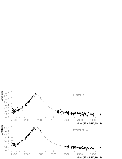
Figure 1: Light curve of microlensing event EROS-SMC-97/1 (the fit shown does not include the periodic modulation).

The efficiency of the analysis for events with an impact parameter $u_{0}<1$ and normalized to an observing period $T_{\rm obs}$ of one year is summarized in table 2, as a function of the Einstein radius crossing times $\Delta t$ (in days). The main source of systematics could come from a biased estimation of the blending effect. We have studied various blending models and found the relative error to be less than 10%.

$\Delta t$	7	22	37	52	67	100	150	250	300	350
$\epsilon$	4	12	16	18	21	24	25	23	13	3

Table 2: Efficiency (in %) of the analysis as a function of the time-scale $\Delta t$ (in days) for events with $u_{0}<1$, normalized to $T_{\rm obs}=1{\rm\>yr}$. We monitor $N_{\rm obs}=5.3\times 10^{6}$ stars.

4 Limits on the contribution of dark compact objects to the Halo

We fit a microlensing curve to the data of the candidate (see table 3), allowing for a periodic modulation of the source star as evidenced in the first year analysis. Blending and time-scale being degenerate quantities whose common fit is quite sensitive to systematics, we set the blending to that measured by ogle (Udalski et al. (1997)): $f_{\rm bl}/f_{\rm tot}\sim 24\%$, considering it to be a lower limit on the actual contribution (due to possible additional non-resolved companions). This value of the blending fraction is compatible with the absence of distorsion in the spectrum (Sahu (1998)).

$u_{0}$	$t_{0}$	$\Delta t$	$Period$	$A_{\rm mod\;R}$	$A_{\rm mod\;B}$
$0.424$	$2568.8$	$129$	$5.126$	$0.031$	$0.022$
$\pm 0.004$	$\pm 0.8$	$\pm 2$	$\pm 0.002$	$\pm 0.003$	$\pm 0.003$

Table 3: Result of microlensing fit to the smc event, with blending set to $f_{\rm bl}/f_{\rm tot}=25\%$. $t_{0}$ is the time of maximum magnification in days since Jan, 1 1990, $\Delta t$ the Einstein radius crossing time, in days. The $\chi^{2}$ is 261 for 279 d.o.f.

In order to set limits on the contribution of dark objects to the Halo, a Halo model must be used to obtain, for a given deflector mass, both a number of expected events and a distribution of event durations. We use the so-called “standard” halo model described in Palanque-Delabrouille et al. 1998 as model 1, and take into account the efficiency of the analysis given in the previous section.

Moreover, to set conservative limits, we have assumed that the observed event is a halo event, in spite of the fact that it is most probably an smc self-lensing event (Palanque-Delabrouille et al. 1998).

Assuming a standard halo model with a mass fraction $f$ composed of dark compact objects having a single mass $M$, the likelihood of observing at most one event, with a duration less probable than the observed one ($\Delta t_{\rm obs}$), is

$$L(M)=e^{-f\tilde{N}_{M}}\left(1+f\tilde{N}_{M}{\cal P}_{M}(\Delta t_{\rm obs})\right)$$ (2)

with

$${\cal P}_{M}(\Delta t_{\rm obs})=\int_{0}^{\Delta t_{1}}P_{M}(\Delta t)d\Delta t+\int_{\Delta t_{2}}^{\infty}P_{M}(\Delta t)d\Delta t$$ (3)

$\Delta t_{1}$ and $\Delta t_{2}$ are the two durations with the same probability as $\Delta t_{\rm obs}$, defined by:

$$P_{M}(\Delta t_{1})=P_{M}(\Delta t_{2}),\>\Delta t_{1}<\Delta t_{2},\>$$

$$(\Delta t_{1}=\Delta t_{\rm obs}\;\mathrm{or}\;\Delta t_{2}=\Delta t_{\rm obs})$$ (4)

$P_{M}(\Delta t)$ is the distribution of expected event durations, taking efficiencies into account, and $\tilde{N}_{M}$ is the expected number of events.

Figure 2 shows the 95 % exclusion limit derived from this likelihood function on $f$, the halo mass fraction, at any given mass $M$, i.e. assuming all deflectors in the halo have mass $M$. For comparison, the exclusion curve obtained considering that the sole event detected does not belong to the halo (thin dashed line on the plot) is also shown. The limit is very similar to the one event one, since the very long duration of the event pushes it towards large masses, where our efficiency starts to drop.

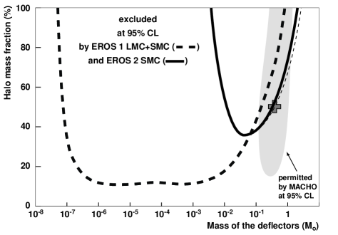
Figure 2: Exclusion diagram at 95 % C.L. for the standard halo model ($4\times 10^{11}\>{\rm M}_{\odot}$ inside 50 kpc). The dashed line is the limit from eros 1 lmc and smc data (Renault et al., 1997), the solid line is the limit from the smc data described in this paper. The macho 95 % C.L. accepted region is the shaded area, with the preferred value indicated by the cross (Alcock et al. 1997a). The thin dashed line corresponds to the limit obtained assuming we observed no halo events.

5 Discussion and conclusion

The analysis of two years of eros 2 smc data has yielded a single microlensing event. This allows us to put new constraints on the fraction of the halo made of objects in the range [$10^{-2}\>{\rm M}_{\odot}$, $1\>{\rm M}_{\odot}$], excluding in particular at the 95 % C.L. that more than 50 % of the standard halo be made of $0.5\>{\rm M}_{\odot}$ objects.

One should also note that all the microlensing events towards the lmc and the smc for which information could be obtained on the deflector location — through parallax for this 97-SMC-1 event (Palanque-Delabrouille et al. 1998), and deflector binarity for 98-SMC-1 and LMC-9 (but see the discussion in Bennett et al. 1996) — seem to be produced by deflectors located in the Clouds themselves. This suggests that self-lensing may be the dominant source of the observed events. We are continuing to accumulate data towards the lmc and smc in order to determine definitively the location of the deflectors.