International Journal of Modern Physics D,
©World Scientific Publishing Company

1

COSMIC STRINGS, LOOPS, AND

LINEAR GROWTH OF MATTER PERTURBATIONS

Jiun-Huei Proty Wu

Astronomy Department, University of California, Berkeley, 601 Campbell Hall,

Berkeley, CA 94720-3411, USA

Pedro P. Avelino

Centro de Astrofísica, Universidade do Porto, Rua das Estrelas s/n,

4150-762, Porto, Portugal

Dep. de Física da Faculdade de Ciências da Univ. do Porto, Rua do Campo Alegre 687,

4169-007, Porto, Portugal

E. P. S. Shellard

Department of Applied Mathematics and Theoretical Physics, University of Cambridge, Silver Street,

Cambridge CB3 9EW, UK

Bruce Allen

Department of Physics, University of Wisconsin–Milwaukee P.O. Box 413, Milwaukee,

Wisconsin 53201, U.S.A.

Received (received date)
Revised (revised date)

We describe a detailed study of string-seeded structure formation using high resolution numerical simulations in open universes and those with a non-zero cosmological constant. We provide a semi-analytical model which can reproduce these simulation results including the effect from small loops chopped of by the string network. A detailed study of cosmic string network properties regarding structure formation is also given, including the correlation time, the topological analysis of the source spectrum, the correlation between long strings and loops, and the evolution of long-string and loop energy densities. For models with $\Gamma\,=\,\Omega h\,=\,0.1$–$0.2$ and a cold dark matter background, we show that the linear density fluctuation power spectrum induced by cosmic strings has both an amplitude at $8h^{-1}$Mpc, $\sigma_{8}$, and an overall shape which are consistent within uncertainties with those currently inferred from galaxy surveys. The cosmic string scenario with hot dark matter requires a strongly scale-dependent bias in order to agree with observations.

1 Introduction

One of the outstanding problems in cosmology today is developing a more precise understanding of structure formation in the universe, that is, the origin of galaxies and other large scale structures. Existing theories for the structure formation of the Universe fall into two categories, based either upon the amplification of quantum fluctuations in a scalar field during inflation, or upon a symmetry breaking phase transition in the early Universe which leads to the formation of topological defects. While techniques for computing density perturbations for the former are well established,^?,?,? only little quantitative work exists for the latter due to calculational difficulties in modeling nonlinear effects, especially for cosmic string models.^?

The cosmic string scenario predated inflation as a realistic structure formation model,^? but it has proved computationally much more challenging to make robust predictions with which to confront observations. Only until recently, significant progress in understanding cosmic strings as seeds for large-scale structure and Cosmic Microwave Background Radiation (CMBR) anisotropies has been achieved.^{?,?,?,?,?,?,?,?,?} In this paper, we concentrate on local cosmic strings and describe a self-consistent method based on a fluid approximation to study string-seeded structure formation with either a cold or hot dark matter (CDM or HDM) background. The primary quantities of interest for comparing theories to observations are the power spectra of fluctuations, both for the mass density and the CMBR. In the work presented here, we concentrate only on the former but we will briefly discuss the latter. The present work relies on high-resolution numerical simulations of a cosmic string network,^? with a dynamic range extending from well before the matter-radiation transition through to deep into the matter era. Several important properties of local cosmic strings are revealed. The resulting power spectrum of linear density perturbations, ${\cal P}(k)$, and the mass fluctuation amplitude at $8h^{-1}$Mpc, $\sigma_{8}$, are calculated. A semi-analytic model is also introduced. It can reproduce the ${\cal P}(k)$ of our high-resolution simulations. We further investigate the dependence of ${\cal P}(k)$ on the curvature $K$ and the cosmological constant $\Lambda$. In particular, for models with $\Gamma\,=\,\Omega h\,=\,0.1$–$0.2$ and a CDM background, we show that both $\sigma_{8}$ and the overall shape of ${\cal P}(k)$ are consistent within uncertainties with those currently inferred from galaxy surveys. The HDM scenario with cosmic strings seems to require a large scale-dependent biasing in order to be consistent with observations.

The framework developed here is also suitable for investigating any other matter sources behaving stiffly, whose evolution is largely independent of the background matter and any inhomogeneities in the universe. This direct numerical approach marks a considerable quantitative advance by incorporating important aspects of the relevant physics not included in previous treatments. As such, the cosmic string power spectra presented here should be the most reliable to date.

The structure of the paper is as follows: In section 2, we investigate the linear perturbation equations for cosmic defect models in a flat $\Lambda$-universe. We then argue that this can be extended to closed and open universes for cosmic defect models. Section 3 starts by investigating the topology of generic sources. Then several important string properties are described, including the slow relaxation of the long-string and loop energy densities from the radiation to the matter era, the topology of string network, the string network correlation time, and the correlation between long strings and loops, etc. In section 4, we describe the approximation schemes invoked in this work, including the compensation of the source into the background, the inclusion of HDM, a semi-analytical model which can accurately reproduce the simulation results, and a simple extrapolation scheme which can generalize the simulation results from a flat $\Lambda=0$ model to open and flat $\Lambda$-models with any desired Hubble parameter. This simple scheme is then numerically verified with high accuracy. The unimportance of the late-time non-scaling behavior of strings in open or $\Lambda$-models is addressed. In section 5, we present the main results. Empirical formulae describing our main results are presented here. A brief discussion regarding the CMBR anisotropies is also given. Finally, a conclusion is given in section 6. We have defined the conventions of the background cosmology and given the analytical solutions for open, flat, close and $\Lambda$-models in Appendix A. Appendix 1 defines the conventions of our power spectrum and variance calculations. Through out the paper, we will use $h=0.7$, where the Hubble parameter is defined in the usual way $H=100h{\rm kms^{-1}Mpc^{-1}}$. A generalization of results from this choice to any other $h$ is provided in section 4.4.

2 Perturbation Equations

We consider density perturbations about a flat FRW model which are causally sourced by an evolving external-source network with energy-momentum tensor $\Theta_{\alpha\beta}({\bf x},\eta)$. In the synchronous gauge with a cosmological constant, the linear evolution of the radiation and CDM perturbations, $\delta_{\rm r}$ and $\delta_{\rm c}$ respectively, are given by (modified from Ref.^?)

$$\ddot{\delta}_{\rm c}+{\dot{a}\over a}\dot{\delta}_{\rm c}-{3\over 2}\Big{(}{\dot{a}\over a}\Big{)}^{2}\,\left(\Omega_{\rm c}\delta_{\rm c}+2\Omega_{\rm r}\delta_{\rm r}\right)=4\pi G\Theta_{+},$$ (1)

$$\ddot{\delta}_{\rm r}-{1\over 3}\nabla^{2}\delta_{\rm r}-{4\over 3}\ddot{\delta}_{\rm c}=0,~{}~{}~{}~{}~{}~{}~{}~{}~{}~{}$$ (2)

where $a(\eta)$ is the scale factor, $\Theta_{+}=\Theta_{00}+\Theta_{ii}$, a dot represents a derivative with respect to the conformal time $\eta$, and

$$\Omega_{\rm c}={a\over 1+a+Ba^{2}+Ca^{4}},\quad\Omega_{\rm r}={1\over 1+a+Ba^{2}+Ca^{4}},$$ (3)

with $B$ and $C$ defined in (A.3). Eqns. (1) and (2) are exact when $K=0$, i.e. $\Omega_{K0}=0$. However, they are still a very good approximation even if $K\neq 0$ because most perturbations on scales of interest are generated when the curvature-associated perturbation terms are small.

It proves useful to split these linear perturbations into initial (I) and subsequent (S) parts,^?

$$\delta_{N}({\bf x},\eta)=\delta_{N}^{\rm I}({\bf x},\eta)+\delta_{N}^{\rm S}({\bf x},\eta)\,,\qquad N={\rm c,r}\,,$$ (4)

with initial conditions

$$\delta_{N}^{\rm I}(\eta_{\rm i})=\delta_{N}(\eta_{\rm i}),\quad\dot{\delta}_{N}^{\rm I}(\eta_{\rm i})=\dot{\delta}_{N}(\eta_{\rm i}),$$ (5)

$$\delta_{N}^{\rm S}(\hat{\eta})=\dot{\delta}_{N}^{\rm S}(\hat{\eta})=0,\quad{\rm with}\,\eta>\hat{\eta}>\eta_{\rm i}\,.$$ (6)

In the case of topological defects, the initial perturbations $\delta^{\rm I}({\bf x},\eta)$ depend on the defect configuration at the defect formation time $\eta_{\rm i}$, because ultimately the formation of defects creates under-densities in the initially homogeneous background out of which they are carved. The subsequent perturbations $\delta^{\rm S}({\bf x},\eta)$ are those actively generated by the defects themselves for $\hat{\eta}>\eta_{\rm i}$. Because defects induce iso-curvature perturbations, $\delta^{\rm I}({\bf x},\eta)$ must compensate $\delta^{\rm S}({\bf x},\eta)$ on comoving scales $|{\bf x}-{\bf x}^{\prime}|>\eta$ to prevent acausal fluctuation growth on super-horizon scales, as we shall discuss later.

The system of eqns. (1) and (2) can be solved for the subsequent perturbations $\delta^{\rm S}({\bf x},\eta)$ by using a discretized version of the integral equation with Green functions:

$$\delta^{\rm S}_{N}({\bf x},\eta)=4\pi G\int_{\eta_{\rm i}}^{\eta}\!\!d\hat{\eta}\int d^{3}x^{\prime}\>{\cal G}_{N}(X;\eta,\hat{\eta})\Theta_{+}({\bf x^{\prime}},\hat{\eta}),\qquad N={\rm c,r}\,,$$ (7)

where $X=|{\bf x}-{\bf x^{\prime}}|$. The easiest method of obtaining the Green function solutions is to go to Fourier space and solve the resulting homogeneous system of ordinary differential equations numerically with appropriate initial conditions. Since the Green functions depend only on the modulus of $X=|{\bf x}-{\bf x^{\prime}}|$, it follows that their Fourier amplitudes must only depend on the modulus of ${\bf k}$. We will use a tilde $\;\widetilde{}\;$ to denote the Fourier transform of a function. With the change of variable $y=1+(\sqrt{2}-1)\eta/\eta_{\rm eq}$ and using (7), in Fourier space eqns. (1) and (2) with $K=\Lambda=0$ become

$$(1-y^{2}){\widetilde{\cal G}}_{\rm c}^{\prime\prime}-2y{\widetilde{\cal G}}_{\rm c}^{\prime}+\left[6-\frac{12{\widetilde{\cal G}}_{\rm r}/{\widetilde{\cal G}}_{\rm c}}{1-y^{2}}\right]{\widetilde{\cal G}}_{\rm c}=0\ ,$$ (8)

$$\widetilde{\cal G}_{\rm r}^{\prime\prime}-{4\over 3}\widetilde{\cal G}_{\rm c}^{\prime\prime}+{4k^{2}\over 3A^{2}}\widetilde{\cal G}_{\rm r}=0\ ,$$ (9)

with $A$ defined by (A.3), and initial conditions at $\eta=\hat{\eta}$ (or $\hat{y}=y(\hat{\eta})$) satisfying

$$\widetilde{\cal G}_{\rm r}=\widetilde{\cal G}_{\rm c}=0,\ \widetilde{\cal G}^{\prime}_{\rm r}=\frac{4}{3}\widetilde{\cal G}^{\prime}_{\rm c}=\frac{8}{3A}\,.$$ (10)

Here, a prime represents a derivative with respect to $y$ (though only in these equations).

Under certain limits, (8) and (9) can be solved analytically. When $k\eta\gg 1$, the radiation component will oscillate many times per expansion time and will have little net effect on the matter. So we can set $\widetilde{\cal G}_{\rm r}=0$ in this case and thus (8) decays to a homogeneous associated Legendre equation, whose solution is the linear combination of the two associated Legendre polynomials $P_{2}$ and $Q_{2}$. When $k\eta\ll 1$, by (9) and (10) we know $\widetilde{\cal G}_{\rm r}/\widetilde{\cal G}_{\rm c}=4/3$. So (8) decays to a homogeneous associated Legendre equation, whose solution is the linear combination of the two associated Legendre polynomials $P_{2}^{-4}$ and $Q_{2}^{4}$. One can therefore solve (8) and (9) with (10) for $\widetilde{\cal G}_{\rm c}$ under these limits to get:

$$\widetilde{\cal G}_{\rm c}(k;\eta,\hat{\eta})=\left\{\begin{array}[]{ll}\frac{2}{A}(\hat{y}^{2}-1)[{\cal A}(\hat{y}){\cal B}(y)-{\cal B}(\hat{y}){\cal A}(y)]\,,&k\eta\gg 1\,,\\ \frac{2}{A}(y^{2}-1)^{-1}[{\cal C}(\hat{y}){\cal D}(y)-{\cal D}(\hat{y}){\cal C}(y)]\,,&k\eta\ll 1\,,\end{array}\right.$$ (11)

where

$${\cal A}(y) = \left(\frac{3y^{2}-1}{4}\right)\log{\left(\frac{y+1}{y-1}\right)}-\frac{3y}{2}\,,$$ (12)

$${\cal B}(y) = \frac{3y^{2}-1}{2}\,,$$ (13)

$${\cal C}(y) = \frac{y}{y^{2}-1}\,,$$ (14)

$${\cal D}(y) = \frac{(y-1)^{3}(y^{2}+4y+5)}{5(y+1)}\,.$$ (15)

We notice that the scale factor $a(\eta)=y^{2}-1$. Because we are only interested in the matter perturbations at late times (i.e. today $\eta_{0}$) and we know from (8) that $\widetilde{\cal G}_{\rm c}\propto a/a_{\rm eq}=a$ when $\eta/\eta_{\rm eq}\rightarrow\infty$, what we actually need is the function:

$$\widetilde{T}_{\rm c}(k;\hat{\eta})\equiv\lim_{\eta/\eta_{\rm eq}\rightarrow\infty}\frac{1}{a}\widetilde{\cal G}_{\rm c}(k;\eta,\hat{\eta})\,.$$ (16)

Hence for $k\eta\rightarrow 0\;{\rm and}\;\infty$, we obtain from (11) that

$$\widetilde{T}_{\infty}(y(\hat{\eta})) = \frac{3}{A}(\hat{y}^{2}-1){\cal A}(\hat{y})\,,\quad k\eta\gg 1\,,$$ (17)

$$\widetilde{T}_{0}(y(\hat{\eta})) = \frac{2}{5A}{\cal C}(\hat{y})\,,\quad k\eta\ll 1\,.$$ (18)

Fig. 2 shows how (17) and (18) evolve with time.

Fig. 1. The evolution of the functions $T_{\rm c}(\eta)\equiv\widetilde{T}_{\rm c}(k;\hat{\eta})$ under the two limits: $k\eta\ll 1$ (dashed line), and $k\eta\gg 1$ (solid line).

Fig. 1. The evolution of the functions $T_{\rm c}(\eta)\equiv\widetilde{T}_{\rm c}(k;\hat{\eta})$ under the two limits: $k\eta\ll 1$ (dashed line), and $k\eta\gg 1$ (solid line).

Fig. 2 shows the numerical solutions of $\widetilde{\cal G}_{\rm c}(k;\eta_{0},\hat{\eta})$.

Fig. 2. The numerical solutions of $\widetilde{\cal G}_{\rm c}(k;\eta_{0},\hat{\eta})$. In the plot, $\eta\equiv\hat{\eta}$, and $G_{\rm c}\equiv\widetilde{\cal G}_{\rm c}(k;\eta_{0},\hat{\eta})$. The numbers attached to each lines indicate $\hat{\eta}/\eta_{\rm eq}$.

Fig. 2. The numerical solutions of $\widetilde{\cal G}_{\rm c}(k;\eta_{0},\hat{\eta})$. In the plot, $\eta\equiv\hat{\eta}$, and $G_{\rm c}\equiv\widetilde{\cal G}_{\rm c}(k;\eta_{0},\hat{\eta})$. The numbers attached to each lines indicate $\hat{\eta}/\eta_{\rm eq}$.

It confirms the asymptotic behaviors in these two regimes: on super-horizon scales ($k\ll 2\pi/\eta$), $\widetilde{\cal G}_{\rm c}(k;\eta_{0},\hat{\eta})$ scales as $\hat{\eta}^{-1}$, which is indicated by (18); on sub-horizon scales ($k\gg 2\pi/\eta$), the growth of matter perturbations has a maximum at $\hat{\eta}\sim\eta_{\rm eq}$, as seen in (17) (see also Fig. 2). We note that on sub-horizon scales, when going from $\hat{\eta}=0.05\eta_{\rm eq}$ to $\hat{\eta}=5\eta_{\rm eq}$, $\widetilde{\cal G}_{\rm c}(k;\eta_{0},\hat{\eta})$ changes only within a factor of $2$. Adding the fact that cosmic defects seed matter perturbations only on sub-horizon modes because on super-horizon scales they are compensated by the background and therefore can not create density perturbations, we see from Fig. 2 and 2 that defects induce power into matter perturbations mainly during the radiation-matter transition regime. This is generically different from inflationary models, in which matter perturbations are seeded during inflation in the deep radiation regime when all the modes are well outside the horizon.

Now we can obtain an approximated solution for the Green function by combining these two modes:

$$\begin{array}[]{lll}\widetilde{\cal G}_{\rm c}(k;\eta_{0},\hat{\eta})&\approx a_{\scriptscriptstyle 0}\widetilde{T}_{\rm c}(k;\hat{\eta})\vspace*{2mm}\\ &\approx a_{\scriptscriptstyle 0}\left\{\widetilde{T}_{\infty}+(\widetilde{T}_{0}-\widetilde{T}_{\infty})\left[1+(\alpha k\eta_{\rm eq})^{4/3}\right]^{-1}\right\}\vspace*{2mm}\\ &{\rm with}\ \left\{\begin{array}[]{ll}\alpha=0.75,&{\rm for\ 0.03<\hat{\eta}/\eta_{\rm eq}<125\ and\ 3{\it h}Mpc^{-1}<k},\\ \alpha=0.5,&{\rm for\ 0.2<\hat{\eta}/\eta_{\rm eq}}<125.\end{array}\right.\end{array}$$ (19)

The combination factor in (19) is a numerically verified guess and its accuracy is plotted in Fig. 2.

Fig. 3. The accuracy of eq. (19). $T_{\rm c}$ is equivalent to $\widetilde{T}_{\rm c}(k;\hat{\eta})$ in (19), while $G_{\rm c}\equiv\widetilde{\cal G}_{\rm c}(k;\eta_{0},\hat{\eta})$ is numerically calculated from (1) and (2) with initial conditions (10). In the legends, $\eta_{\rm i}\equiv\hat{\eta}/\eta_{\rm eq}$.

Fig. 3. The accuracy of eq. (19). $T_{\rm c}$ is equivalent to $\widetilde{T}_{\rm c}(k;\hat{\eta})$ in (19), while $G_{\rm c}\equiv\widetilde{\cal G}_{\rm c}(k;\eta_{0},\hat{\eta})$ is numerically calculated from (1) and (2) with initial conditions (10). In the legends, $\eta_{\rm i}\equiv\hat{\eta}/\eta_{\rm eq}$.

We note that the late-time positive departure of the accuracy (e.g. $\hat{\eta}=100,\,125\eta_{\rm eq}$, see Fig. 2) is caused by neglecting the negative terms associated with ${\cal B}(\hat{y})$ and ${\cal D}(\hat{y})$ in (11) when taking the limit (16) to get (17) and (18).

Finally, we obtain the subsequent perturbations in Fourier space today by integrating the Green function with the external source throughout the dynamical range within which the external source is present:

$$\widetilde{\delta}_{\rm c}^{\rm S}({\bf k},\eta_{0})=4\pi G\int_{\eta_{\rm i}}^{\eta_{0}}\widetilde{\cal G}_{\rm c}(k;\eta_{0},\hat{\eta})\widetilde{\Theta}_{+}({\bf k},\hat{\eta})d\hat{\eta}.$$ (20)

Here the Green function $\widetilde{\cal G}_{\rm c}(k;\eta_{0},\hat{\eta})$ can be either (19), or numerically obtained from eqns. (8) and (9) with initial conditions (10).

We also tested the performance of the fluid approximation (1) and (2), by computing the “transfer function” for primordial density perturbations in the absence of a source ($T_{k}$), defined as the ratio of the growing mode coefficient deep in the matter era to that deep in the radiation era. In Fig. 2, we compare our result with other previous work for the case of a flat universe with no cosmological constant. We see that although we have used the fluid approximation to model only the matter and radiation components, our result is only slightly larger with a maximum deviation being $5\%$ from the fit given by Bond and Efstathiou (BE),^? and $8\%$ from the result from CMBFAST,^? on the scale $k\sim 0.5h^{2}{\rm Mpc}^{-1}$. We have also verified that the performance of the fluid approximation is very weakly dependent on the choice of cosmological parameters.

Fig. 4. The transfer function of standard CDM model. The solid line is our result using the fluid approximation (1) and (2); the dashed line is from CMBFAST,^? with $\Omega_{\rm c0}=0.97$, $\Omega_{\rm b}=0.03$, and $h=0.75$; the crosses show the fit by Bond and Efstathiou (BE),^? with the same parameter choice.

Fig. 4. The transfer function of standard CDM model. The solid line is our result using the fluid approximation (1) and (2); the dashed line is from CMBFAST,^? with $\Omega_{\rm c0}=0.97$, $\Omega_{\rm b}=0.03$, and $h=0.75$; the crosses show the fit by Bond and Efstathiou (BE),^? with the same parameter choice.

3 The Perturbation Source—Cosmic Strings

3.1 Topological analysis

The types of external sources we will come across can be roughly classified into four categories, according to their topology: zero-, one-, two-, or three-dimensional objects. For the first three types, Ref.^? gave the forms of their power spectra by Fourier transforming a set of randomly distributed points, straight filaments, and spherical shells:

$${\cal P}_{0}(k) = \frac{V^{2}}{8\pi^{3}}\ ,$$ (21)

$${\cal P}_{1}(k) = \frac{V^{2}}{8\pi^{3}}\frac{\tan^{-1}(kc_{*})}{kc_{*}}\ ,$$ (22)

$${\cal P}_{2}(k) = \frac{V^{2}}{8\pi^{3}}\frac{1}{(1+4k^{2}R_{*}^{2})}\ ,$$ (23)

where $V$ is the volume of the box to be Fourier transformed, and we have taken the distributions $p(c)=c^{2}\exp(-c/c_{*})/2c_{*}^{3}$ for filament lengths and $p(R)=R^{2}\exp(-R/R_{*})/2R_{*}^{3}$ for shell radii. This leads to $\langle c\rangle=2\sqrt{3}\,c_{*}$ and $\langle R\rangle=2\sqrt{3}\,R_{*}$. Here, we further consider three-dimensional objects. The power spectrum of a set of randomly distributed uniform spheres, with a radius distribution of $p(r)=r^{6}\exp(-r/r_{*})/720r_{*}^{7}$ (which gives an rms radius $\langle r\rangle=2\sqrt{14}\,r_{*}$) is:

$${\cal P}_{3}(k)=\frac{V^{2}}{8\pi^{3}}\frac{(1+0.8k^{2}r_{*}^{2})}{(1+4k^{2}r_{*}^{2})^{3}}\ .$$ (24)

We can see that for sufficiently small $k$, they all give a white-noise power spectrum ${\cal P}(k)=V^{2}/8\pi^{3}\propto k^{0}$. This is because on scales sufficiently above their characteristic scales $2\sqrt{3}c_{*}$, $2\sqrt{3}R_{*}$ and $2\sqrt{14}r_{*}$, all objects are essentially point-like. On the other hand, at larger $k$, they give the characteristic behaviors of zero-, one-, two- and three-dimensional objects: ${\cal P}(k)\propto k^{0},k^{-1},k^{-2}$ and $k^{-4}$ respectively. In Fig. 3.1, we show the power spectra of one realization of a set of randomly distributed zero-, one-, two-, and three-dimensional objects. They agree very well with the analytical behaviors of (21), (22), (23) and (24). The reason for having a steeper small-scale slope in the power spectrum of higher-dimensional objects with the same overall mean density is that the mass is more diluted in this case.

Fig. 5. The power spectra of randomly distributed zero, one, two and three dimensional objects (dashed lines, downwards). Their characteristic sizes have been normalized to $2\pi$, and we have also used (27) to deconvolve the lattice effect. These spectra agree very well on small scales with those solid lines, which have exact slopes of $0$, $-1$, $-2$ and $-4$ respectively. On large scales, they all give white noise ${\cal P}(k)\propto k^{0}$.

Fig. 5. The power spectra of randomly distributed zero, one, two and three dimensional objects (dashed lines, downwards). Their characteristic sizes have been normalized to $2\pi$, and we have also used (27) to deconvolve the lattice effect. These spectra agree very well on small scales with those solid lines, which have exact slopes of $0$, $-1$, $-2$ and $-4$ respectively. On large scales, they all give white noise ${\cal P}(k)\propto k^{0}$.

3.2 Cosmic strings

The external source under consideration is a network of cosmic strings. For local gauge strings, the microphysical width of the string will be many orders of magnitude smaller than its typical curvature radius, so that we can take the zero thickness limit. Therefore, the cosmic strings which dynamically source the subsequent perturbations $\delta^{\rm S}({\bf x},\eta)$ in (4) have spacetime trajectories which we can represent as $x^{\mu}_{\rm s}=(\eta,{\bf x}_{\rm s}(\sigma,\eta))$, where $\sigma$ is a space-like parameter labeling points along the string. The stress energy tensor of the string source is then given by^?

$$\Theta_{\alpha\beta}({\bf x},\eta)=\mu\int d\sigma(\epsilon{\dot{x}_{\rm s}}^{\alpha}{\dot{x}}_{\rm s}^{\beta}-\epsilon^{-1}{x_{\rm s}^{\prime}}^{\alpha}{x_{\rm s}^{\prime}}^{\beta})\delta^{3}({\bf x}-{\bf x}_{\rm s}(\sigma,\eta)),$$ (25)

where $\mu$ is the string linear energy density, a prime represents a derivative with respect to $\sigma$, $\epsilon=[{\bf x_{\rm s}^{\prime}}^{2}/({1-{\bf{\dot{x}_{\rm s}}}^{2}})]^{1/2}$, and we have also taken that ${\dot{\bf x}_{\rm s}}\cdot{{\bf x_{\rm s}}^{\prime}}=0$. It is then straightforward to compute $\Theta_{+}$ in (1) as

$$\Theta_{+}({\bf x},\eta)=\Theta_{00}+\Theta_{ii}=2\mu\int d\sigma\epsilon{\bf{\dot{x}_{\rm s}}}^{2}\delta^{3}({\bf x}-{\bf x_{\rm s}}(\sigma,\eta)).$$ (26)

This source term can be calculated directly from the string network which was evolved using the Allen-Shellard (AS) string simulation,^? and it is in good agreement with the other high resolution simulation of Bennett-Bouchet.^?,? Large-scale parallelized simulations were performed on the COSMOS supercomputer, a Silicon Graphics Origin2000 with 20 Gbytes main memory. Dynamic ranges exceeding one thousand expansion times were feasible because of the simulation size and by using a modified ‘point-joining’ algorithm which maintained fixed comoving resolution. Because sampling points are used to trace cosmic strings, we invoke the “cloud in cell” (CIC) method to assign these sampling points of strings onto the comoving grids and then Fast Fourier Transform them. We then multiply this transformed quantity on grids by the following sharpening function to compensate for the smoothing effect induced by the CIC method:^?

$$W({\bf k})=\frac{(k/2)^{2}}{\sin^{2}(k_{1}/2)+\sin^{2}(k_{2}/2)+\sin^{2}(k_{3}/2)}\,,$$ (27)

where ${\bf k}=(k_{1},k_{2},k_{3})$ and $k=|{\bf k}|$. This scheme has been verified against sets of zero, one, two and three dimensional objects as we have seen in Fig. 3.1.

We will divide the string network into two parts: the long strings and small loops. We define the latter by taking those close loops whose lengths are smaller than one tenth of the horizon size, and we find that the resulting energy evolution in either the long strings or the loops is not very sensitive to this threshold because the loop sizes are typically at least two orders below the horizon size and there are not many large loops around the threshold. We will first investigate the properties of long-string network in this subsection, and leave the investigation of loops to the next subsection.

Fig. 3.2 shows the initial and scaling long-string configurations, and their power spectra.

Fig. 6. The top-left is an initial network of cosmic strings, the top-right a scaling long-string network, and the bottom their power spectra. The first peak in the initial spectrum appears at $k_{\xi}=16\pi/\eta$, which accurately corresponds to the initial comoving correlation length $\xi_{\rm com}=\eta/8$ set by hand. The turnover scale in the scaling regime is clearly $k_{\xi}=20/\eta$, and the slope of the spectrum turns from $-1$ in the initial network to $-1.13$ in the scaling regime. The normalization here is arbitrary.

Fig. 6. The top-left is an initial network of cosmic strings, the top-right a scaling long-string network, and the bottom their power spectra. The first peak in the initial spectrum appears at $k_{\xi}=16\pi/\eta$, which accurately corresponds to the initial comoving correlation length $\xi_{\rm com}=\eta/8$ set by hand. The turnover scale in the scaling regime is clearly $k_{\xi}=20/\eta$, and the slope of the spectrum turns from $-1$ in the initial network to $-1.13$ in the scaling regime. The normalization here is arbitrary.

Because the initial network is a random walk with a correlation length $\xi$ along the $x$, $y$ or $z$ directions, its properties are very similar to that of a sampling function (the periodic Dirac Delta)

$$\Pi(x)=\sum_{n=-\infty}^{\infty}\delta(x-n\xi)\;,$$ (28)

where $n$ is an integer. We know its Fourier transform is also a sampling function. Hence, the power spectrum of this string network has periodic peaks, whose interval length relates to the correlation length as $\Delta k=2\pi/\xi$. Due to the 3-dimensional structure, there are also other minor peaks corresponding to $2\sqrt{2}\pi/\xi$, $2\sqrt{3}\pi/\xi$, etc. With $\xi=\eta/8$, we also note that at small scales ($k\mathrel{\hbox to0.0pt{\lower 4.0pt\hbox{\hskip 1.0pt$\sim$}\hss}\raise 1.0pt\hbox{$>$}}16\pi/\eta$), the power spectra have an overall slope of $-1$ because strings are line-like objects; at large scales ($k\mathrel{\hbox to0.0pt{\lower 4.0pt\hbox{\hskip 1.0pt$\sim$}\hss}\raise 1.0pt\hbox{$<$}}16\pi/\eta$), the power spectra turn flat because of the point-like property (see subsection 3.1 for the topological analysis).

On the other hand, the scaling string network in Fig. 3.2 shows different properties. Its power spectrum is much smoother than the previous case because the periodicity of strings has no preferred directions (i.e. the $x$, $y$ and $z$ directions in the previous case) and therefore the periodic peaks degenerate to only one broad peak here, corresponding to the mean spacing of strings. This smoothness feature of the power spectrum can be employed to ensure that when the simulation of structure formation starts, the string network is already scaling so that the initial configuration of the network will have no effect on the subsequent result. We also note that instead of turning from $k^{0}$ to $k^{-1}$ very smoothly at the correlation scale as we have seen from randomly distributed filaments (see Fig. 3.1), the power spectrum has a broad peak on that scale. This illustrates the fact that in the scaling regime, a real string network is not like random walk, but has a configuration in which all strings remains a roughly constant distance (which is about the correlation length) from each other, so that the power on this scale is amplified to form a broad peak. We verify that this broad peak appears at $k_{\xi}\approx 2\pi/\xi\approx 20/\eta$ persistently from deep in the radiation era through to deep into the matter era, with an amplitude of about three times larger than the large-scale white noise. Here $\xi\approx\eta/3$ is the comoving mean distance among long strings. Therefore, any previous work based on modeling cosmic strings with random filaments would have underestimated the resulting power spectrum by a maximum factor of three (e.g. Ref.^?,?), because such a broad peak in a real string network appears persistently with an amplitude of about three times larger than the large-scale white noise.

We further notice in Fig. 3.2 that the slope of the spectrum in the scaling regime is not exactly $-1$ on small scales, but $-1.13$. This is because strings are very wiggly on small scales and therefore have an overall dimension of slightly greater than one so as to steepen the small-scale slope to $-1.13$.

Another important property of the string network is the correlation time. Because the strings’ configurations are uncorrelated when separated by a sufficiently long time, we can define a correlation time $\eta_{\rm c}(k,\eta)$ as the time period above which the strings’ configurations are uncorrelated, i.e. the unequal time correlator (UETC)

$$\langle\widetilde{\Theta}_{+}({\bf k},\eta)\widetilde{\Theta}_{+}({\bf k},\eta^{\prime})\rangle\approx 0\quad{\rm for}\;|\eta-\eta^{\prime}|>\eta_{\rm c}\,.$$ (29)

We see that on smaller scales inside the horizon the correlation time is shorter, and that on the horizon scale the correlation time $\eta_{\rm c}$ is about the order of the conformal time $\eta$, although the UETC is dominated within a dynamic range $\eta^{\prime}=(1\pm 0.2)\eta$, taking the half-maximum threshold. In a quantitative analysis, an accurate calculation of UETC’s requires a dynamic range of at least $4$ in conformal time. This is equivalent to a dynamic range of $16$ in radiation-era physical time, and $64$ in matter-era physical time. So far in the literature, only our simulations have achieved this criterion for local cosmic strings, while keeping a highest resolution equivalent to $1000^{3}$ points in a comoving box. Each of our simulations typically has a dynamic range of more than 10 in conformal time. We also find in the UETC $\langle\widetilde{\Theta}_{+}({\bf k},\eta)\widetilde{\Theta}_{+}({\bf k},\eta^{\prime})\rangle$ that a hot spot locates at around $\eta^{\prime}=\eta$ and $k\approx 20/\eta$,^? which is exactly the correlation wavenumber $k_{\xi}$ we have previously seen in the string source power spectrum. If we take a slice through $\eta^{\prime}=\eta$ in the UETC $\langle\widetilde{\Theta}_{+}({\bf k},\eta)\widetilde{\Theta}_{+}({\bf k},\eta^{\prime})\rangle$, then the profile of this slice gives the scaling spectrum in Fig. 3.2, with a broad peak corresponding to the hot spot in the UETC.

Fig. 3.2 shows the integration of the UETC over time. This quantity reflects the topology of the path swept out by strings. Since a two-dimensional object will have a small-scale slope of $-2$, we expect such a quantity to behave in the same way. However, as we can see from the figure, the small-scale slope is not exactly $-2$, but $-2.25$. This is due to the string wiggliness which is reflected in the wiggliness of the wakes they generate. We investigated the level of such a wiggliness in wakes, and verified that the wiggles of cosmic string wakes are typically about one tenth of the correlation length.

Fig. 7. The integrated UETC, $\int\langle\widetilde{\Theta}_{+}({\bf k},\eta)\widetilde{\Theta}_{+}({\bf k},\eta^{\prime})\rangle d\eta^{\prime}$ (solid line), and the power spectrum of wakes with a thickness of $1/10$ of their correlation length (dashed line). The normalization is arbitrary. The dotted and dot-dashed lines have exact slopes of $-2$ and $-2.25$ respectively.

Fig. 7. The integrated UETC, $\int\langle\widetilde{\Theta}_{+}({\bf k},\eta)\widetilde{\Theta}_{+}({\bf k},\eta^{\prime})\rangle d\eta^{\prime}$ (solid line), and the power spectrum of wakes with a thickness of $1/10$ of their correlation length (dashed line). The normalization is arbitrary. The dotted and dot-dashed lines have exact slopes of $-2$ and $-2.25$ respectively.

Another important aspect regarding the cosmic string evolution is the radiation-matter transition process. The key observation was the very slow relaxation to the matter era scaling density. Fig. 3.2 shows the evolution of long-string energy density $\rho_{\infty}$.

Fig. 8. The evolution of long-string energy density observed from high-resolution simulations (solid), and the analytic fit (30) (dashed). It is clear that $\rho_{\infty}t^{2}/\mu$ drops very slowly after $\eta_{\rm eq}$, and at $\eta_{\rm rec}$ it is still about $1.5$ times larger than its matter-era asymptotic value.

Fig. 8. The evolution of long-string energy density observed from high-resolution simulations (solid), and the analytic fit (30) (dashed). It is clear that $\rho_{\infty}t^{2}/\mu$ drops very slowly after $\eta_{\rm eq}$, and at $\eta_{\rm rec}$ it is still about $1.5$ times larger than its matter-era asymptotic value.

A good analytic fit to the evolution of $\zeta(\eta)=\rho_{\infty}t^{2}/\mu$ is found to be

$$\zeta(\eta)=14.7-\frac{11.4}{1+\left(4\eta_{\rm eq}/\eta\right)^{1.1}}\;.$$ (30)

When compared with simulations of higher resolutions, we find that our values here are about $10\%$ higher, while the overall shape remains unchanged. This is due to a lower kink density in our case, shortening the mean length of strings. We can see from Fig. 3.2 that the relaxation process extended well beyond recombination (for $h=0.7$, $\log_{10}(\eta_{\rm rec}/\eta_{\rm eq})\approx 0.76$ and $\log_{10}(\eta_{0}/\eta_{\rm eq})\approx 2.4$). This has important implications for large-scale structure and CMBR anisotropies as we shall discuss. Fig. 3.2 also shows that the long string energy density at the radiation-matter transition is closer to the radiation era asymptotic value than previously thought.

3.3 Cosmic string loops

The role of small loops produced by the string network has evolved from a potential one-to-one correspondence between loops and cosmological objects,^? through to a completely subsidiary role relative to the wakes swept out by long strings.^? This dethronement of loops was a result of numerical studies which showed that the average loop size $\bar{\ell}=\alpha t$ was much smaller than the horizon, $\bar{\ell}<\!<d_{\rm H}$;^?,? they may even be as small as the lengthscale set by gravitational back-reaction $\alpha\sim 10^{-4}$, a value appropriate for GUT-scale strings.^? Add the high ballistic loop velocities observed $\bar{v}\approx c/\sqrt{2}$ and it was not surprising that these tiny loops have been assumed to be more or less uniformly distributed and hence a negligible source relative to the long-string network.^? Nevertheless, small loops always make up a significant fraction of the total string energy density at any one time and, as we will demonstrate later, loop-induced inhomogeneities are considerable if their lifetime is not much smaller than the Hubble time. By properly incorporating these loop perturbations, we will show that their contribution relative to the long-string wakes is almost comparable and also highly correlated with these wakes.

To investigate loops, we keep all the loops generated by the long-string network, and model those which are smaller than a fixed fraction of the horizon size as relativistic point masses. The effects of the evaporation of these loops into gravitational waves and the damping of loop motion due to expansion are also included. Note that here we assume the standard scenario with an evolving ‘infinite’ string network, but there are alternative models in which the initial string configuration consists entirely of loops (e.g., Ref.^?).

To begin with, let us consider some analytical properties of loops. First, the Nambu equations of motion for cosmic strings in an expanding universe can be averaged to yield:

$${{d\rho_{\infty}}\over dt}+2H(1+{\langle v^{2}\rangle})\rho_{\infty}=-X_{L},$$ (31)

where $\langle v^{2}\rangle$ is the mean square velocity of strings and $X_{L}$ is the transfer rate of energy density from long strings into loops. In the scaling regime the long-string energy density should scale with the background energy density evolving as

$${{d\rho_{\infty}}\over dt}=-2{{\rho_{\infty}}\over t}.$$ (32)

Substituting this into (31) to eliminate $d\rho_{\infty}/dt$ gives

$${{tX_{L}}\over\rho_{\infty}}=\left\{\begin{array}[]{ll}(1-{\langle v^{2}_{\rm r}\rangle})\sim 0.6&{\rm in\ radiation\ era},\\ {2\over 3}(1-2{\langle v^{2}_{\rm m}\rangle})\sim 0.2&{\rm in\ matter\ era},\end{array}\right.$$ (33)

where ${\langle v^{2}_{\rm r}\rangle}\mathrel{\hbox to0.0pt{\lower 4.0pt\hbox{\hskip 1.0pt$\sim$}\hss}\raise 1.0pt\hbox{$>$}}{\langle v^{2}_{\rm m}\rangle}\sim 0.6$.^?,? Both (32) and (33) provide a check for the scaling behavior of long strings and loops in the cosmic string network simulations. Figure 3.3 shows the evolution of $X_{L}$.

Fig. 9. Evolution of $X_{L}(t)$. The dotted lines are the asymptotic values in the radiation and the matter eras in (33).

Fig. 9. Evolution of $X_{L}(t)$. The dotted lines are the asymptotic values in the radiation and the matter eras in (33).

We can see that the expected amount of energy was converted into loops in our simulations so that $X_{L}$ has the correct asymptotic behavior given by (33). However, the typical loop-size (and consequently their lifetime) does not approach scaling so rapidly and is therefore larger than physically expected for most of the duration in the simulations.^?,? To overcome this problem we need to rescale the loop lifetime in an appropriate way.

The loops produced by a cosmic string network will decay into gravitational radiation, with a roughly constant decay rate $\Gamma G\mu^{2}$, where $\mu$ is the string linear energy density. Typically $\Gamma=50-100$ with an average $\langle\Gamma\rangle\sim 65$.^?,? In very high-resolution simulations, we observe a loop-production scale on which the loops are most effectively generated by the network, although this is only approached towards the end of simulations used here. For both analytical and numerical simplicity, we make the reasonable assumption that the loop production as ‘monochromatic’, that is, all loops formed at the same time will have the same mass in the limiting scale-invariant distribution. We can write the initial rest mass of a loop formed at time $t_{*}$ as

$$M_{L}^{*}=\alpha\mu t_{*}\equiv f\Gamma G\mu^{2}t_{*}\ .$$ (34)

Here, the parameter $f=\alpha/\Gamma G\mu$ is expected to be of order unity if the size of the loops formed at the time $t$ is determined by gravitational radiation back-reaction, which smoothes strings on scales smaller than $\Gamma G\mu t$. Thus the uncertainty in the average mass and therefore the lifetime of loops formed at a given time is quantified by the choice of the parameter $f$. We also find that the initial rms velocity of loops observed from the simulations is $\langle v^{2}_{*}\rangle^{1/2}\mathrel{\hbox to0.0pt{\lower 4.0pt\hbox{\hskip 1.0pt$\sim$}\hss}\raise 1.0pt\hbox{$>$}}0.7c$ throughout all the regimes.

In the simulations we only impose the monochromatic assumption through $f$ on the loop decay lifetimes. Thus we have the rest mass of a loop formed at time $t_{*}$ evolving as

$$M_{L}(t_{*},t)=M_{L}^{*}W(t_{*},t)\ ,$$ (35)

where

$$W(t_{*},t)=\left\{\begin{array}[]{ll}1-{t-t_{*}\over\tau(t_{*})}&{\rm for\ }t_{*}\leq t\leq t_{*}+\tau(t_{*})\,,\\ 0&{\rm otherwise}\,.\end{array}\right.$$ (36)

Here $\tau(t_{*})\approx ft_{*}$ is the lifetime of loops produced at time $t_{*}$ ($f=2$, $3$ implies the decay occurs in one horizon time in the radiation and matter eras respectively). The evolution of the loop energy density is then given by:

$$\rho_{L}(t) = \int_{0}^{t}X_{L}(t^{\prime}){\left[{{a(t^{\prime})}\over{a(t)}}\right]}^{3}W(t^{\prime},t)dt^{\prime}$$ (40)

$$\propto \left\{\begin{array}[]{ll}f/t^{2}&{\rm for\ }f\ll 1,\\ \sqrt{f}/t^{2}&{\rm for\ }f\gg 1{\rm\ (radiation\ era),}\\ (\ln{f})/t^{2}&{\rm for\ }f\gg 1{\rm\ (matter\ era),}\end{array}\right.$$

where we have used the scaling behavior (32) and (33). Consequently, the scaling of the power spectrum induced by loops in $f$ should interpolate between $f^{2}$ and $f$ (radiation era) or $(\ln{f})^{2}$ (matter era). We notice in (40) that we have ignored the effect of loop velocity redshifting due to the expansion of the Universe, which causes a change in the effective mass. Because loops are formed with relativistic velocities, we expect this damping mechanism to have the strongest effect for $f\gg 1$, but to be negligible for $f\ll 1$.

If a loop formed at time $t_{*}$ has an initial physical velocity ${\bf v}_{*}$, its trajectory in physical space accounting for the expansion of the Universe is then given by:

$${\bf x}(t)={\bf x}(t_{*})+a(t)\int_{t_{*}}^{t}{{\bf A}\over{\sqrt{a(t^{\prime})^{2}+A^{2}}}}{dt^{\prime}\over a(t^{\prime})}\,,$$ (41)

for $t\geq t_{*}$, where ${\bf A}=\gamma_{*}{\bf v}_{*}a_{*}$, $A=|{\bf A}|$ and $\gamma_{*}=(1-|{\bf v}_{*}|^{2})^{1/2}$. Here we have neglected the acceleration of loops due to the momentum carried away by the gravitational radiation, the so-called ‘rocket effect’. A numerical calculation for several asymmetric loops shows that the rate of momentum radiation from an oscillating loop is

$$|{\dot{\bf P}}|=\Gamma_{P}G\mu^{2}\ ,$$ (42)

where $\Gamma_{P}\sim 10$.^? Combining with (35), one can show that this rocket effect will become important only when:

$${t\over t_{*}}\mathrel{\hbox to0.0pt{\lower 4.0pt\hbox{\hskip 1.0pt$\sim$}\hss}\raise 1.0pt\hbox{$>$}}1+{f\over 1+\Gamma_{P}/(\Gamma\gamma v)}\ ,$$ (43)

which affects only the final stages of the loop lifetime as long as $\Gamma_{P}/(\Gamma\gamma v)<1$, or equivalently $v\mathrel{\hbox to0.0pt{\lower 4.0pt\hbox{\hskip 1.0pt$\sim$}\hss}\raise 1.0pt\hbox{$>$}}0.15c$. For a typical $v_{*}\sim c/\sqrt{2}$, one requires a loop lifetime $\mathrel{\hbox to0.0pt{\lower 4.0pt\hbox{\hskip 1.0pt$\sim$}\hss}\raise 1.0pt\hbox{$>$}}43t_{*}$ in the radiation era and $\mathrel{\hbox to0.0pt{\lower 4.0pt\hbox{\hskip 1.0pt$\sim$}\hss}\raise 1.0pt\hbox{$>$}}17t_{*}$ in the matter era to redshift down to this critical velocity according to (41). Since the values of $f$ we explore here are of order unity, it is a reasonable approximation to neglect the transfer of momentum due to gravitational radiation.

With the treatment of (34) and the effects of (35) and (41) Fig. 3.3 shows a loop spectrum with $f=1$ in the scaling regime.

Fig. 10. On the top is a snap shot of loop distribution in the scaling regime. The size of each point reflects its mass. The box size is the same as the horizon. On the bottom is their power spectrum with arbitrary normalization. The dot-dashed lines have exact slopes of $-1.13$ and $-0.21$. The dotted line indicates the correlation wavenumber $k_{\xi}=20/\eta$ seen in the long-string network. On large scales ($k\eta\mathrel{\hbox to0.0pt{\lower 4.0pt\hbox{\hskip 1.0pt$\sim$}\hss}\raise 1.0pt\hbox{$<$}}100$), we see loops mimic long strings so that their spectrum shape is identical to that of long strings (see Fig. 3.2). The normalization is arbitrary.

Fig. 10. On the top is a snap shot of loop distribution in the scaling regime. The size of each point reflects its mass. The box size is the same as the horizon. On the bottom is their power spectrum with arbitrary normalization. The dot-dashed lines have exact slopes of $-1.13$ and $-0.21$. The dotted line indicates the correlation wavenumber $k_{\xi}=20/\eta$ seen in the long-string network. On large scales ($k\eta\mathrel{\hbox to0.0pt{\lower 4.0pt\hbox{\hskip 1.0pt$\sim$}\hss}\raise 1.0pt\hbox{$<$}}100$), we see loops mimic long strings so that their spectrum shape is identical to that of long strings (see Fig. 3.2). The normalization is arbitrary.

As we can see, on small scales ($k\eta\mathrel{\hbox to0.0pt{\lower 4.0pt\hbox{\hskip 1.0pt$\sim$}\hss}\raise 1.0pt\hbox{$<$}}100$) the shape of loop spectrum is identical to that of long strings (see Fig. 3.2). This is because loops trace the paths of long strings even after they are formed. We verify this by calculating the correlation coefficient between long strings and loops in the scaling regime. This coefficient is always greater than $0.5$ on larger scales. This phenomenon has also been verified by observing the movies of string evolution made from the simulations. On the other hand, on small scales the loop spectrum is not exactly a white noise. It has a slope of $-0.21$. This is because even on small scales loops are still not exactly point-like, but with some clumpy structures, so that their spectrum slope is steepened as discussed in subsection 3.1. In section 5.4, we will see further that this correlation between the long-string and loop distributions can have a significant effect on the resulting power spectrum of matter perturbations.

4 Approximation Schemes

4.1 Compensation scale

It is a very substantial numerical challenge to evolve the initial and subsequent perturbations induced by cosmic strings in (4) such that they accurately cancel on super-horizon scales by the present day $\eta_{0}$. Long-string network scaling entails the copious production of enormous numbers of tiny loops,^?,?,? whose evolving distribution and decay must be carefully followed as described in subsection 3.3. For the large dynamic range required for the present study, however, we have by necessity adopted the compensation factor approximation suggested in a semi-analytic context in Ref.^?. To implement this, we accurately evolved the string network numerically, and then multiplied the Fourier transform of the resulting stress energy $\widetilde{\Theta}_{+}({\bf k},\eta)$ by a cut-off function ${\widetilde{F}}(k,\eta)$ given by

$$\widetilde{F}(k,\eta)=\left[1+\left(\frac{k_{\rm c}(\eta)}{k}\right)^{2}\right]^{-1}\,,$$ (44)

where $k_{\rm c}(\eta)$ is the compensation wave number. This results in the correct $k^{4}$ fall-off in the power spectrum at large wavelengths above the compensation scale $k_{\rm c}^{-1}\sim\eta$. Thus we obtain

$$\widetilde{\delta}_{\rm c}({\bf k},\eta_{0})=\widetilde{\delta}_{\rm c}^{\rm I}({\bf k},\eta_{0})+\widetilde{\delta}_{\rm c}^{\rm S}({\bf k},\eta_{0})\approx 4\pi G\int_{\eta_{\rm i}}^{\eta}\widetilde{\cal G}_{\rm c}(k;\eta_{0},\eta^{\prime})\widetilde{\Theta}_{+}({\bf k},\eta^{\prime})\widetilde{F}(k,\eta^{\prime})d\eta^{\prime}\,.$$ (45)

Several proposals for $k_{\rm c}(\eta)$ have been discussed in the literature. In Ref.^?, $k_{\rm c}=2\pi\eta^{-1}$ was suggested as physically plausible, but not seriously justified. More recently, however, in Ref.^? the efficacy of the approximation (45) has been demonstrated by studying multi-fluid compensation back-reaction effects in greater detail. It is claimed that the compensation scale arises naturally and uniquely from an algebraic identity in the perturbation analysis. For the present study we have adopted the analytic fit for $k_{\rm c}(\eta)$ presented in Ref.^?:

$$k_{\rm c}(\eta)=\frac{\sqrt{6(3A^{2}\eta^{2}+12A\eta+16)}}{(A\eta+4)\eta}\,,$$ (46)

where $A$ is defined by (A.3). This $k_{\rm c}(\eta)$ smoothly interpolates from $k_{\rm c}=\sqrt{6}\eta^{-1}$ in the radiation era to $k_{\rm c}=\sqrt{18}\eta^{-1}$ in the matter era. Of course, there is some dependence of the perturbation amplitude on this choice. Fig. 4.1 shows the effect of different compensation scales on the resulting power spectrum. Here we have used the semi-analytical model which will be described in section 4.3 and verified in section 5.1.

Fig. 11. A comparison of spectra using different compensation scales. The solid line used the definition in Ref.^?, where $\chi_{\rm c}$ varies from $\sqrt{6}$ in the radiation epoch to $\sqrt{18}$ in the matter epoch; the dashed line used a compensation scale suggested in Ref.^?. The dynamical range is $\eta=(0.01,50)\eta_{\rm eq}$.

Fig. 11. A comparison of spectra using different compensation scales. The solid line used the definition in Ref.^?, where $\chi_{\rm c}$ varies from $\sqrt{6}$ in the radiation epoch to $\sqrt{18}$ in the matter epoch; the dashed line used a compensation scale suggested in Ref.^?. The dynamical range is $\eta=(0.01,50)\eta_{\rm eq}$.

Evidently, a larger compensation scale (at the same conformal time) will give significantly more power at larger scales. For example, with the smaller matter era $k_{\rm c}$ of Ref.^?, the amplitude is approximately 40% smaller around length-scales of $60h^{-1}{\rm Mpc}$ and larger.

Clearly, the quantitative implementation of compensation effects is one of the key uncertainties in all previously published work on gauged cosmic strings. The new analytic compensation factor approximation which we use here should improve this situation, but the problem ultimately requires a full-scale numerical treatment in which all strings and background fluid components are accurately evolved through to the present day.^?

4.2 Hot dark matter

In order to study the formation of structures with cosmic strings in HDM models we use a straightforward modification to the perturbation source similar to that employed in Ref.^?. This method is a reasonably accurate alternative to much more elaborate calculations using the collisionless Boltzmann equation with defect sources. We simply multiply the Fourier transform of the string source term $\widetilde{\Theta}_{+}(k,\eta)$ by a damping factor ${\widetilde{G}}(k,\eta)$ given by

$${\widetilde{G}}(k,\eta)=\left[{1\over{1+(0.435kD(\eta))}^{2.03}}\right]^{4.43},$$ (47)

where $D(\eta)$ is the comoving distance traveled by a neutrino with momentum $T_{\nu}/m_{\nu}$ from time $\eta$ to $\infty$. The factor ${\widetilde{G}}(k,\eta)$ is a fit to numerical calculations of the transfer function of a Fermi-Dirac distribution of non-relativistic neutrinos, and accounts for the damping of small-scale perturbations due to neutrino free-streaming.^? We calculated $D(\eta)$ numerically and found an excellent fit (within $2\%$ error, see Fig. 4.2) for $T_{\nu 0}=1.6914\times 10^{-13}\,{\rm GeV}$ and $m_{\nu}=91.5\,\Omega_{\rm h0}h^{2}\,{\rm eV}$:

$$D(\eta)=\frac{1}{20}\log{\big{(}\frac{5\eta_{\rm eq}}{\eta}+1\big{)}}.$$ (48)

Fig. 12. Neutrino free-streaming length $D(\eta)$ with $T_{\nu 0}=1.6914\times 10^{-13}\,{\rm GeV}$ and $m_{\nu}=91.5\,\Omega_{\rm h0}h^{2}\,{\rm eV}$. The analytic fit (48) agrees with the numerical solution within a maximum of $2\%$ error.

Fig. 12. Neutrino free-streaming length $D(\eta)$ with $T_{\nu 0}=1.6914\times 10^{-13}\,{\rm GeV}$ and $m_{\nu}=91.5\,\Omega_{\rm h0}h^{2}\,{\rm eV}$. The analytic fit (48) agrees with the numerical solution within a maximum of $2\%$ error.

4.3 A semi-analytical model

The other key difficulty facing defect simulations is their limited dynamic range. At any one time, an evolving string network sources significant power over a length-scale range which exceeds an order of magnitude. Hence, even for simulations with a dynamic range of two orders of magnitude in conformal time, the power spectrum will only be reliable over one order, even before taking box-size limitations into account. Fortunately, however, we can invoke a semi-analytic model to compensate for this missing power,^?,? which proves to be fairly accurate in the scaling regimes away from the radiation-matter transition. The procedure is essentially to square the expression (45) and then average over directions to obtain the power spectrum ${\cal P}(k)$. This becomes a Green function integral over the UETC’s $\langle\widetilde{\Theta}_{+}({\bf k},\eta)\widetilde{\Theta}_{+}({\bf k^{\prime}},\eta^{\prime})\rangle$:^?

$$(2\pi)^{3}{\cal P}(k)\delta^{(3)}({\bf k}-{\bf k^{\prime}})= 16\pi^{2}G^{2}\!\!\int_{\eta_{\rm i}}^{\eta_{0}}\!\!\!\int_{\eta_{\rm i}}^{\eta_{0}}\!\!\widetilde{\cal G}_{\rm c}(k;\eta_{0},\eta)\widetilde{\cal G}_{\rm c}(k^{\prime};\eta_{0},\eta^{\prime})$$ (49)

$$\langle\widetilde{\Theta}_{+}({\bf k},\eta)\widetilde{\Theta}_{+}({\bf k^{\prime}},\eta^{\prime})\rangle\widetilde{F}(k,\eta)\widetilde{F}(k^{\prime},\eta^{\prime})d\eta d\eta^{\prime}.$$

This can be simplified by noting that although there are two time integrals, the only significant contributions come from times when $\eta$ and $\eta^{\prime}$ are reasonably close. That is because the strings’ configurations are uncorrelated when separated by a sufficiently long time, which is the correlation time $\eta_{\rm c}(k,\eta)$ as defined in (29). Thus (49) can be simplified as

$${\cal P}(k)=16\pi^{2}G^{2}\mu^{2}\int_{\eta_{\rm i}}^{\eta_{0}}|{\cal G}_{\rm c}(k;\eta_{0},\eta)|^{2}{\cal F}(k,\eta)\widetilde{F}^{2}(k,\eta)d\eta\,,$$ (50)

where

$$\!\!\!\!\!\!\!(2\pi)^{3}\mu^{2}{\cal F}(k,\eta)\delta^{(3)}({\bf k}-{\bf k^{\prime}})\!\!\!\! = \!\!\!\!\frac{\int_{\eta_{\rm i}}^{\eta_{0}}\langle\widetilde{\Theta}_{+}({\bf k},\eta)\widetilde{\Theta}_{+}({\bf k^{\prime}},\eta^{\prime})\rangle\widetilde{\cal G}_{\rm c}(k^{\prime};\eta_{0},\eta^{\prime})\widetilde{F}(k^{\prime},\eta^{\prime})d\eta^{\prime}}{\widetilde{\cal G}_{\rm c}(k;\eta_{0},\eta)\widetilde{F}(k,\eta)}$$ (51)

$$\approx \int_{-\eta_{\rm c}}^{\eta_{\rm c}}\langle\widetilde{\Theta}_{+}({\bf k},\eta)\widetilde{\Theta}_{+}({\bf k^{\prime}},\eta+\eta^{\prime\prime})\rangle d\eta^{\prime\prime}\,.$$ (52)

The second step in eqn. (52), is a reasonable approximation for the following reasons. First, the correlation time $\eta_{\rm c}$ scales with $\eta$ and is at most $\eta$, while the UETC is mainly contributed from a dynamic range of $(1\pm 0.2)\eta$ taking the half-maximum threshold as mentioned in subsection 3.2. Second, around $\eta_{\rm eq}$, $\widetilde{\cal G}_{\rm c}(k^{\prime};\eta_{0},\eta^{\prime})$ changes only within a factor of $2$ when going from $0.05\eta_{\rm eq}$ to $5\eta_{\rm eq}$ on sub-horizon scales.

The structure function ${\cal F}(k,\eta)$ can then be obtained as discussed below:

• The form of ${\cal F}(k,\eta)$: Cosmic strings are line-like objects which move relativistically and so the trajectories they sweep out will be two-dimensional. According to the study in section 3.1, we know sheet-like objects have power spectra ${\cal P}(k)\propto k^{-2}$ at small scales and ${\cal P}(k)\propto k^{0}$ at large scales. For cosmic string wakes, we get ${\cal P}(k)\propto k^{-2.25}$ on small scales because of their wiggliness (see subsection 3.2). According to (51), because both $\widetilde{F}(k^{\prime},\eta^{\prime})$ and $\widetilde{\cal G}_{\rm c}(k^{\prime};\eta_{0},\eta^{\prime})$ are scale-independent on small scales (see Fig. 2), the slope of ${\cal F}(k,\eta)$ on these scales should be identical to that of (52). We have seen this slope to be $-2.25$ in Fig. 3.2. Although in the radiation-dominated regime, strings are more wiggly and therefore have a steeper small-scale slope than $-2.25$, we found it sufficient to use this value throughout for the current purposes. In addition, because cosmic strings scale with the horizon size, the turnover scale from ${\cal P}(k)\propto k^{-2.25}$ to ${\cal P}(k)\propto k^{0}$ scales with the conformal time. Adding all these factors together, we can schematically write down the structure function in the form:

  $${\cal F}(k,\eta)=\frac{{\cal E}(\eta)}{\left[1+\left({k}/{k_{\rm to}}\right)^{n}\right]^{2.25/n}}=\frac{{\cal E}(\eta)}{\left[1+\left(Ik\eta\right)^{n}\right]^{2.25/n}}\,,$$ (53)

  where ${\cal E}(\eta)$ is the overall normalization against time, $I$ is a constant, $k_{\rm to}=(I\eta)^{-1}$ the turnover wave number, and the power $n$ controls the sharpness of the turnover behavior. We notice that the broad peak seen in Fig. 3.2 is not modeled in (53). However, we will see in subsection 5.1 that such a simplification has a negligible effect on the final power spectrum once the phenomenological structure function ${\cal F}(k,\eta)$ is accurately calibrated by high-resolution simulations over a large dynamic range.

• The time dependence: A convenient way to investigate the time dependence ${\cal E}(\eta)$ is to look at the horizon scale $k\approx\eta^{-1}$, at which ${\cal F}(k,\eta)|_{\rm k\eta=1}\approx{\cal E}(\eta)$. Scaling implies that:

  $$\left.\widetilde{\Theta}_{+}\right|_{\rm hor}\equiv a^{2}\delta\rho_{\rm s}\propto a^{2}(\eta^{3}\rho_{\rm bg}^{2})^{1/2}\propto\eta^{-1/2}\,.$$ (54)

  Thus by (52) the structure function is

  $$\begin{array}[]{lll}\left.{\cal F}(k,\eta)\right|_{\rm hor}&\approx&\frac{1}{(2\pi)^{3}}\int_{-\eta_{\rm c}}^{\eta_{\rm c}}\left.\langle\widetilde{\Theta}_{+}({\bf k},\eta)\widetilde{\Theta}_{+}({\bf k},\eta+\eta^{\prime\prime})\rangle\right|_{\rm hor}d\eta^{\prime\prime}\vspace*{2mm}\\ &\propto&\int_{-\eta_{\rm c}}^{\eta_{\rm c}}\eta^{-1/2}(\eta+\eta^{\prime\prime})^{-1/2}d\eta^{\prime\prime}={2\eta_{\rm c}\over\eta}+{\rm O}^{2}({\eta_{\rm c}\over\eta})\,.\end{array}$$ (55)

  Since cosmic strings scale with the horizon size in the scaling regime, the ratio ${\eta_{\rm c}/\eta}$ is a constant and therefore:

  $${\cal E}(\eta)\approx{\cal F}(k,\eta)|_{\rm hor}\approx{\rm constant}\,,$$ (56)

deep in the radiation or matter era. This result is consistent with that presented in Ref.^?, but here we give a clear physical reason for the behavior of the structure function and obtain an explicit expression for the relationship between ${\cal F}(k,\eta)$ and the correlation time. The longer the correlation time, the larger the normalization of ${\cal F}(k,\eta)$. Therefore an insufficient dynamic range when calculating the UETC’s or ${\cal F}(k,\eta)$ will result in a severe under-estimate of the final power spectrum.

Instead of taking the approximation (52), we use simulations to calibrate ${\cal F}(k,\eta)$. This is a more accurate procedure specially in the matter era because $\widetilde{\cal G}_{\rm c}(k^{\prime};\eta_{0},\eta^{\prime})\equiv\widetilde{\cal G}_{\rm c}(\eta_{0},\eta^{\prime})$ decays linearly with $\eta^{\prime}$. By fitting the shape and amplitude of the power spectrum calculated from (50) with simulations of limited dynamic range deep in the matter and radiation eras, we estimated ${\cal F}(k,\eta)$ in these two regimes. We were then able to use an interpolation based on the actual behavior of the string density during the transition era (see Fig. 3.2) to provide the normalization of ${\cal F}(k,\eta)$ which interpolates smoothly from the radiation to the matter era. This turns out to fit well the shape of the actual evolution of ${\cal E}(\eta)$ in (53). We found $I=1/20$ and $n=8$ in (53), and the resulting structure function is:

$${\cal F}(k,\eta)=\frac{{\cal E}(\eta)}{\left[1+(k\eta/20)^{8}\right]^{0.28125}}\;\;{\rm with}\;\;{\cal E}(\eta)=0.028\left[1-\frac{0.37322}{1+(4\eta_{\rm eq}/\eta)^{1.1}}\right]^{2}.$$ (57)

In (57), we note first that the turnover scale is the same for both the radiation and the matter eras, i.e. $k_{\rm to}=20/\eta$. This corresponds to exactly the correlation length of long strings which we have seen in subsection 3.2. Second, ${\cal E}(\eta)$ in (57) interpolates smoothly from $0.028$ deep in the radiation era to $0.011$ deep in the matter era. Now with $\widetilde{\cal G}_{\rm c}(k;\eta_{0},\eta)$ numerically calculated from eqns. (1) and (2), we can use the eqns. (50) and (57) to extrapolate the lost power due to the limited dynamical range in our numerical simulation. We notice that we have not considered the effect from loops here which will be discussed in subsection 5.4.

4.4 The dependence of $S(k)$ on $\Omega_{\rm m0}$, $\Lambda$, and $h$

Since an open universe is strongly favoured by many observations, and the existence of a cosmological constant is studied in many inflationary models,^?,? it is natural to explore the spectrum in these two regimes. To do this, we first introduce a simple rescaling scheme to extrapolate the simulated $\Omega_{\rm m0}=1$ and $\Lambda=0$ spectrum to open and $\Lambda$-models, and then verify its accuracy. The rescaling scheme is (adapted from Ref.^?):

$$S(k,h,\Omega_{\rm m0},\Omega_{\Lambda 0})=S(k,1,1,0)\times\Omega_{\rm m0}^{2}{h}^{4}\times f^{2}(\Omega_{\rm m0},\Omega_{{\Lambda 0}})\times g^{2}(\Omega_{\rm m0},\Omega_{{\Lambda 0}}),$$ (58)

where $k$ is in units of $\Omega_{\rm m0}h^{2}\,{\rm Mpc}^{-1}$, $f(\Omega_{\rm m0},\Omega_{{\Lambda 0}})$ and $g(\Omega_{\rm m0},\Omega_{{\Lambda 0}})$ are given by

$$f(\Omega_{\rm m0},\Omega_{{\Lambda 0}}) = \left\{\begin{array}[]{ll}\Omega_{\rm m0}^{-0.3}&{\rm for\ }\Omega_{\rm m0}\leq 1,\ \Omega_{\Lambda 0}=0\\ \Omega_{\rm m0}^{-0.05}&{\rm for\ }\Omega_{\rm m0}+\Omega_{\Lambda 0}=1\end{array}\right.\ ,$$ (61)

$$g(\Omega_{\rm m0},\Omega_{\Lambda 0}) = \frac{5\Omega_{\rm m0}}{2\left[\Omega_{\rm m0}^{4/7}-\Omega_{\Lambda 0}+(1+\Omega_{\rm m0}/2)(1+\Omega_{\Lambda 0}/70)\right]}\ .$$ (62)

In (58), the leading factor $\Omega_{\rm m0}^{2}h^{4}$ results from the fact that the ratio of scale factors $a_{0}/a_{\rm eq}$ is proportional to $\Omega_{\rm m0}h^{2}$ and that the Green function (19) is proportional to this ratio. The middle factor $f(\Omega_{\rm m0},\Omega_{\Lambda 0})$ reflects the dependence of the COBE normalization of $G\mu$ on the cosmological parameters $\Omega_{\rm m0}$ and $\Omega_{\Lambda 0}$. It changes upwards as we decrease the matter density in an open or $\Lambda$-universe. The last factor $g(\Omega_{\rm m0},\Omega_{\Lambda 0})$ takes into account the fact that in an open or $\Lambda$-universe the linear growth of density perturbations is suppressed relative to an $\Omega_{\rm m0}\!=\!1$ and $\Omega_{\Lambda 0}\!=\!0$ universe^? (also verified in Ref.^? for primordial perturbations). There is also a rescaling of $k$ implicit in (58) (the unit of $k$ here is in $\Omega_{\rm m0}h^{2}\,{\rm Mpc}^{-1}$ rather than $h{\rm Mpc}^{-1}$). This rescaling is due to the fact that the horizon size at radiation-matter equality is proportional to $(\Omega_{\rm m0}h^{2})^{-1}$. Hence the physical grid spacing in our simulation should be rescaled by this factor, since our length scale is in the unit of $\eta_{\rm eq}$.

To verify the accuracy of this scheme, we use (50) together with (57) and the Green functions obtained from solving (1) and (2) numerically, to get the spectrum $S_{\rm num}(k)$ for various choices of $\Omega_{\rm m0}$ and $\Omega_{\Lambda 0}$. We then compare this with $S_{\rm ap}(k)$ which is extrapolated from a $K=\Lambda=0$ model using (58). The initial time of the integral is set to $\eta_{\rm i}=0.1$, at which both the curvature and $\Lambda$ terms are negligible, and the final time is today. Fig. 4.4 shows that on the scales of interest, the rescaling scheme (58) is accurate within few percent error for reasonable choices of $\Omega_{\rm m0}$ and $\Omega_{\Lambda 0}$. A similar independent work regarding the accuracy of (58) in generic defect models is also done in Ref.^?.

Fig. 13. The accuracy of the rescaling scheme (58) for cosmic string models. $S_{\rm ap}\equiv 4\pi k^{3}{\cal P}(k)$ is obtained from a flat $\Lambda=0$ model using (58), while $S_{\rm num}$ is the numerical result by solving perturbation equations with various choices of $\Omega_{\rm m0}$ and $\Omega_{\Lambda 0}$.

Fig. 13. The accuracy of the rescaling scheme (58) for cosmic string models. $S_{\rm ap}\equiv 4\pi k^{3}{\cal P}(k)$ is obtained from a flat $\Lambda=0$ model using (58), while $S_{\rm num}$ is the numerical result by solving perturbation equations with various choices of $\Omega_{\rm m0}$ and $\Omega_{\Lambda 0}$.

Fig. 4.4 shows the relative contribution of different epochs to the total power spectrum. We can see that most power on the scales of interest is seeded around $\eta_{\rm eq}$, especially for models with $\Omega_{\rm m0}<1$. As illustrated in section 2, this is because at early times in the radiation-dominated regime, the growth of small-scale perturbations are suppressed by pressure, while at late times in the matter-dominated regime, the large-scale perturbations have less time to grow.

Fig. 14. The relative contribution in the power spectrum from strings at different epochs: the total (solid line), the early times (dot-dashed line), around $\eta_{\rm eq}$ (dashed line), and the late times (dotted line). The numbers in brackets specify in $\eta_{\rm eq}$ the initial and final time of each epoch.

Fig. 14. The relative contribution in the power spectrum from strings at different epochs: the total (solid line), the early times (dot-dashed line), around $\eta_{\rm eq}$ (dashed line), and the late times (dotted line). The numbers in brackets specify in $\eta_{\rm eq}$ the initial and final time of each epoch.

This implies that the late time non-scaling behavior of cosmic strings has a negligible effect on matter density perturbations on scales of interest. We verified that for wavenumbers larger than $k\sim 0.01h{\rm Mpc}^{-1}$ the late time non-scaling strings contribute less than $3\%$ to the total power spectrum for any reasonable choices of the cosmological parameters (see also Ref.^?).

5 Results and Discussion

We first perform string simulations with a string sampling comoving spacing of $1/1000$ of the simulation box sizes. The dynamic ranges cover from $0.05$ to $300$ $\eta_{\rm eq}$, with each single run having a dynamic range of at least 10 in conformal time. We then perform the structure formation simulations with comoving box sizes ranging from $5$–$130h^{-1}$Mpc today, and a resolution of $128^{3}$–$512^{3}$. Our simulations were carried out on the UK Computational Cosmology Consortium supercomputer COSMOS, a Silicon Graphics Origin2000 with 20 Gbytes main memory. The code was parallelized to enhance performance. We also used the SGI math libraries to implement the Fast Fourier Transform.

5.1 The semi-analytic fit

In Fig. 5.1 we plot the CMBR normalized linear power spectrum ($G\mu_{6}=G\mu\times 10^{6}=1.7$,^? the most recent COBE normalization for strings) induced by long strings in an $\Omega_{\rm c0}=1$ CDM cosmology with $h=0.7$.

Fig. 15. The comparison of our semi-analytical fit and our simulation result for the CDM model excluding loops. The top-right, central, and bottom-left solid lines with crosses are the simulation results in the deep radiation, transition through to deep into the matter, and deep matter eras respectively. The dashed lines are our semi-analytical fits corresponding to the same dynamical ranges of those simulations. They show a good agreement with each other. The solid line is the semi-analytical fit with a full dynamic range from $\eta_{\rm i}=0$ to today.

Fig. 15. The comparison of our semi-analytical fit and our simulation result for the CDM model excluding loops. The top-right, central, and bottom-left solid lines with crosses are the simulation results in the deep radiation, transition through to deep into the matter, and deep matter eras respectively. The dashed lines are our semi-analytical fits corresponding to the same dynamical ranges of those simulations. They show a good agreement with each other. The solid line is the semi-analytical fit with a full dynamic range from $\eta_{\rm i}=0$ to today.

The central set of numerical points was sourced by string network simulations beginning at $\eta=0.4\eta_{\rm eq}$ which were continued for 1318 expansion times in simulation boxes ranging from 32–128$h^{-1}$Mpc, with a maximum resolution of $512^{3}$ grid points. Given the dynamic range limitations we have also plotted the semi-analytic fit (50) over the full range of wave-numbers. The good agreement with the semi-analytic model is illustrated by the dashed line fits to central points, as well as to the short normalization runs in the matter and radiation eras (also shown in Fig. 5.1). We can see the little discrepancy between the semi-analytic fits and simulations on both the large-scale and the small-scale ends. This resulted from the fact that towards the beginning and the end of the simulations, the UETC does not fully contribute to the simulation power spectrum (see eq. (52)). Nevertheless, at large scales ($k\sim 0.03$) the full-dynamic-range run of the semi-analytic fit (the solid line) is well constrained by the deep-matter-era simulation. Given this close correspondence, which was also exhibited in HDM simulations, we have considerable confidence that this approximation can reproduce the correct shape and amplitude of the string simulation power spectrum.

Fig. 5.1 shows how the radiation perturbations affect the matter perturbation power spectrum. The solid line is obtained using eqns. (1) and (2) with $\Lambda=K=0$, while the dashed line is obtained by setting $\delta_{\rm r}=0$ in eqn. (1) and hence ignoring eqn. (2). We can see that the radiation perturbations have effect only on intermediate scales. They boost the power spectrum by about $30\%$ at most on scales $k\sim 0.2h{\rm Mpc}^{-1}$. This is because at very small scales, radiation will oscillate many times per expansion time and will have little net effect on the matter, while at very large scales, most power is contributed from the matter era in which the effect from radiation is negligible. Although ignoring $\delta_{\rm r}$ has its convenience for numerical purposes, the assumption of a smooth radiation background would have ignored some intermediate-scale power expected to result from radiation perturbations during radiation-matter transition.

Fig. 16. The effect of radiation perturbations in the cosmic string-seeded CDM spectrum. The dynamic range goes from $\eta=0$ to today.

Fig. 16. The effect of radiation perturbations in the cosmic string-seeded CDM spectrum. The dynamic range goes from $\eta=0$ to today.

Fig. 17. The spectra of cosmic strings (excluding loops) with CDM (left) and HDM (right) models in different background cosmologies. The solid lines are the flat models with $\Omega_{\rm m0}+\Omega_{\Lambda 0}=1$; the dashed lines are the open models with $\Omega_{\Lambda 0}=0$. In an open universe with $\Lambda=0$, the spectrum has more large-scale power and less small-scale power as $\Omega_{\rm m0}$ decreases. In a flat universe made by $\Lambda$, the spectrum has a scale-independent boost over the previous case with the same $\Omega_{\rm m0}$. Here we use $h=0.7$ and $G\mu_{6}=1.7$,^? which is the most recent COBE normalization for cosmic strings. The data points with error bars are the reconstructed linear spectrum by Peacock and Dodds.^?

Fig. 17. The spectra of cosmic strings (excluding loops) with CDM (left) and HDM (right) models in different background cosmologies. The solid lines are the flat models with $\Omega_{\rm m0}+\Omega_{\Lambda 0}=1$; the dashed lines are the open models with $\Omega_{\Lambda 0}=0$. In an open universe with $\Lambda=0$, the spectrum has more large-scale power and less small-scale power as $\Omega_{\rm m0}$ decreases. In a flat universe made by $\Lambda$, the spectrum has a scale-independent boost over the previous case with the same $\Omega_{\rm m0}$. Here we use $h=0.7$ and $G\mu_{6}=1.7$,^? which is the most recent COBE normalization for cosmic strings. The data points with error bars are the reconstructed linear spectrum by Peacock and Dodds.^?

The results presented here are obtained by integrating (50), with ${\cal F}(k,\eta)$ provided by (57) and $\widetilde{\cal G}_{\rm c}(k;\eta_{0},\eta)$ numerically obtained from (1) and (2).

5.2 The $\Omega_{\rm m0}=1$ and $\Lambda=0$ model

Consider first the $\Omega_{\rm c0}=1$ CDM model (I). An empirical formulae which can reproduce our result excluding loops within a maximum of $10\%$ error for $k=0.01$–$100h{\rm Mpc}^{-1}$ is obtained as:

$$S_{\rm CDM}(k)=(G\mu_{6})^{2}41.6(0.7q)^{p(q)}\,,$$ (63)

where $q=k/\Gamma$ and

$$p(q)=3.9-\frac{2.7}{1+(2.8q)^{-0.44}}\,.$$ (64)

This fit is obtained using $h=1$. The $\Gamma$ here is called the ‘shape parameter’, which accounts for the rescaling in $k$ due to different choices of cosmological parameters. In the $\Omega_{\rm B0}=0$ cosmologies, $\Gamma$ is simply $\Omega_{\rm m0}h$, which reflects the scaling in the horizon size at $\eta_{\rm eq}$. As for the $\Omega_{\rm B0}\neq 0$ models, the shape parameter $\Gamma$ will be also a function of $\Omega_{\rm B0}$ as we shall discuss later.

We calculated the standard deviation $\sigma_{8}$ by convolving our CDM perturbations with a spherical window of radius $8\,h^{-1}\,$Mpc to find $\sigma_{\rm 8(sim)}(h=0.5)=0.32G\mu_{6}$, $\sigma_{\rm 8(sim)}(h=0.7)=0.39G\mu_{6}$ and $\sigma_{\rm 8(sim)}(h=1.0)=0.47G\mu_{6}$. A comparison with the observational data points is shown at the top panel of Fig. 5.1. It indicates that strings appear to induce an excess of small-scale power and a shortage of large-scale power, that is, the $\Omega_{\rm c0}=1$ string model excluding loops requires a strongly scale-dependent bias. This is not necessarily a fatal flaw for the model on small scales because, as the corresponding HDM spectrum indicates, such excess power can be readily eliminated in a mixed dark matter model. However, the problem is less tractable on large scales where biases up to $\sigma_{\rm 100(obs)}/\sigma_{\rm 100(sim)}\approx 3.9$ around 100$h^{-1}$Mpc might be inferred from the data points (using $G\mu_{6}=1.7$ and $h=0.7$). Should we, therefore, rule out string models on this basis?${}^{\mbox{\scriptsize a}}$ While acknowledging that the model (I) linear spectrum looks unattractive, there are still three important mitigating factors. First, the determination of the power spectrum on large scales around 100$h^{-1}$Mpc remains uncertain (e.g. the observational data in Fig. 5.1 has at least a 40% normalization uncertainty). Even with the normalization based on new galaxy surveys^?,? and cluster abundance^?, this uncertainty still remains as large as 40% at 95% confidence level^?. Nevertheless, it will be superseded by much larger more reliable data sets in the near future. Secondly, the immediate nonlinearity of string wakes indicates that strong biasing mechanisms might operate, as illustrated on large scales in the post-recombination hydrodynamic simulations of Ref.^?. Thirdly, cosmic string loops have not been included here, and we will see how they release this problem later. Finally, unlike inflation, defect models have never been wedded to an $\Omega=1$ cosmology.

As for the HDM results, the small-scale power ($k\mathrel{\hbox to0.0pt{\lower 4.0pt\hbox{\hskip 1.0pt$\sim$}\hss}\raise 1.0pt\hbox{$>$}}0.5h{\rm Mpc}^{-1}$) is removed by the neutrino free-streaming, while on large scales it remains the same as that of the CDM model. An empirical formulae (excluding the effect of loops and baryons) within a maximum of $10\%$ error for $k=0.01$–$100h{\rm Mpc}^{-1}$ is given by:

$$S_{\rm HDM}(k)=(G\mu_{6})^{2}\frac{708}{\left[(0.7q)^{-1.2}+5.3q\right]^{3.3}}\,,$$ (65)

where again $q=k/\Gamma$ and $\Gamma$ is the shape parameter. This fit again has used $h=1$. Fig. 5.2 shows a comparison between the mass distributions of CDM and HDM models. They are slices of a simulation box of size $(128h^{-1}{\rm Mpc})^{3}$, with exactly the same string source. They look the same on larger scales, but the HDM model has no fine structures on smaller scales due to the neutrino free-streaming. Their non-Gaussian features can also be seen. Ref.^? has investigated their non-Gaussian properties in detail, and concluded that on scales smaller than $1.5{(\Omega h^{2})}^{-1}$Mpc, perturbations seeded by cosmic strings are very non-Gaussian. These scales may still be in a linear or mildly non-linear regime in an open or $\Lambda$-universe with $\Gamma=\Omega h\mathrel{\hbox to0.0pt{\lower 4.0pt\hbox{\hskip 1.0pt$\sim$}\hss}\raise 1.0pt\hbox{$<$}}0.2$.

Fig. 18. A comparison between CDM (top) and HDM (bottom) results. They are taken from slices in simulation box of size$(128h^{-1}{\rm Mpc})^{3}$, with exactly the same string source. They look the same on large scales, but the HDM model has no fine structure. The color scheme is chosen so that the non-Gaussian feature can be clearly distinguished.

Fig. 18. A comparison between CDM (top) and HDM (bottom) results. They are taken from slices in simulation box of size$(128h^{-1}{\rm Mpc})^{3}$, with exactly the same string source. They look the same on large scales, but the HDM model has no fine structure. The color scheme is chosen so that the non-Gaussian feature can be clearly distinguished.

5.3 The cases $\Omega_{\rm m0}<1$ and $\Lambda\neq 0$

We can observe from Fig. 5.1, that for open or $\Lambda$-cosmologies with $\Omega_{\rm m0}\approx 0.1$–$0.3$, the string $+$ CDM power spectrum is much more encouraging. We find that the bias on large scales is much less scale-dependent. For example, in model (IV) ($\Omega_{\rm m0}=0.15$, $\Omega_{\Lambda 0}=0.85$), the relative bias remains $\sigma_{\rm 100(obs)}/\sigma_{\rm 100(sim)}\approx 1.4\pm 0.2$ at $100h^{-1}$Mpc. In Fig. 5.3, we plot $\sigma_{8}$ for the full gamut of open and $\Lambda$ models. $\sigma_{\rm 8(sim)}$ induced from our simulations with $G\mu_{6}$ normalized by COBE^?,? is presented as the dot-dashed ($h=1.0$), the solid ($h=0.7$) and the dashed ($h=0.5$) lines; $\sigma_{\rm 8(obs)}$ is the shaded area (95% confidence region), which is recommended by Wu,^? and which incorporates the latest techniques (e.g., the inclusion of non-spherical-collapse models as an improved alternative to the Press-Schechter formalism) and large-scale data (new galaxy surveys and cluster data) to improve earlier results.^?,?,? We can see from Fig. 5.3 that the consistency test between $\sigma_{\rm 8(obs)}$ and $\sigma_{\rm 8(sim)}$ indicates, for $h=1.0,0.7,0.5$ respectively, that $0.15\mathrel{\hbox to0.0pt{\lower 4.0pt\hbox{\hskip 1.0pt$\sim$}\hss}\raise 1.0pt\hbox{$>$}}\Omega_{\rm m0}\mathrel{\hbox to0.0pt{\lower 4.0pt\hbox{\hskip 1.0pt$\sim$}\hss}\raise 1.0pt\hbox{$>$}}0.35$, $0.2\mathrel{\hbox to0.0pt{\lower 4.0pt\hbox{\hskip 1.0pt$\sim$}\hss}\raise 1.0pt\hbox{$>$}}\Omega_{\rm m0}\mathrel{\hbox to0.0pt{\lower 4.0pt\hbox{\hskip 1.0pt$\sim$}\hss}\raise 1.0pt\hbox{$>$}}0.6$ and $\Omega_{\rm m0}\mathrel{\hbox to0.0pt{\lower 4.0pt\hbox{\hskip 1.0pt$\sim$}\hss}\raise 1.0pt\hbox{$>$}}0.4$ when $\Omega_{\rm m0}+\Omega_{\Lambda 0}=1$, and that $0.2\mathrel{\hbox to0.0pt{\lower 4.0pt\hbox{\hskip 1.0pt$\sim$}\hss}\raise 1.0pt\hbox{$>$}}\Omega_{\rm m0}\mathrel{\hbox to0.0pt{\lower 4.0pt\hbox{\hskip 1.0pt$\sim$}\hss}\raise 1.0pt\hbox{$>$}}0.45$, $0.3\mathrel{\hbox to0.0pt{\lower 4.0pt\hbox{\hskip 1.0pt$\sim$}\hss}\raise 1.0pt\hbox{$>$}}\Omega_{\rm m0}\mathrel{\hbox to0.0pt{\lower 4.0pt\hbox{\hskip 1.0pt$\sim$}\hss}\raise 1.0pt\hbox{$>$}}0.7$ and $\Omega_{\rm m0}\mathrel{\hbox to0.0pt{\lower 4.0pt\hbox{\hskip 1.0pt$\sim$}\hss}\raise 1.0pt\hbox{$>$}}0.45$ when $\Omega_{\Lambda 0}=0$. For $h=0.7$ in both $\Lambda$ and open models, the ratio $\sigma_{\rm 8(obs)}/\sigma_{\rm 8(sim)}\mathrel{\hbox to0.0pt{\lower 4.0pt\hbox{\hskip 1.0pt$\sim$}\hss}\raise 1.0pt\hbox{$<$}}2$ for all $\Omega_{\rm m0}\mathrel{\hbox to0.0pt{\lower 4.0pt\hbox{\hskip 1.0pt$\sim$}\hss}\raise 1.0pt\hbox{$>$}}0.1$. Combined with an analysis similar to Fig. 5.1, we found that for $\Gamma=\Omega_{\rm m0}h=0.1$–$0.2$, both $\sigma_{\rm 8(sim)}$ and the shape of spectrum induced from cosmic string model match observations within acceptable uncertainties. Hence, an open or $\Lambda$-cosmology in the context of string $+$ CDM model seems to show remarkable agreement between observations and the results of our numerical simulations. Indeed, similar comparisons made in an inflationary context with models like I–V appear to require a more strongly scale-dependent bias.^?

Fig. 19. The comparison of the observationally inferred standard deviation at the scale 8 $h^{-1}$Mpc, $\sigma_{\rm 8(obs)}$, and that induced from our simulation, $\sigma_{\rm 8(sim)}$. We have used the COBE normalization $G\mu_{6}(\Omega_{\rm c0}=1,\Omega_{\Lambda 0}=0)=1.7$.^?,? $\sigma_{\rm 8(obs)}$ is shown as the shaded area;^? $\sigma_{\rm 8(sim)}$ is plotted as dot-dashed ($h=1.0$), solid ($h=0.7$) and dashed($h=0.5$) lines.

Fig. 19. The comparison of the observationally inferred standard deviation at the scale 8 $h^{-1}$Mpc, $\sigma_{\rm 8(obs)}$, and that induced from our simulation, $\sigma_{\rm 8(sim)}$. We have used the COBE normalization $G\mu_{6}(\Omega_{\rm c0}=1,\Omega_{\Lambda 0}=0)=1.7$.^?,? $\sigma_{\rm 8(obs)}$ is shown as the shaded area;^? $\sigma_{\rm 8(sim)}$ is plotted as dot-dashed ($h=1.0$), solid ($h=0.7$) and dashed($h=0.5$) lines.

As for the HDM results, the comparison with observation seems to require a strongly scale-dependent bias for any choice of the cosmological parameters (models I–V). However, the lack of small-scale power may be partially overcome, at least, if baryons are properly included in the analysis. Further investigation using a hydrodynamical code will be required to investigate if galaxies form early enough.

5.4 Loop effect

Now let us include the effect from loops. Figure 5.4 shows the power spectrum of density perturbations induced by long strings and by cosmic string loops for $f=1$ with a small dynamic range from $2.5$ to $5\eta_{\rm eq}$.

Fig. 20. Small dynamic range power spectra of density perturbations seeded by long strings (thick solid), by loops with initial velocities $v_{*}$ switched to zero (dot-dashed), and by loops with $v_{*}$ determined by string network evolution (dashed and thin solid). The thin solid line includes the effect of gravitational decay of the loop energy, while the other two loop lines don’t but with loops removed after a period of time $\tau_{*}=t_{*}$.

Fig. 20. Small dynamic range power spectra of density perturbations seeded by long strings (thick solid), by loops with initial velocities $v_{*}$ switched to zero (dot-dashed), and by loops with $v_{*}$ determined by string network evolution (dashed and thin solid). The thin solid line includes the effect of gravitational decay of the loop energy, while the other two loop lines don’t but with loops removed after a period of time $\tau_{*}=t_{*}$.

We can see that when compared with the spectrum induced by static loops (dot dashed), the amplitude of small-scale perturbations induced by moving loops (dashed) is clearly reduced by their motion. However, their large-scale power is higher because of the dependence of the gravitational interaction on the loop velocities, especially when they are relativistic. We also see that the gravitational decay of loop energy (thin solid) damps the overall amplitude of the power spectrum (dashed) by about a factor of 3. We notice that between the long-string correlation scale $k_{\xi}\approx 20/\eta$ (see subsection 3.2) and the scale $k_{\rm L}\approx 10k_{\xi}$, the slope of the loop spectrum (thin solid) is exactly the same as that of the long-string spectrum $n\approx-2.25$. We have shown in subsection 3.3 that this close correspondence is due to copious loop production being strongly correlated with long string intercommuting events and the collapse of highly curved long-string regions,^? that is, near the strongest long-string perturbations. Moreover, these correlations persist in time with the subsequent motion of loops and long strings lying preferentially in the same directions, a phenomenon which has been verified by observing animations of string network evolution. These correlations between loops and long strings, however, have a lower cutoff represented by the mean loop spacing $d_{\rm L}\sim k_{\rm L}^{-1}$. Below $d_{\rm L}$, the effects of individual filaments swept out by moving loops can be identified. In terms of the power spectrum, for $k<k_{\rm L}$ the loops are strongly correlated with the long strings and therefore reinforce the wake-like perturbations, while for $k>k_{\rm L}$ their filamentary perturbations increase the spectral index by about one to $n\approx-1.25$; this change is expected on geometrical grounds.

In figure 5.4 we plot the power spectra of density perturbations seeded by long strings ${\cal P}_{\infty}(k)$, by small loops ${\cal P}_{\rm L}(k)$, and by both loops and long strings ${\cal P}_{\rm tot}(k)$. The dynamic range here extends from $0.6$ to $7.5\eta_{\rm eq}$.

Fig. 21. The lower set of 3 lines are ${\cal P}_{\rm L}(k)$ for $f=0.5$ (dotted), $1$ (dot-dashed) and $2$ (dashed). ${\cal P}_{\infty}(k)$ is plotted as a solid line. The upper set of lines are ${\cal P}_{\rm tot}(k)$ with corresponding line styles and $f$ values to the lower set of lines.

Fig. 21. The lower set of 3 lines are ${\cal P}_{\rm L}(k)$ for $f=0.5$ (dotted), $1$ (dot-dashed) and $2$ (dashed). ${\cal P}_{\infty}(k)$ is plotted as a solid line. The upper set of lines are ${\cal P}_{\rm tot}(k)$ with corresponding line styles and $f$ values to the lower set of lines.

As expected ${\cal P}_{\rm L}(k)$ scales more moderately than $f^{2}$ but more strongly than $f$ (see (40)). It is also apparent that the perturbations induced by long strings and by loops are positively correlated with ${\cal P}_{\rm tot}(k)>{\cal P}_{\rm L}(k)+{\cal P}_{\infty}(k)$ throughout the whole scale range. This positive correlation between loops and long strings boosts the large-scale ${\cal P}_{\infty}(k)$ by a factor of $1.5$, $1.8$ and $2.2$ to reach ${\cal P}_{\rm tot}(k)$ for $f=0.5,1$ and $2$ respectively, even if ${\cal P}_{\rm L}(k)$ is a relatively small fraction of ${\cal P}_{\infty}(k)$ on these scales.

Figure 5.4 shows the correlation coefficient between the long-string and loop induced perturbations:

$${\cal K}=\frac{\langle\delta_{\infty}\delta_{\rm L}\rangle}{\langle\delta_{\infty}^{2}\rangle^{1/2}\langle\delta_{\rm L}^{2}\rangle^{1/2}}\ .$$ (66)

We see that long strings and loops are strongly positively correlated on large scales, but weakly correlated on small scales where the loops dominate the perturbations (see figure 5.4).

Fig. 22. The correlation coefficient between the long-string and loop induced perturbations, with $f=0.5,1,2,4,6$ (downwards).

Fig. 22. The correlation coefficient between the long-string and loop induced perturbations, with $f=0.5,1,2,4,6$ (downwards).

The threshold $k_{\rm t}$ between these two regimes must be significantly larger than $k_{\rm L}$ because, for $k<k_{\rm L}$, ${\cal P}_{\rm L}(k)$ is well below and roughly parallel to ${\cal P}_{\infty}(k)$ (see figures 5.4 and 5.4). We also verify that ${\cal P}_{\rm tot}(k)/{\cal P}_{\infty}(k)$ is approximately a constant for $k<k_{\rm L}\mathrel{\hbox to0.0pt{\lower 4.0pt\hbox{\hskip 1.0pt$\sim$}\hss}\raise 1.0pt\hbox{$<$}}k_{\rm t}$, which again provides strong evidence for the fact that loops behave as part of the long-string network on large scales.

Given these properties of the string power spectra, one can easily construct a semi-analytic model for ${\cal P}_{\rm tot}(k)$ as for ${\cal P}_{\infty}(k)$.^?,? We first multiply the structure function ${\cal F}(k,\eta)$ of ${\cal P}_{\infty}(k)$ by ${\cal J}(\eta,f)$ to account for the boost ${\cal P}_{\rm tot}(k)/{\cal P}_{\infty}(k)$ on large scales ($k<k_{\rm t}$):

$${\cal J}(\eta,f)=\bar{\cal J}(f)\left[1.4+\frac{0.6}{1+\left(\frac{\eta}{7\eta_{\rm eq}}\right)^{1.5}}\right]\,,$$ (67)

where $\bar{\cal J}(f)=0.806,\,1,\,1.22,\,1.44$ and $1.56$ for $f=0.5,\,1,\,2,\,4$ and $6$ respectively. We then multiply it again by a numerically verified form

$${\cal H}(k,\eta,f)=\left[1+\left(\frac{k}{k_{\rm t}}\right)^{4}\right]^{1/4},$$ (68)

to account for the turnover for $k>k_{\rm t}(\eta,f)$. ${\cal J}(\eta,f)$ is calibrated phenomenologically from simulations deep in the radiation era through to those deep in the matter era. In the pseudo-scaling regime for the loop size, $k_{\rm t}$ is revealed to be at least $10k_{\xi}\approx 200/\eta$ depending on $f$. Thus we can carry out a full-dynamic-range integration to obtain ${\cal P}_{\rm tot}(k)$. In figure 5.4 we compare this ${\cal P}_{\rm tot}(k)$ and ${\cal P}_{\infty}(k)$ with observations.^?,?

Fig. 23. Comparison of the observational power spectrum^? with ${\cal P}_{\infty}(k)$ (solid), and ${\cal P}_{\rm tot}(k)$ for $f=0.5,1,2,4,6$ (dashed, upwards), with a full dynamic range.

Fig. 23. Comparison of the observational power spectrum^? with ${\cal P}_{\infty}(k)$ (solid), and ${\cal P}_{\rm tot}(k)$ for $f=0.5,1,2,4,6$ (dashed, upwards), with a full dynamic range.

The background cosmology is $\Omega_{\rm c}=0.15$, $\Omega_{\Lambda}=0.85$ and $h=0.7$, and we have used the COBE normalization $G\mu=1.7\times 10^{-6}$ throughout.^? Since loops are point-like and they have little impact through the Kaiser-Stebbins effect on COBE-scale CMBR anisotropies, we expect this normalization to be very weakly dependent on the value of $f$; indeed, loops were found to produce a negligible effect in Ref.^?. Thus we see from figure 5.4 that for $f\mathrel{\hbox to0.0pt{\lower 4.0pt\hbox{\hskip 1.0pt$\sim$}\hss}\raise 1.0pt\hbox{$>$}}0.5$, loops can contribute significantly to the total power spectrum and ease the large-scale bias problem seen previously.^?,?,? Definite conclusions, therefore, about biasing in cosmic string models will need further advances in determining the magnitude of the parameter $f$, while all future large-scale structure simulations will now require the the inclusion of loops.

These additional complications in modeling cosmic string structure formation are most obvious on small scales, where even higher resolution and large dynamic range simulations will be required. Within the present pseudo-scaling regime for loop size, we know that $k_{\rm t}\mathrel{\hbox to0.0pt{\lower 4.0pt\hbox{\hskip 1.0pt$\sim$}\hss}\raise 1.0pt\hbox{$>$}}k_{\rm L}\mathrel{\hbox to0.0pt{\lower 4.0pt\hbox{\hskip 1.0pt$\sim$}\hss}\raise 1.0pt\hbox{$>$}}10k_{\xi}$ as shown in figure 5.4 and discussed previously. Taking this extreme minimum $k_{\rm t}=10k_{\xi}$, then, we find that the semi-analytic model over the full dynamic range gives at most a $2\%$ difference in ${\cal P}_{\rm tot}(k)$ for $k<1h{\rm Mpc}^{-1}$ when the filament term ${\cal H}(k,\eta,f)$ is excluded from ${\cal F}(k,\eta)$ (for $\Omega_{\rm c}=0.15$, $\Omega_{\Lambda}=0.85$ and $h=0.7$). This means that although the simulations described in this letter are already on the verge of present computer capabilities, a further detailed study on small scales will improve only the overall normalization of ${\cal P}_{\rm tot}(k)$ but not the shape revealed here if $f$ is constant throughout. We notice that although $f$ should be constant in both deep radiation and deep matter eras due to the scaling of string network, it may vary over the transition era. This time dependence in $f$ could slightly alter the shape of ${\cal P}_{\rm tot}(k)$ given here, and this deserves further investigation on cosmic string evolution. We also note that advances in understanding loop formation mechanisms will also be crucial in quantifying the importance of the gravitational radiation background emitted by a cosmic string network and its effect on large-scale structure and CMBR anisotropies.^?

5.5 CMBR anisotropies

A key feature of all these string-induced power spectra is the influence of the slow relaxation to the matter era string density from the much higher radiation string density, which has an effective structure function ${\cal F}(k,\eta)$ in (57) with approximately 2.5 times more power than the matter era version. Even by recombination in an $\Omega_{\rm m0}=1$ ($h=0.7$) cosmology, the string density $\zeta(\eta)$ is more than twice its asymptotic matter era value to which we normalize on COBE scales (see Fig. 3.2). This implies that the string model provides higher than expected large-scale power around 100$h^{-1}$Mpc and below. Interestingly, this can also be expected to produce a significant Doppler-like peak on small angle CMBR scales, an effect noted in Ref.^? but not observed because matter era strings were employed. In Ref.^?, global strings were evolved through the transition era without a strong Doppler peak emerging; however, this depended on a field theory simulation of limited dynamic range. Since global strings on cosmological scales behave more like local strings, the linear power spectrum approach presented here potentially should more accurately represent the actual global string power spectrum. Recent work in Ref.^? using a phenomenological semi-analytic approach confirms that such Doppler-like features can result from significant non-scaling effects during the transition era. Especially in the light of seeing the first Doppler peak in the recent observations from MAXIMA-1 ^? and BOOMERANG ^?, the cosmic-string-predicted first peak requires more careful and detailed study. We should also note that the currently observed CMB power spectrum has quite a narrow first peak and no evident secondary peaks ^?, and this may imply a hybrid scenario of structure formation, which is a mix of both inflation and topological defects ^?.

5.6 Uncertainties

Finally, it is appropriate to comment on the key uncertainties affecting these calculations. To summarize at the outset, these uncertainties primarily affect the amplitude of the string power spectrum, rather than its overall shape which is a more robust feature. The most recent COBE string normalization is $G\mu_{6}\approx 1.7$,^? which is at variance with a previous COBE normalization $G\mu_{6}\approx 1$ using the same string simulation.^? This remains to be satisfactorily resolved at the time of writing, but systematic relativistic effects seem likely to have affected the earlier result. Next there is uncertainty implementing the effective compensation scale at which the perturbations are cut-off on large scales, which we have discussed already. Thirdly, there are uncertainties in the long-string energy density as we have addressed in section 3.2. This causes an uncertainty of about $10\%$ in the resulting power spectrum. All these uncertainties add up to a factor of about 2 in the final power spectrum while remaining the overall shape largely unchanged. Finally, the high correlation between loops and long strings always boosts the power spectrum up to a factor of 3, if the loop lifetime is not much smaller than the Hubble time. Therefore, to include the effect from loops has become necessary for any further development in studying structure formation by cosmic string models.

6 Conclusion

In this paper we have described the results of high-resolution numerical simulations of structure formation seeded by a local cosmic string network with a large dynamical range reporting at length, for the first time, on the effect of loops and modifications due to the radiation-matter transition. In the regime of large-scale structure formation, the most serious problem with both cosmic strings and the standard CDM model (inflation) is that they produce too much small-scale power and insufficient large-scale power. From the results and discussion in section 5.3, we see for cosmic strings this problem can be relaxed a great deal by considering an open universe or the existence of a small cosmological constant. There is another alternative which can improve the situation. Mixed dark matter scenarios can be employed by using (47) to smear out part of the small-scale perturbations, although we see the pure HDM power spectrum requires a strongly scale-dependent bias either on small or large scales.

As to the shortage of the overall amplitude in the string power spectrum when compared with observations, we have seen that this can be overcome by including cosmic string loops with a lifetime comparable to the Hubble time or greater. We have shown that on large scales the loops behave like part of the long-string network and can therefore contribute significantly to the total power spectrum of density perturbations. At present, the typical size and lifetime of loops formed by a string network remains to be studied in more detail; the problem is both computationally and analytically challenging. However, within the scale range of interest further developments in this area have the potential to affect the overall amplitude of the spectrum, while leaving the shape largely unchanged.

We conclude that although more work needs to be done, notably in improving the implementation of compensation and in the study of loops, the picture which emerges for the large-scale structure power spectrum is encouraging.

Acknowledgments

We would like to thank Neil Turok, Carlos Martins, Robert Caldwell, Albert Stebbins, Richard Battye and Pedro Viana for useful conversations. J. H. P. W. is funded by NSF KDI Grant (9872979) and NASA LTSA Grant (NAG5-6552). P. P. A. is funded by JNICT (Portugal) under the ‘Program PRAXIS XXI’ (PRAXIS XXI/BPD/9901/96). B. A. acknowledges support from NSF grant PHY95-07740. This work was performed on COSMOS, the Origin2000 owned by the UK Computational Cosmology Consortium, supported by Silicon Graphics/Cray Research, HEFCE and PPARC.

References

Appendix A. Conventions and Cosmological Background Dynamics

We assume that the universe is homogeneous and isotropic, and is filled with two fluids, radiation and dark matter, whose stress-energy tensors are also homogeneous and isotropic on average. We will use subscripts ${\rm m,\ c,\ h,\ r}$ to denote dart matter, cold dark matter (CDM), hot dark matter (HDM), and radiation respectively, a subscript “eq” to denote the epoch of radiation-matter density equality, and a subscript “0” to denote the epoch today. We will ignore the contribution of the defect field stress energy, which is always much smaller than the total energy density of radiation and matter. We use Greek letters as space-time indices (e.g. $\mu=0,1,2,3$), and Latin letters as spatial indices (e.g. $i=1,2,3$). The metric signature is ($-+++$) and units used are normalized to $\hbar=c=k_{B}=1$.

In a flat Friedmann-Robertson-Walker (FRW) universe with only radiation and matter components which evolve independently and adiabatically, the scale factor $a(\eta)$ is determined by the unperturbed Einstein equation

$$\dot{a}^{2}+Ka^{2}=\frac{8\pi G\rho_{\rm m0}a_{0}^{3}}{3}(1+a)+\frac{\Lambda}{3}a^{4},$$ (A.1)

where a dot represents a derivative with respect to the conformal time $\eta$, $K$ is the curvature, $\rho_{\rm m}$ is the matter energy density, $\Lambda$ is the cosmological constant, and we have normalized $a_{\rm eq}=1$. If we define $\Omega_{\rm m}=8\pi G\rho_{\rm m}/3H^{2}$, $\Omega_{\rm r}=8\pi G\rho_{\rm r}/3H^{2}=8\pi G\rho_{\rm m}/3aH^{2}$, $\Omega_{\Lambda}=\Lambda/3H^{2}$, and $\Omega_{K}=-K/a^{2}H^{2}$, where $H=\dot{a}/a^{2}$ is the Hubble parameter, then we have from (A.1) that $\Omega_{\rm m}+\Omega_{\rm r}+\Omega_{\Lambda}+\Omega_{K}=1$ and

$$\frac{\Omega_{\Lambda 0}}{\Omega_{\rm m0}}=\frac{\Lambda}{8\pi G\rho_{\rm m0}},\quad\frac{\Omega_{K0}}{\Omega_{\rm m0}}=\frac{-3K}{8\pi G\rho_{\rm m0}a_{0}^{2}}.$$ (A.2)

We notice that $\Omega_{\rm r0}/\Omega_{\rm m0}=a_{0}^{-1}\ll 1$. We also define

$$A=\frac{2(\sqrt{2}-1)}{\eta_{\rm eq}}\,,\quad B=\frac{\Omega_{K0}}{\Omega_{\rm m0}a_{0}}\,,\quad C=\frac{\Omega_{\Lambda 0}}{\Omega_{\rm m0}a_{0}^{3}}\,,$$ (A.3)

where $B,C\ll 1$ according to the current observational results. Thus we can rewrite (A.1) as

$$\left(\frac{da}{d\eta}\right)^{2}=\bar{A}^{2}(1+a+Ba^{2}+Ca^{4})\,,$$ (A.4)

where

$$\bar{A}=\frac{1}{\eta_{\rm eq}}\int_{0}^{1}\frac{da}{(1+a+Ba^{2}+Ca^{4})^{1/2}}\approx A\,.$$ (A.5)

(A.4) can then be numerically evaluated with certain choice of $\Omega_{\rm m0}$, $\Omega_{\Lambda 0}$ and $\Omega_{K0}$. Assuming three species of neutrinos and because at $\eta_{\rm eq}$ both the curvature and the cosmological constant terms are negligible in (A.1), we obtain $a_{0}=23219\Omega_{\rm m0}h^{2}$, $\eta_{\rm eq}=16.3098\ (\Omega_{\rm m0}h^{2})^{-1}{\rm Mpc}$ today, and the physical time $t_{\rm eq}=3.4058\times 10^{10}(\Omega_{\rm m0}h^{2})^{-2}{\rm sec}$. In certain cases, (A.4) can be exactly solved:

• $K=\Lambda=0$ (i.e. $\Omega_{\rm m0}=1,\Omega_{\Lambda 0}=0$):

  $$a(\eta) = A^{2}\eta^{2}/4+A\eta\,,$$ (A.6)

  $$t(\eta) = A^{2}\eta^{3}/12+A\eta^{2}/2\,,$$ (A.7)

  which give $\eta_{\rm eq}=3t_{\rm eq}/\sqrt{2}$.

• $K<0,\ \Lambda=0$ (i.e. $\Omega_{\rm m0}<1,\Omega_{\Lambda 0}=0$):

  $$a(\eta) = \frac{1}{2B}\left[\cosh{(\bar{A}\sqrt{B}\eta)}+2\sqrt{B}\sinh{(\bar{A}\sqrt{B}\eta)}-1\right]\,,$$ (A.8)

  $$t(\eta) = \frac{1}{\bar{A}B}\left[\cosh{(\bar{A}\sqrt{B}\eta)}+\frac{1}{2\sqrt{B}}\sinh{(\bar{A}\sqrt{B}\eta)}-\frac{\bar{A}\eta}{2}-1\right]\,.$$ (A.9)

• $K>0,\ \Lambda=0$ (i.e. $\Omega_{\rm m0}>1,\Omega_{\Lambda 0}=0$):

  $$a(\eta) = \frac{1}{2B}\left[\cos{(\bar{A}\sqrt{-B}\eta)}-2\sqrt{-B}\sin{(\bar{A}\sqrt{-B}\eta)}-1\right]\,,$$ (A.10)

  $$t(\eta) = \frac{1}{\bar{A}B}\left[\cos{(\bar{A}\sqrt{-B}\eta)}+\frac{1}{2\sqrt{-B}}\sin{(\bar{A}\sqrt{-B}\eta)}-\frac{\bar{A}\eta}{2}-1\right]\,.$$ (A.11)

We notice that at early times (A.8,A.9) and (A.10,A.11) decay to (A.6,A.7) exactly. At late times (A.6,A.7), (A.8,A.9) and (A.10,A.11) give the asymptotic forms $a\propto\eta^{2}$, $\exp(\bar{A}\sqrt{B}\eta)$ and $1-\cos(\bar{A}\sqrt{-B}\eta)$ (before the recollapse), or $a\propto t^{2/3}$, $a\propto t$ and $a\propto 1-\cos[2\bar{A}(-B)^{3/2}t]$ (before the recollapse) respectively. Figure A.1 shows some examples of these solutions.

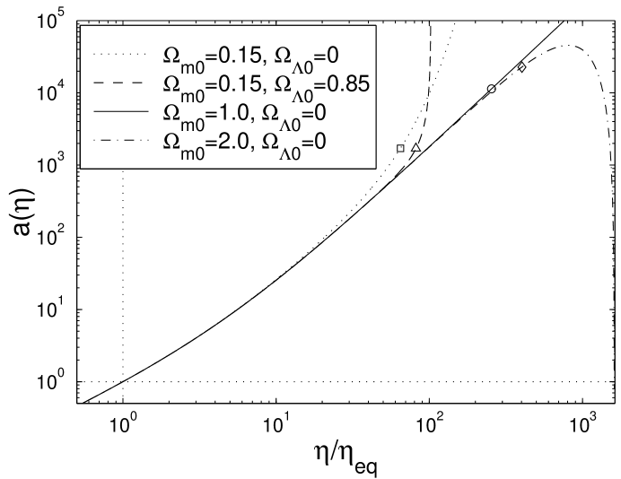
Figure A.1: The effect of the curvature and the cosmological constant in the background cosmology. Plotted are the exact solutions of scale factor $a(\eta)$ (see text for details). The square, triangle, circle and diamond mark the epoch today (with $h=0.7$) for different models.

Appendix B. Power Spectrum Conventions

We define the Fourier transform as:

$$\widetilde{f}({\bf k})=\frac{1}{V}\int d^{3}{\bf x}f({\bf x})e^{i{\bf k\cdot x}}\,,$$ (B.1)

where ${\bf k}$ is the wave vector, ${\bf x}$ the physical coordinates, and the integration taken over a large volume $V$. We will use a tilde $\;\widetilde{}\;$ to denote the Fourier transform of a function. The power spectrum ${\cal P}(k)$ for a mass density distribution $\rho({\bf x})$ is then defined as the spherically symmetric Fourier transform of the autocorrelation function $\xi(r)$ of density contrast $\delta({\bf x})=\delta\rho/\rho_{\rm av}$:

$${\cal P}(k)=\frac{1}{2\pi^{2}}\int\xi(r)\frac{\sin{kr}}{k}rdr={V\langle|\widetilde{\delta}_{\bf k}|^{2}\rangle\over 8\pi^{3}}\,,$$ (B.2)

where $k=|{\bf k}|$, $r$ is the correlation distance, and $\widetilde{\delta}_{\bf k}$ is the Fourier transform of the perturbations $\delta({\bf x})$. A useful quantity when comparing numerical results with observation is the dimensionless “spectrum of the matter density contrast”, which is given by contributions of $\widetilde{\delta}_{k}$ over a logarithmic interval $\triangle k/k\sim 1$:

$$S(k)=\left\langle\left(\frac{\delta\rho}{\rho_{\rm av}}\right)^{2}\right\rangle_{k}\approx\frac{Vk^{3}}{2\pi^{2}}\langle|\widetilde{\delta}_{k}|^{2}\rangle=4\pi k^{3}{\cal P}(k)\,.$$ (B.3)

This quantity is dimensionless and gives the rms density fluctuation on a particular length-scale $l=2\pi/k$. Another useful statistic is the mass fluctuation amplitude at certain length-scale $\lambda$, i.e. the standard deviation of the mass density distribution $\sigma_{\lambda}$. We convolve the density contrast $\delta({\bf x})$ with a spherical window of radius $\lambda$ to obtain the variance:

$$\sigma_{\lambda}^{2}=4\pi\int|w(k\lambda)|^{2}k^{2}{\cal P}(k)dk\;\;{\rm with}\;\;w(x)=\frac{3(\sin x-x\cos x)}{x^{3}}\,.$$ (B.4)

We note that $w(x)$ is the Fourier transform of a spherical window and ${\cal P}(k)$ in (B.4) can be calculated from (B.2).

References

- [1] J. R. Bond and G. Efstathiou, Ap. J. 285, L45 (1984).
- [2] G. Efstathiou, in Physics of the Early Universe, edited by A. Heavens, A. Davies and J. Peacock (Scottish Universities Summer School Publications, Edinburgh, 1990).
- [3] A. R. Liddle and D. H. Lyth, Phys. Rep. 231, 1 (1993).
- [4] For a review see A. Vilenkin and E. P. S. Shellard, Cosmic strings and other topological defects (Cambridge University Press, 1994)..
- [5] U. L. Pen, U. Seljak, and N. Turok, Phys. Rev. Lett., 79, 1615 (1997).
- [6] P. P. Avelino, E. P. S. Shellard, J. H. P. Wu, and B. Allen, Phys. Rev. Lett. 81, 2008 (1998).
- [7] P. P. Avelino, E. P. S. Shellard, J. H. P. Wu, and B. Allen, Ap. J. Lett. 507, L101 (1998).
- [8] P. P. Avelino, E. P. S. Shellard, J. H. P. Wu, and B. Allen, Phys. Rev. D 60, 023511 (1999).
- [9] P. P. Avelino, R. R. Caldwell, and C. J. A. P. Martins Phys. Rev. D 56, 4568 (1997).
- [10] A. Albrecht, R. A. Battye, and J. Robinson, Phys. Rev. Lett. 79, 4736 (1997).
- [11] R. A. Battye, J. Robinson, and A. Albrecht, Phys. Rev. Lett. 80, 4847 (1998).
- [12] B. Allen, R. R. Caldwell, S. Dodelson, L. Knox, E. P. S. Shellard, and A. Stebbins, Phys. Rev. Lett. 79, 2624 (1997).
- [13] C. Contaldi, M. Hindmarsh & J. Magueijo, Phys. Rev. Lett. 82, 679 (1999).
- [14] B. Allen and E. P. S. Shellard, Phys. Rev. Lett. 64, 119 (1990); B. Allen and E. P. S. Shellard, Phys. Rev. Lett. 64, 685 (1990); E. P. S. Shellard and B. Allen, “On the Evolution of Cosmic Strings” in The Formation and Evolution of Cosmic Strings (Cambridge University Press: Cambridge) (1990).
- [15] S. Veeraraghavan and A. Stebbins, Ap. J. 365, 37 (1990). Note that equations (5.42) and (5.46a) are incorrect, because they used wrong initial conditions. A complete set of corrected solutions are provided in Ref.?.
- [16] J. H. P. Wu, in preparation (2000).
- [17] J. R. Bond and G. Efstathiou, Ap. J. 285, L45 (1984).
- [18] U. Seljak and M. Zaldarriaga, Ap. J. 469, 437 (1996).
- [19] A. Stebbins, “A New Picture for Cosmic String seeded structure formation” in The Formation and Evolution of Cosmic Strings (Cambridge University Press: Cambridge) (1990).
- [20] D. P. Bennett and F. R. Bouchet, Phys. Rev. D41, 2408 (1990).
- [21] D. P. Bennett, “High Resolution Simulations of Cosmic String Evolution: Numerics and Long String Evolution” (1990); F. R. Bouchet, “High Resolution Simulations of Cosmic String Evolution: Small Scale Structure and Loops” in The Formation and Evolution of Cosmic Strings (Cambridge University Press: Cambridge) (1990).
- [22] J. V. Villumsen, Ap. J. Suppl. Ser. 71, 407 (1989).
- [23] A. Albrecht, R. A. Battye and J. Robinson, Phys. Rev. D 59, 023508 (1999).
- [24] J. H. P. Wu, P. P. Avelino, E. P. S. Shellard and B. Allen, in preparation.
- [25] A. Vilenkin, Phys. Rev. Lett. 46, 1169 (1981).
- [26] J. Silk and A. Vilenkin, Phys. Rev. Lett. 53, 1700 (1984); Ya. B. Zel’dovich,Mon. Not. R. Astron. Soc.192, 663 (1980).
- [27] D. P. Bennett and F. R. Bouchet, Phys. Rev. D 41, 2408 (1990).
- [28] R. Basu, A.H. Guth, & A. Vilenkin, Phys. Rev. D44, 340 (1991). J. Borrill, Phys. Rev. Lett. 76, 3255 (1996). E. J. Copeland, T. W. B. Kibble & D. A. Steer, Phys. Rev. D 58, 43508 (1998).
- [29] R. J. Scherrer, J. M. Quashnock, D. N. Spergel and W. H. Press Phys. Rev. D 39, 371 (1989).
- [30] B. Allen, E. P. S. Shellard Phys. Rev. D 45, 1898 (1992).
- [31] T. Vachaspati, A. Vilenkin Phys. Rev. D 31, 3052 (1985).
- [32] A. Albrecht and A. Stebbins, Phys. Rev. Lett. 68, 2121 (1992).
- [33] C. Cheung and J. Magueijo, Phys. Rev. D 56, 1982 (1997).
- [34] P. P. Avelino, E. P. S. Shellard, J. H. P. Wu, and B. Allen, work in progress.
- [35] A. Albrecht and A. Stebbins, Phys. Rev. Lett. 69, 2615 (1992).
- [36] A. Jenkins, C. S. Frenk, F. R. Pearce, P. A. Thomas, J. M. Colberg, S. D. M. White, H. M. P. Couchman, J. A. Peacock, G. Efstathiou, and A. H. Nelson, Ap. J. 499, 20 (1998).
- [37] A. R. Liddle, D. H. Lyth, D. Roberts, and P. T. P. Viana, Mon. Not. R. Astron. Soc. 278, 644 (1996).
- [38] S. M. Carroll, W. H. Press, E. L. Turner, Annu. Rev. Astron. Astrophys. 30, 499 (1992).
- [39] D. J. Eisenstein, Astro-ph/9709054 (1997).
- [40] P. P. Avelino and J. P. M. de Carvalho, Mon. Not. R. Astron. Soc. 310, 1170 (1999).
- [41] J. A. Peacock and S. J. Dodds, Mon. Not. R. Astron. Soc. 267, 1020 (1994).
- [42] A. J. S. Hamilton, M. Tegmark and N. Padmanabhan, Mon. Not. R. Astron. Soc. 317, L23 (2000).
- [43] J. Einasto et al., Ap. J. 519, 441 (1999).
- [44] J. P. Henry, ApJ, in press, Astro-ph/0002365 (2000).
- [45] J. H. P. Wu, Astro-ph/0012207 (2000).
- [46] A. Sornborger, R. Brandenberger, B. Fryxell, and K. Olson, “The Structure of Cosmic String Wakes”, Proceedings for 18th Texas Symposium on Relativistic Astrophysics; Astro-ph/9704145 (1997).
- [47] P. T. P. Viana and A. R. Liddle, Mon. Not. R. Astron. Soc. 281, 323 (1996).
- [48] V. R. Eke, S. Cole, and C. S. Frenk, Mon. Not. R. Astron. Soc. 282, 263 (1996).
- [49] S. D. M. White, G. Efstathiou, C. S. Frenk, Mon. Not. R. Astron. Soc. 262, 1023 (1993).
- [50] B. Allen, R. R. Caldwell, E. P. S. Shellard, A. Stebbins and S. Veeraraghavan, Phys. Rev. Lett. 77, 3061 (1996).
- [51] P. P. Avelino, R. R. Caldwell Phys. Rev. D 53, 5339 (1996).
- [52] S. Hanany et al., Ap. J. Lett. 545, L5 (2000).
- [53] P. de Bernardis et al., Nature 404, 955 (2000).
- [54] A. H. Jaffe et al., Phys. Rev. Lett., accepted (2001).
- [55] F. R. Bouchet, P. Peter, A. Riazuelo and M. Sakellariadou, Astro-ph/0005022 (2000).