Mass and Metallicity of Five X-ray Bright Galaxy Groups

Abstract

We present ASCA X-ray observations of a sample of five groups selected from a cross-correlation of the ROSAT All-Sky Survey with the White et al. optical catalog of groups. These X-ray bright groups significantly increase the number of known systems with temperatures between 2 and 3 keV. They have element abundances of roughly 0.3$\odot$ that are typical of clusters, but their favored ratio of Si/Fe abundance is lower than the cluster value. Combining the ASCA results with ROSAT imaging data, we calculate total masses of a few to several times $10^{13}\ {\rm M}_{\odot}$, gas mass fractions of $\sim$10%, and baryonic mass fractions of at least 15$-$20% within a radius of 0.5 Mpc. Upper limits for the ratios of gas to galaxy mass and of the iron mass to galaxy luminosity overlap with the range observed in rich clusters and extend to lower values, but not to such low values as seen in much poorer groups. These results support the idea that groups, unlike clusters, are subject to the loss of their primordial and processed gas, and show that this transition occurs at the mass scale of the 2$-$3 keV groups. A discussion of ASCA calibration issues and a comparison of ROSAT and ASCA temperatures are included in an Appendix.

1 Introduction

A group with few galaxy members can be readily identified as a gravitationally bound system rather than a chance superposition of galaxies on the sky through the detection of X-ray emitting intragroup gas. Pointed observations with the Einstein and ROSAT X-ray Observatories have by now identified several dozen X-ray emitting groups (e.g., Kriss et al. 1983, Price et al. 1991, Pildis et al. 1995, Henry et al. 1995, Doe et al. 1995, Mulchaey et al. 1996, Ponman et al. 1996). Results using spectrometers of higher resolution and bandwidth on the ASCA Observatory have now been presented by Fukazawa et al. (1996), Pedersen et al. (1997), and Davis et al. (1998), among others. Given that groups are the most common environment for galaxies, but are poorly understood compared to their richer cluster cousins, it is important to enlarge the sample of X-ray emitting groups that have been well-studied. The ROSAT All-Sky X-ray Survey (RASS) is expected to best identify those groups with the highest fluxes, while ROSAT’s limited spectral resolution and bandwidth make data obtained by ASCA better suited for a spectral study.

In this paper, we present X-ray data from the ASCA Observatory for five groups of galaxies (N56-395, S34-111, S49-132, N34-175, and S49-140) selected from a cross-correlation of the RASS with an optically-selected catalog of groups compiled by White et al. (WBL, 1998; the corresponding WBL catalog numbers are, respectively, WBL518, WBL025, WBL698, WBL636, and WBL061). The White et al. catalog was constructed from the Zwicky catalog of galaxies by an automated process that mimics the criteria used to create the MKW and AWM catalogs. The cross-correlation with the RASS, which provided 98% coverage of the X-ray sky at energies from 0.1 to 2.0 keV, was carried out on a subsample of 68 of the more than 700 groups in the catalog (Burns et al. 1996). Our groups are those with the highest X-ray flux that are also of sufficiently small angular size that the ASCA instruments (in particular, the SIS in 2-CCD mode) intercept most of their flux. These groups should be among the X-ray brightest in the northern sky.

Our X-ray bright groups have higher temperatures and luminosities and correspondingly higher masses than the very poor, low temperatures systems that have been more widely studied. The low temperature groups show a wide dispersion in their element abundance and in their distribution of mass among gas, galaxies, and dark matter. This has led to the suggestion that groups are at the threshold to bind their primordial and processed gas (Fukazawa et al. 1996, Renzini 1997). We can test this idea for a somewhat higher mass and temperature range with our sample of groups. Throughout this paper, we use $H_{0}=50$ km/s/Mpc.

2 Data Analysis

To calculate the mass in various components of the groups, we require both X-ray spectral and imaging measurements, and optical galaxy luminosities. X-ray spectral data from the ASCA Observatory are used to measure the temperatures and element abundances of the hot X-ray emitting gas, and to place constraints on the variation of these quantities with radius. Imaging data from ROSAT as well as ASCA are used to characterize the X-ray surface brightness profiles of the hot gas and to infer the density distributions. Optical galaxy luminosities are used to estimate the mass contained in the group galaxies. Here we describe the reduction of the X-ray data and review the optical properties of the groups.

2.1 Data Reduction

Data for the groups were obtained with the instruments on the ASCA Observatory in 1996 and 1998. The ASCA satellite and its instruments are described by Tanaka et al. (1994). Here we briefly note that ASCA has two Solid-State Imaging Spectrometers (SIS0 and SIS1) and two Gas Imaging Spectrometers (GIS2 and GIS3), with slightly offset fields of view. Each instrument has its own telescope with nested conical foil mirrors that provide a point-spread function (PSF) with a narrow core of about $1^{\prime}$ FWHM, and a half-power diameter of $3^{\prime}$. The GIS broadens the PSF further. The SIS are square arrays of four CCD chips that can be used with 1, 2, or all 4 of the chips exposed simultaneously. Observations of extended sources are now carried out primarily in 2-CCD mode because of declining instrument performance in 4-CCD mode. The field of view of the SIS in 2 CCD mode is $11^{\prime}\times 22^{\prime}$. The GIS field of view is significantly larger ($40^{\prime}$ useful diameter), but the GIS provides data of lower spectral and spatial resolution than does the SIS. The data were screened and processed following standard data reduction procedures as outlined in the ASCA ABC Guide (Day et al., 1997). Further details on the data processing can be found in the Appendix. Table 1 lists the ASCA observations including the GIS2 exposure time. We also give the source coordinates from Ledlow et al. (1996), the nominal Galactic neutral H column density from Dickey & Lockman (1990), the group redshift, and the exposure of available X-ray data from the ROSAT PSPC.

All the groups except N56-395 were also observed by the Position Sensitive Proportional Counter (PSPC) on the ROSAT Observatory. The PSPC provided excellent imaging of 0.2 to 2 keV X-rays combined with low resolution spectroscopy. We use software developed by Snowden et al. (1994) to produce appropriate energy-dependent exposure maps and to model and subtract the particle background and contamination by scattered solar X-rays and by the so-called long-term enhancements (the reader is referred to Snowden et al. for a discussion of these effects). The data for S49-132 and S49-140 have also been analyzed by Doe et al. (1995) as a part of a sample of groups with extended radio sources, and those for S34-111 (3C31) by Trussoni et al. (1997). The ROSAT High Resolution Imager data for S34-111 are presented by Trussoni et al.; we briefly discuss the 2.1 ks HRI observation of N34-175 in Section 2.4.

2.2 ASCA Spectra

For each group, a circular region on the sky containing most of the counts was chosen for spectral analysis by examining the GIS image. These regions generally did not fit completely within the SIS field of view. Background spectra were taken from the same detector region on averaged blank sky fields provided by the ASCA Guest Observer Facility. Typically, the individual SIS and GIS spectra had $>$3000 counts after subtraction of the background, but those of S49-140 had only 900$-$1400 counts, partly because of the exclusive use of FAINT mode data. Calibration data from February 1996 and March 1997 were used to create appropriate instrument response files for each pulse height spectrum.

Spectra from all four ASCA detectors were fitted simultaneously to the same spectral model with the relative normalizations allowed to be fitted freely for each detector. We use Raymond & Smith optically thin thermal models (1977 as updated in XSPECv10.0; hereafter RS) with the abundances of elements heavier than He taken to be in solar abundance ratios from Anders & Grevesse (1989). The column densities of SIS0 and SIS1 were allowed to be different from each other, and were fitted freely, while the column densities for GIS2 and GIS3 were fixed at the Galactic value (see the Appendix). Figure 1 shows the global ASCA spectral data for each instrument overlaid with the best-fit model folded through each instrument response. Table 2 summarizes the results of these spectral fits. The errors given in this and subsequent tables are for 90% confidence. The temperatures are typically 2$-$3 keV, and the gas metallicities are roughly 0.3 $\odot$. The column densities of SIS0 are listed only for completeness; they are certainly over-estimated for all but N56-395 (see the Appendix). The emission measures given are for GIS2; the GIS3 values are consistent with these to well within 10%, whereas the SIS is not useful for obtaining the emission measure because of its limited field of view. For N56-395, part of the 12^′ radius region used falls outside the useful radius of the GIS; we applied geometrical correction factors for the emission measure of 1.17 for r = $4.5^{\prime}-12^{\prime}$ and 1.14 for r$<12^{\prime}$.

We then divided each group into two annular regions to constrain radial variations in the temperature and abundance. The width of the annuli are constrained both by the spatial resolution of the ASCA mirrors and by the requirement that each spectrum have a sufficient number of source counts ($\sim 1000$). Strictly, a spatially resolved analysis of the ASCA spectrum should account for the broad and energy-dependent point-spread function (PSF). The relatively low temperature of our groups reduces the need for this, as spurious spatial trends arising from neglect of the PSF are shown to be small for temperatures below about 3 keV (Takahashi et al. 1995, ASCA News, 3, 34). As shown in Table 2, isothermal temperatures and constant element abundances are fully consistent with this analysis. Results for S49-140 are not shown in this table, but are also consistent with isothermal temperatures and constant abundances.

To place constraints on the relative abundances of the elements, we fitted the integrated spectrum with a model in which the abundances of C, N, O, Ne, and Mg are fixed at 0.3 $\odot$, the abundances of Si, S, Ar and Ca tied to each other in their solar ratios, and Fe tied to Ni. We thereby obtain a measurement of the relative abundance of intermediate mass elements represented by Si compared to Fe. This ratio is a diagnostic of the enrichment process in the hot gas. The results of our fits are shown in Table 3. All the groups have a ratio of Si/Fe abundance that is consistent with the solar value. Contour plots of the Si abundance vs. the Fe abundance are shown for N56-395 and S34-111 in Figure 2. A ratio of the Si/Fe abundance that is twice the solar value falls outside the 99% and 90% confidence contours, respectively, for these two groups.

2.3 Discussion of Spectral Fits

The robustness of the spectral results can be assessed by comparing them to the results of fitting each detector individually, since the simultaneous fitting tends to average out the calibration errors for individual detectors and give relatively tight errors for the fitted parameters. The fitted temperatures typically vary by about 10% between the individual detectors with two exceptions. For S34-111, the 20% consistency probably results because, unlike the GIS, the SIS does not include all the X-ray emitting galaxies in its field of view. For the outer region of S49-132, a 1$-$2 keV difference between the SIS and GIS temperatures evidently arises from residual high energy features in the SIS spectrum. The SIS temperatures are consistent with the GIS temperatures when this portion of the spectrum is ignored, and the joint SIS and GIS fits favor a temperature near the GIS value.

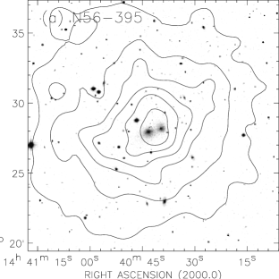
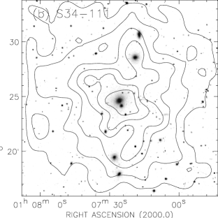
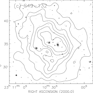
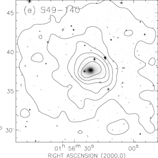
Figure 3: X-ray contours from ASCA GIS 2 images overlaid on Palomar Survey optical images. Each region shown is 18^′ across. The X-ray images have been smoothed with a Gaussian function with $\sigma=0.6^{\prime}$. The contours are linearly spaced. For N56-395, the minimum and maximum contours correspond to 4.8$\times 10^{-4}$ and 2.4$\times 10^{-3}$ counts/s/arcmin²; for S34-111, these contours correspond to 3.4$\times 10^{-4}$ and 1.1$\times 10^{-3}$; for S49-132, 4.8$\times 10^{-4}$ and 1.6$\times 10^{-3}$; for N34-175, 1.1$\times 10^{-3}$ and 6.7$\times 10^{-3}$; for S49-140, 2.2$\times 10^{-4}$ and 1.1$\times 10^{-3}$.

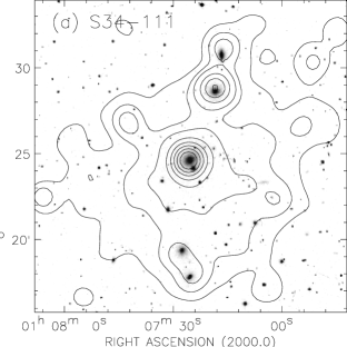
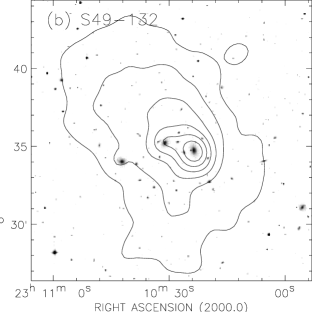
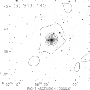
Figure 4: X-ray contours from ROSAT PSPC 0.5-2.0 keV images overlaid on the same optical images as in Figure 3. The ROSAT contours for S34-111 are linearly spaced between 0.001 to 0.007 counts/s/arcmin², with an additional contour (the second lowest) at 0.0015; for S49-132, between 0.0012 and 0.0069; for N34-175, between 0.002 and 0.045, plus an additional contour (the second lowest) at 0.005; for S49-140, between 0.008 and 0.011.

The single-temperature thermal model that we use is the simplest possible description of the group X-ray emission consistent with the ASCA data. A number of galaxies are detected as X-ray sources, as seen in Figures 3 and 4. In addition, some of these galaxies are also radio sources: N34-175 has a compact radio source associated with the central galaxy NGC 6338 (e.g., Gregory & Condon 1991), and may have nonthermal X-ray emission associated with it as discussed below; the central galaxy in S34-111, NGC 383, is the radio source 3C31 (see Trussoni et al. 1997 and references therein); southeast of the center of S49-132, the galaxy NGC 7503 is an extended radio source with a head-tail morphology, while the central galaxy in S49-140, NGC 742, is a head-tail radio source (possibly together with NGC 741; see Doe et al. 1995 and references therein).

We therefore tried adding a power-law component (presumably emission from an active galactic nucleus) to the spectral model for each group. We used a fixed energy index of 1.7 and fixed the column densities at their values in the fits listed in Table 2. We found that the fits for all the groups could be improved in this way, but N34-175 was the only group for which there was both a significant improvement in the fit statistic and a significant change in the fitted temperature (see Tables 2 and 3). The normalizations of the power-law component in the two radial annuli are nearly equal, however, whereas the normalization of the inner annulus should be twice higher if the power-law component originates from a point-source at the center. The uncertainties in the normalizations do not rule out a point-source origin from an AGN, but it is difficult to rule out the possibility that at least some of the power-law is a coincidental compensation for residual calibration deficiencies. We list results for both a pure thermal spectrum and for the addition of a power-law for N34-175 throughout. The 0.5$-$10 keV luminosity of the power-law component is about 2$\times 10^{43}$ ergs/s. The relative abundance of Si to Fe increases to 1.5 times the solar value, but is still consistent with the solar value. The group S49-140 is also dominated by its central galaxy, but here the 90% upper limit on the 0.5$-$10 keV power-law luminosity is only about 6 $\times 10^{41}$ ergs/s.

2.4 X-ray Images

Figure 3 shows the Palomar optical survey image of a $18^{\prime}$ square region centered on each group with the ASCA GIS2 X-ray contours overlaid. Figure 4 shows the same Palomar images overlaid with the ROSAT PSPC X-ray contours in the approximate energy range 0.5 to 2.0 keV. There are no PSPC data for N56-395. The X-ray images in both figures were smoothed with Gaussian $\sigma=0.6^{\prime}$ and shifted slightly to align them with the optical images. Only S49-132 is markedly elongated in X-rays, with the elongation following the galaxy distribution (Doe et al. 1995). The groups N34-175 and S49-140 are dominated by their central galaxies.

It is preferable to use the ROSAT PSPC images to characterize the surface brightness profile of the diffuse X-ray emission because the ROSAT point-spread-function (PSF) has FWHM=25^′′ at energy 1 keV while the ASCA mirrors have a broader and more complex spatial response. As noted, ROSAT data are available for all the groups except N56-395. For S34-111 and S49-132, we mask out the sources from the 0.5$-$2.0 keV images to form radial surface brightness profiles of the diffuse emission. We use 1^′ bins centered at a position determined by eye out to a radius of about 50^′. The profile of the diffuse emission is fitted with a King isothermal model for the surface brightness $\sigma$ as a function of radius $r$:

$$\sigma(r)=\sigma_{0}\ \left(1+\left(\frac{r}{r_{c}}\right)^{2}\right)^{-3\beta+\frac{1}{2}}+B_{0},$$

where $\beta$ is the slope parameter, $r_{c}$ the core radius, $\sigma_{o}$ the normalization, and $B_{0}$ a constant background. The 1 keV ROSAT PSF is convolved with the model, but the results are not very sensitive to the exact PSF used. In N34-175 and S49-140, the central galaxy is particularly bright so it is included in the profile and modelled as an additional gaussian component. Other sources are removed, and 0.5^′ bins are used. The radial profiles are shown in Figure 5, along with the ROSAT HRI profile of N34-175, and the fit parameters are summarized in Table 4.

Since N56-395 was not observed with the PSPC, we use the ASCA GIS images to constrain the shape of its surface brightness profile. We do not attempt to subtract out the emission from individual sources because of the extent of the ASCA PSF (the telescope gives a $1^{\prime}$ core and half-power diameter of $3^{\prime}$ and the GIS increases this). We generate the appropriate spectrally weighted PSF at the pointing center by using the GIS pulse-height spectrum as input to a ray-tracing program. The fit results are summarized in Table 4 and Figure 5. The reliability of the ASCA surface brightness fits for N56-395 can be tested by comparing such fits for the other groups against the ROSAT results. We find good agreement provided that point sources do not make a large contribution to the flux. The results for N56-395 should be fairly reliable since the ROSAT PSPC All-Sky Survey image of N56-395 does not show strong point sources (Burns et al. 1996).

From their analysis of ROSAT data, Doe et al. (1995) obtained results ($\beta=0.58\pm 0.10$ and $r_{c}=5.0^{\prime}\pm 0.2^{\prime}$) in good agreement with ours for S49-132 . Their values for S49-140 ($\beta=0.60\pm 0.20$ and $r_{c}=4.4^{\prime}\pm 0.4^{\prime}$) are higher than ours, possibly because they simply exclude the innermost radial bin, whereas we fitted both the diffuse and the galaxy components in the surface brightness profile. Trussoni et al. (1997) use different software and obtain higher values ($\beta=0.61\pm 0.06$ and $r_{c}=7.7^{\prime}\pm 1^{\prime}$) than we do for S34-111, but Price et al. (1991) use limited quality Einstein data to obtain values ($\beta=0.4-0.5$ and $r_{c}=0.8^{\prime}-2.5^{\prime}$) similar to ours.

N56-395 and S34-111 have low fitted values of $\beta\sim$0.4 that are indicative of relatively flat surface brightness profiles. The flatness of S34-111 relative to S49-132, for example, is evident in Figure 5. However, the model-fitting carried out here assumes spherical symmetry, and all the groups show some sign of departure from spherical symmetry. The assumption of spherical symmetry for an elongated gas distribution may result in spuriously low values of $\beta$ (Makishima et al. 1995), although the most obviously elongated of our groups (S49-132) actually has the highest fitted value of $\beta$. A more complex, two-component profile can also be mimicked by a single flat profile (Mulchaey & Zabludoff 1998).

2.5 Optical Data

Optically measured velocity dispersions, two-point correlation coefficients, and luminosities for the group galaxies are summarized in Table 5. The velocity dispersions $\sigma$ are the quantity $S_{BI}$ calculated at 0.75 Mpc from Ledlow et al. (1996) except for S49-132, for which it is calculated in the conventional way using velocity and position data in Ledlow et al. for galaxies within a 0.75 Mpc radius circle. For most of the groups, the velocity dispersions are based on fewer than 20 or even 10 galaxies, and the true dispersion may actually lie outside the formal errors. Zabludoff & Mulchaey (1998) show from their deep optical spectroscopic measurements that velocity dispersions calculated using only the brightest galaxies tend to significantly underestimate the true dispersion. In addition, some of the groups are embedded in larger systems or are interacting with nearby systems, making the velocity data difficult to interpret. For example, S49-132 is embedded in a larger Zwicky cluster and has an exceptionally high velocity dispersion. Its velocity distribution is noted by Ledlow et al. (1996) and Doe et al. (1995) to be unusually broad and flat, with three of the central galaxies separated by 1000 km/s in velocity. N56-395 (MKW 8) is probably interacting with the nearby group MKW 7 (Beers et al. 1995) and its velocity dispersion calculated to 1.5 Mpc increases substantially to 422${}^{+99}_{-53}$ km/s.

The two-point galaxy-galaxy correlation coefficient $B_{gg}$ (see Andersen & Owen 1995) is calculated for N galaxies over an angular scale $\theta$ chosen to optimize signal-to-noise. It directly reflects the galaxy richness of the group, and correlates with both the X-ray luminosity and gas temperature. S49-132 has the highest value of B_gg among our groups, while N34-175 and S49-140 both have low B_gg.

The estimated optical galaxy luminosities are based on B band magnitudes from the Third Reference Catalog of Bright Galaxies (3RC; de Vaucouleurs et al. 1991) as accessed through HEASARC and NED. Wherever available, these are the extrapolated, extinction and redshift corrected blue magnitudes (B${}_{\rm T}^{0}$). We include group galaxies that are located within the radius used for the X-ray spectral fits, which turns out to be nearly the same as for a uniform physical radius of 0.5 Mpc. We do not attempt a correction for faint, undetected galaxies, and magnitudes are not yet available for many of the fainter galaxies in the redshift compilation of Ledlow et al., so our tabulated luminosities are lower limits.

3 Results

We now examine physical measurements derived from the data: the X-ray luminosity and its relationship to the X-ray temperature and to optically measured dynamical properties; the distribution of mass between the gas, galaxy, and dark matter components; and the abundances of the elements. These are compared to measurements for other groups (most at lower temperatures than ours) and to rich clusters to test if our hotter groups provide a transition between these systems.

3.1 X-ray Luminosities

We list in Table 6 the 0.5$-$10 keV X-ray source luminosities measured within the radii used for the spectral fits. The luminosities can be scaled to other radii by using the results of the surface brightness profile fits. We also give luminosities at a fixed physical radius of 0.5 Mpc and at a radius representative of the extent of the X-ray emission. We define this extent to be the radius where the surface brightness profile falls to 2% of its peak value. The multiplicative correction factors at these radii are 1.6 at 22^′ (1 Mpc) for N56-395, 5.2 at 64^′ (1.9 Mpc) for S34-111, 1.6 at 20^′ (1.5 Mpc) for S49-132, 1.3 at 12^′ (0.6 Mpc) for N34-175, and 2.4 at 24^′ (0.8 Mpc) for S49-140.

The X-ray luminosities and temperatures of the groups appear to be consistent with the well-known correlation in clusters (e.g., Mushotzky 1984, Edge & Stewart 1991, David et al. 1993, Mushotzky & Scharf 1997, Fukazawa 1997). In Figure 6 we show the 0.5$-$10 keV X-ray luminosity $L_{X}$ at 0.5 Mpc against the X-ray temperature $kT$ of our groups (square points) compared to a sample of clusters and groups studied with ASCA by Fukazawa (1997). The groups fall on the lower luminosity end of the relation defined by the clusters. At temperatures kT $\lesssim$ 1 keV, Ponman et al. (1996) use ROSAT data for compact groups and find a steeper correlation that they suggest may arise from the action of galactic winds. Mulchaey & Zabludoff (1998), however, find no evidence for such steepening in their sample of low temperature (kT $<$ 1 keV) groups.

The X-ray luminosities and various optical measures of the group richness also appear to follow the same trends seen in richer clusters. For example, a strong correlation exists between $L_{X}$ and the optical velocity dispersion $\sigma$ in rich clusters (Quintana & Melnick 1982, Edge & Stewart 1991b). Price et al. (1991) used Einstein Observatory X-ray data to show that poor clusters and groups extend the relation found for richer clusters. The issue has been complicated since then as Dell’Antonio et al. (1994) and Mahdavi et al. (1997) suggest that the relation flattens for lower luminosity groups as the galaxy luminosities begin to dominate over that of the intragroup gas. If the galaxy emission is excluded, however, the cluster $L_{X}-\sigma$ relation appears to hold for the intragroup gas (Ponman et al. 1996, Mulchaey & Zabludoff 1998). Our groups generally follow the cluster relation, with the possible exception of N56-395, for which the velocity dispersion listed in Table 5 is somewhat low relative to the X-ray temperature and luminosity. If the higher dispersion calculated at 1.5 Mpc by Beers et al. (1995) is used for N56-395, there is better agreement with the average cluster relation. Our groups also fall within the range of other clusters and groups for the relationship between the X-ray luminosity and the two-point galaxy correlation coefficient B_gg shown by Doe et al. (1995). The one strong exception is N34-175, for which B_gg is markedly low for its X-ray luminosity. This persists even if the lower luminosity from the model including a component for the AGN is adopted. The relative sparseness of galaxies in this group, which is reflected in the low value of B_gg, can be seen in Figures 3 and 4. N34-175 otherwise shows no anomalies and, as will be shown in the following section, shows no peculiarities in its mass or baryon fraction.

With the exceptions noted above, the relations for the X-ray luminosity to X-ray temperature and to optical richness seen in the richer clusters appear to hold at the lower mass scales of the kT $\sim 2-3$ keV groups in our sample.

3.2 Masses and Mass Ratios

The mass contained in galaxies, gas, and dark matter in the groups may be calculated with a few standard assumptions. The mass of the galaxies can be estimated from the galaxy luminosities by assuming a mass-to-light ratio for each galaxy, while the mass of the X-ray emitting gas and the total gravitational binding mass can be computed from the X-ray spectral and imaging results by assuming that the gas is spherically symmetric and in hydrostatic equilibrium. The distribution of mass between the various components is then easily seen by taking ratios of the masses. These masses and mass ratios are tabulated in Table 7 both at the radii used for the ASCA fits and at a fixed physical radius of 0.5 Mpc.

To calculate the mass of a galaxy from its optical B-band luminosity, an appropriate mass-to-light ratio (M/L) must be determined for it depending on its galaxy type. Most of the galaxies are E or S0; for those with published velocity dispersions and effective (half-light) radii, we calculate M/L using the scaling in the Fundamental Plane for elliptical galaxies based on Loewenstein & White (1998). Galaxy velocity dispersions are taken from McElroy (1995), and effective radii from 3RC. For galaxies with magnitude information only, we calculate M/L assuming the mean relation in the Fundamental Plane. A few faint (m${}_{\rm B}>$ 15) galaxies without morphological classifications are also treated as ellipticals. The M/L values are typically between 4 and 10 in solar units, with a few beyond either end. The groups S49-132 and S49-140 each have one relatively bright galaxy that dominates the mass because of a high M/L ratio arising from a large effective radius. If M/L for these galaxies is calculated from just the luminosity and the mean Fundamental Plane relation, the total galaxy masses in the lower part of Table 7 decrease from 7.9 to 6.2 $\times 10^{12}$ M_⊙ for S49-132, and from 4.2 to 2.9 $\times 10^{12}$ M_⊙ for S49-140. For the spiral galaxies, we use the mass-to-light relation given by Persic, Salucci, & Stel (1996), which scales with luminosity. The typical value of M/L for our spirals is $\sim 3$ in solar units. The galaxy masses in these groups range from 2 to 8 $\times 10^{12}\ {\rm M}{{}_{\odot}}$. These are lower limits because optical magnitudes are not available for many of the known group galaxies and no correction is attempted for them.

The gas mass is obtained by integrating the hydrogen density over the appropriate volume and assuming a mean mass per proton of 1.4 amu. The density in a King isothermal model with slope $\beta$ and core radius $r_{c}$ is given by

$$n(r)=n_{0}\ \left(1+\left(\frac{r}{r_{c}}\right)^{2}\right)^{-\frac{3}{2}\beta}.$$

The central density $n_{0}$ is determined by equating the spectrally fitted emission measure with the quantity $\frac{\int{n_{e}(r)n_{H}(r)dV}}{4\pi d^{2}}$, where the integral is over the emitting volume, $d$ is the distance to the source, and $n_{e}/n_{H}$ is taken to be 1.23. The central electron densities are given in Table 4. The gas masses at 0.5 Mpc are $(3-8)\times 10^{12}\ {\rm M}_{\odot}$, as given in Table 7.

The gravitational binding mass within a radius $r$ depends on the spatial gradients of the temperature $T$ and the density $\rho$:

$$M(<r)=\frac{-kT}{G\mu m_{p}}\ r\ \left(\frac{d\,{\rm ln}\rho}{d\,{\rm ln}r}+\frac{d\,{\rm ln}T}{d\,{\rm ln}r}\right)\,,$$

where k is Boltzmann’s constant, G is the gravitational constant, $m_{p}$ is the proton mass, and the mean mass per particle, $\mu$, is taken to be 0.6 amu. We assume that the gas is isothermal, since this is consistent with our spatially resolved spectral analysis (Table 2), and take the gas temperatures from the global spectral results in Table 2. Most groups for which the temperature profile has been measured are indeed consistent with being isothermal (e.g., see Mulchaey et al. 1996 and references therein, Fukazawa et al. 1996), with the exception of those whose central regions may harbor cooling flows (e.g., Fukazawa et al. 1996, 1996b, Ponman & Bertram 1993). The total binding masses at 0.5 Mpc for our groups are $(3-8)\times 10^{13}\ {\rm M}_{\odot}$ (Table 7), higher than those reported for lower temperature groups by Pildis et al. (1995) and Mulchaey et al. (1996), but comparable to those reported for six MKW and AWM poor clusters by Kriss et al. (1983) using Einstein Observatory data.

From the calculated masses, we can compare the distribution of the total mass between the various components: gas plus galaxy to total mass (baryon fraction), gas to total mass (gas fraction), and gas to galaxy mass. The only significant changes in these quantities between the ASCA radius and 0.5 Mpc radius are the gas mass fractions for S34-111 and S49-140. At the ASCA radius, which correponds to 0.3 Mpc for both, the gas mass fractions are 30% and 40% lower than at 0.5 Mpc.

The baryonic mass fractions of the groups range from 13 to 21% and overlap with much of the range for clusters, although some rich clusters have higher baryon fractions near 30%. The gas mass fractions are between 8 and 14% and are mostly near 10%, which is below the average value for clusters (Allen & Fabian 1998, White et al. 1997) but overlaps with the lower end of the cluster range. Some other groups, typically those with lower temperature gas, have gas mass fractions as low as 5% (e.g., Pedersen et al. 1997, Pildis et al. 1995, Mulchaey et al. 1996). At even lower mass scales, elliptical galaxies have gas mass fractions of less than 1% (Forman, Jones, & Tucker 1985). There is a progression of increasing gas mass fraction from elliptical galaxies to poorer groups to clusters, although it is not clear that this trend continues on cluster scales (e.g., White et al. 1997).

The upper limits for the ratio of gas mass to galaxy mass in our groups are between 0.6 and 3. In clusters, this ratio has been reported to be as high as 5$-$6 (Arnaud et al. 1992 at 3 Mpc, David et al. 1990 at 1 Mpc), but others report values of about 1$-$2 (Fukazawa 1997 at 1 Mpc, Edge & Stewart 1991 at 0.5 Mpc), and trends with mass on cluster scales are controversial. Ratios below 1 are reported for poorer groups (Mulchaey et al. 1996), with many compact groups having values $<$0.1 (Pildis et al. 1995); elliptical galaxies have ratios as low as $<$0.01 (Forman et al. 1985). There is clearly a large-scale trend of increasing M_gas/M_gal with mass from ellipticals to poor groups to clusters. The factor of 5 spread we find for our groups spans the range for rich clusters and goes significantly below it, showing that the deviations from the cluster values take place at this 2$-$3 keV mass scale. The values are significantly higher than the typical values for poorer groups, including the compact groups. The galaxy masses for the groups are lower limits, but it is unlikely that they are in error by substantially more than a factor of 2, and corrections to them will move the gas to galaxy mass ratios farther from the cluster values. Results in the literature are reported rather nonuniformly and there are few observations that extend to the virial radii of groups and clusters, but the large-scale trends noted here seem to be clearly established.

Errors in the gas mass due to the formal uncertainties in $\beta$ and $r_{c}$ and in $kT$ are typically smaller than a few percent, while the formal errors in the total mass are about 10% or less. N56-395 has the largest uncertainties in $\beta$ and $r_{c}$, and the error in its ratio of gas mass to total mass is about 13%. If we use the ROSAT results of Trussoni et al. (1997) for S34-111, with $\beta$ and $r_{c}$ about twice the values we obtain, the masses are still within about 10% of the values in Table 7. The systematic uncertainties in the mass calculations are likely to be comparable to or higher than the formal uncertainties. If the assumption of hydrostatic equilibrium does not hold, the mass calculations may be in error by some 30% (Evrard, Metzler, & Navarro 1996, Schindler 1996), and the neglect of an existing temperature gradient will contribute additional errors.

A simple check on our calculations for the total mass is to compare them to the virial mass derived from the scaling of mass and temperature in the simulations of Evrard, Metzler, & Navarro (1996). They provide analytical formulae depending only on the temperature of the X-ray emitting gas both for the virial radius, defined as enclosing a mass density contrast of 500 times the critical density, and for the corresponding mass. For 2 and 3 keV gas, these radii are 2.2 and 2.7 Mpc, and the masses are 2$\times 10^{14}\ {\rm M}_{\odot}$ and 3.65$\times 10^{14}\ {\rm M}_{\odot}$, respectively. Extrapolating our results to these radii, we derive masses that are in excellent agreement with the analytical predictions, with the exception of N34-175. Its extrapolated mass of 3$\times 10^{14}\ {\rm M}_{\odot}$ for a temperature near 2 keV is somewhat high. Using the lower 1.6 keV temperature from fitting an power-law component, the extrapolated mass of 2$\times 10^{14}\ {\rm M}_{\odot}$ is still high relative to the analytical mass of 1.4$\times 10^{14}\ {\rm M}_{\odot}$.

The gas mass obtained by Doe et al. (1995) for S49-132 is difficult to reconcile with ours. They process the ROSAT imaging data using methods similar to ours, and obtain $\beta$ and $r_{c}$ values in good agreement, but calculate the mass based on a deprojection of the ROSAT data. Much of the difference between our calculated gas masses is accounted for by their calculated central electron density being a factor of three higher than ours. The higher density would be required for the low ROSAT temperature of 2 keV they use compared to the ASCA temperature of 3 keV. At 0.5 Mpc, their X-ray luminosity is nearly an order of magnitude lower than ours, and their gas mass fraction of 45% is much higher than our value. For S49-140, our results are in reasonable agreement once the total mass is corrected for the ASCA temperature of 1.6 keV compared to the temperature 1.0 keV used by Doe et al., notwithstanding our discrepancies in $\beta$ and $r_{c}$.

3.3 Element Abundances

Our groups have average element abundances of about $0.3\odot$, which is the remarkably homogeneous value observed in the rich clusters (Allen & Fabian, 1998, Mushotzky et al. 1996 and references therein). Although some other groups have cluster-like abundances (e.g., Fukazawa et al. 1996), others have substantially lower element abundances (e.g., NGC 4261, Davis et al. 1995; NGC 2300, Davis et al. 1996). Low abundance groups have now been confirmed (NGC 2300, Sakima et al. 1995) and newly identified by ASCA (e.g., NGC 3259, Pedersen et al. 1997; also see Davis et al. 1998). Fukazawa (1997) and Renzini (1997) point out a pattern in the X-ray temperature and Fe abundance of groups and clusters: at temperatures above about 1 keV, the Fe abundance shows little variance from about 0.3 times solar, while at lower temperatures, there is a large spread in abundances, with a tendency toward very low values. Our groups fit into the pattern noted by Fukazawa and Renzini in that a 0.3 $\odot$ metallicity is expected for temperatures of 2$-$3 keV.

The Si/Fe abundance ratio in our groups favors the solar value, although a ratio of twice the solar value cannot in general be ruled out with more than 90% confidence. In other groups for which the Si/Fe abundance ratio has been determined so far, this ratio is generally about solar (Fukazawa et al. 1996, Davis et al. 1998). This is similar to the value determined for elliptical galaxies (Matsumoto et al. 1997), and lower than the value of twice solar characteristic of rich clusters (Mushotzky et al. 1996).

The quantity M_Fe/L_B is even more directly related to the stellar Fe yield than the abundances themselves (Arnaud et al. 1992). As shown in Table 7, the upper limits for our groups are between 0.005 and 0.015 in solar units when evaluated at a radius of 0.5 Mpc. Since this quantity is directly proportional to the Fe abundance, its errors are dominated by the uncertainties in the Fe abundance measurement. These errors range from less than 20% up to 45% in our groups (Table 2). The typical range of M_Fe/L_B in clusters is 0.01$-$0.02, measured at a radius of 3 Mpc, roughly the virial radius for clusters (Renzini 1997). Comparisons at different radii are a little risky, but the values for our groups are evidently at or below the typical range for clusters. In our sample, there appears to be a significant spread in this quantity ranging from the cluster value to below. The mass scale corresponding to temperatures of 2 to 3 keV is evidently that at which the M_Fe/L_B ratio begins to deviate from the cluster value. In the larger sample of Davis et al. (1998), two groups with temperatures $\sim$ 2 keV have even lower M_Fe/L${}_{\rm B}<$ 0.001. The pattern of increasing M_Fe/L_B in poor groups to rich clusters echoes that seen in the lower gas mass fractions and gas to galaxy mass ratios of groups compared to clusters.

4 Conclusions

Our study of a sample of five RASS-selected, X-ray bright groups shows that these objects have temperatures between 2 and 3 keV at the lower boundary of the temperature range for clusters. This is a temperature range for which relatively few objects have been well-studied thus far compared to those above and below it. Insofar as we are able to test the spatial temperature structure by comparing the spectra in two annular rings, it is consistent with being isothermal out to about 10^′. The temperatures and bolometric luminosities agree well with the relation established for richer clusters, reinforcing the conclusions of other authors that the bulk X-ray properties of groups are an extension of those of richer clusters (Price et al. 1991, Doe et al. 1995, Burns et al. 1996, Mulchaey & Zabludoff 1998). We also find that both the optically determined galaxy velocity dispersion and the galaxy richness parameter $B_{gg}$ compared to the X-ray luminosity generally agree well with the relations established by other clusters and groups. The dynamically complex group N56-395 has a relatively low velocity dispersion at 0.75 Mpc radius, whereas N34-175 has a low $B_{gg}$ for its X-ray luminosity.

The spectral and imaging data together allow estimates of the gas mass and the total gravitating mass in these systems. At a radius of 0.5 Mpc, the gas masses are a few to several times $10^{12}\ {\rm M}_{\odot}$, and the total masses are about a factor of ten higher, giving gas mass fractions near 10% for this sample. The ratio of mass in gas relative to that galaxies spans a factor of several and is no higher than about 0.6$-$3. These values overlap the range seen in clusters but are higher than those seen in lower temperature groups. Whereas poorer groups tend to have widely varying and often rather low abundances, our groups have element abundances typical of clusters, at roughly 0.3 $\odot$. The ratio of Si/Fe abundance, however, favors at 90% confidence a value near the solar ratio that is more characteristic of elliptical galaxies and poorer groups than of rich clusters. The ratio of Fe mass in the gas to the optical luminosity spans a factor of three range from 0.005 to 0.015. These values also overlap those for the hotter clusters and are higher than the widely dispersed values reported for lower temperature groups. The 2$-$3 keV groups appear to be at the mass scale at which the transitions occur from the cluster values to the lower, widely dispersed in values observed in the poorer, lower temperature groups.

The uniformity of cluster element abundances and M_Fe/L_B indicates that clusters had very similar star formation histories involving little or no exchange of baryons with their surroundings (Renzini 1997). Groups are a loosely defined class of objects, ranging from isolated pairs to aggregates comparable to the poorest clusters, and this diversity is reflected in the large dispersion in their properties. The wide range in observed element abundance, M_Fe/L_B, and in the distribution of mass between gas, galaxies, and dark matter indicates a varied formation and chemical enrichment history for groups. Groups, which have lower gravitational potentials than the more massive clusters, must have lost gas to their surroundings due to galactic winds or the supernova heating that followed star formation (Fukazawa et al. 1996, Renzini 1997). Such an exchange is consistent with the lower M_Fe/L_B ratios, lower gas mass fractions, and lower gas to galaxy mass ratios measured for groups. The low abundances observed in some poor groups may indicate that these groups later accreted pristine gas that diluted the abundances (Renzini 1997), or perhaps simply that these groups have lost more of their enriched gas (e.g., Davis et al. 1998).

The X-ray bright groups selected from the RASS-optical catalog correlation are at the upper end of the mass scale for groups with masses, temperatures, luminosities, and abundances comparable to the poorest of the Abell clusters. In properties such as M_Fe/L_B and the balance of mass between gas and galaxies, they begin to deviate from the cluster norms. Our results reinforce the suggestion that groups are at the threshold to confine their primordial and processed gas for a less widely studied mass range intermediate between the poorest groups and the rich clusters.

Groups are finally receiving the attention they deserve based on their preponderance in the Universe. X-ray studies are crucial, and improved X-ray observations with higher spatial resolution are highly desirable, both to increase the sample of studied groups and also to separate out contaminating emission from individual galaxies. The X-ray emission from galaxies is relatively much more important in groups and in poor clusters and can make up a substantial fraction of the flux. In the case of N34-175, emission from the AGN increases the uncertainty in the temperature measurement significantly. Such improved observations are forthcoming with AXAF and XMM.

APPENDIX:  CALIBRATION ISSUES

Radiation damage to the ASCA CCD detectors is causing an increasingly marked decline in instrument performance that is most evident in 2- and 4-CCD mode. The most notable effect is a reduced efficiency in the SIS detectors at energies below about 1.2 keV that is mimicked by a spuriously high column density when the data are fitted with a spectral model. The effect is worse for SIS1 than for SIS0, and current calibration corrections do not completely compensate for it. Furthermore, some important calibration corrections (residual dark current, or RDD, and dark frame error, or DFE) can be applied only to data obtained in FAINT mode. Along with the change in column density, sometimes there is a significant change in the fitted temperature between BRIGHT and FAINT mode. For this reason, we present only the FAINT mode results as being more reliable. Furthermore, different algorithms for implementing the FAINT mode corrections give somewhat different values for the fitted column density. We used the method that gave lower $N_{H}$, since the temperatures were consistent. We stress that the column densities obtained from fits to these data should not be considered reliable measurements.

Because of the higher telemetry requirements for obtaining data in FAINT mode over BRIGHT mode, most of our observations—scheduled before the full effect of declining SIS performance was known—were carried out in a combination of FAINT and BRIGHT mode. Limiting the spectral analysis to FAINT mode data decreases the SIS exposure time for S49-132, N34-175, and S49-140 to, respectively, 75%, 50%, and 45% of those listed in Table 1 for GIS2. For S34-111, the FAINT and BRIGHT mode data gave consistent results so we use BRIGHT mode to improve the statistics.

ROSAT PSPC data are available for four of our five groups. We examined the spectral data to determine the column densities. We extracted the PSPC spectra from the same region on the sky as was used for the ASCA spectra and retained all point sources (since we did not subtract point sources from the ASCA spectra). The column densities are in excellent agreement with the Galactic values, but the temperatures are all lower than the ASCA temperatures by about 30%.

Figure 7 summarizes all the available data. It plots against the date of the ASCA observation measured in months since the ASCA launch (February 1993): (1) the column densities obtained by spectral fits to our SIS0 and SIS1 data using BRIGHT mode, (2) from fits to the ROSAT PSPC data, and (3) the Galactic column density from Table 1. It is clearly seen that the fitted SIS column densities exceed the ROSAT and Galactic values, increase with time, and are higher for SIS1 than for SIS0. We have verified that this is not caused by a high CCD temperature or by inappropriate background subtraction.

As noted above, the ROSAT temperatures for the groups are systematically lower than the ASCA temperatures. In Figure 8, we compare the temperature results for our groups with a representative (not comprehensive) sample of ROSAT and ASCA temperatures for elliptical galaxies and clusters taken from the literature. The 30% offset between ROSAT and ASCA temperatures for our groups is typical for clusters with temperatures above about 2 keV. There does not appear to be any systematic offset at lower temperatures, and there is a hint that the agreement may improve at temperatures above about 6 keV. A number of effects may contribute to the discrepancies. It may simply reflect the limitations of a low-resolution, small-bandwidth spectrometer for accurately measuring gas temperatures above about 2 keV. Another possibility is that the gas has a wide range of temperatures. ROSAT’s lower energy bandwidth would make it more sensitive to the lower temperature gas, while ASCA’s broader energy bandwidth would make it measure a higher average temperature.

Table 1: X-ray Observations

Source	Observation	Exposure	RA	DEC	Gal NH	Redshift	Exposure
	Date	GIS2 (ks)	(J2000)	(J2000)	(1021 cm-2)		RPSPC (ks)
N56-395	96 Feb 9$-$10	20.2	14 40 43.2	03 27 12	0.28	0.0272	…
S34-111	96 Aug 9	23.5	01 07 27.7	32 23 59	0.54	0.0173	24.9
S49-132	96 Dec 11	17.5	23 10 31.8	07 34 18	0.49	0.0419	12.6
N34-175	98 Feb 18$-$19	26.1	17 15 21.4	57 22 43	0.26	0.0283	3.8
S49-140	98 Aug $1-2$	32.8	01 56 22.9	05 37 37	0.44	0.0179	12.9

Table 2: X-ray Spectral Fits I

Source	Radius	$\chi^{2}$	NH, SIS0	kT	Abundance	EM, GIS2
	(arcmin)		(1021 cm-2)	(keV)	(rel $\odot$)	($10^{11}\ \rm{cm}^{-5}$)
N56-395	$r<12$	483.1, 0.93	0.4 (0.3$-$0.6)	3.11 (2.99$-$3.24)	0.34 (0.27$-$0.42)	18
	$r<4.5$	327.0, 1.14	0.3 ($<$0.5)	3.26 (3.09$-$3.43)	0.38 (0.28$-$0.48)	6.3
	$4.5<r<12$	342.9, 1.00	0.6 (0.3$-$1.0)	3.05 (2.86$-$3.24)	0.31 (0.20$-$0.43)	11
S34-111	$r<10.5$	355.9, 1.00	0.4 (0.1$-$0.8)	2.10 (1.99$-$2.22)	0.37 (0.26$-$0.50)	7.7
	$r<4.5$	157.8, 1.07	0.6 (0.2$-$1.0)	2.25 (2.10$-$2.45)	0.33 (0.18$-$0.51)	2.5
	$4.5<r<10.5$	253.6, 1.04	0.4 ($<$0.9)	2.07 (1.90$-$2.22)	0.58 (0.38$-$0.85)	4.3
S49-132	$r<9$	393.9, 1.05	1.0 (0.7$-$1.3)	3.37 (3.20$-$3.54)	0.23 (0.14$-$0.33)	10
	$r<4$	178.0, 0.95	1.0 (0.6$-$1.5)	3.10 (2.88$-$3.33)	0.27 (0.14$-$0.41)	4.1
	$4<r<9$	270.7, 1.08	1.0 (0.6$-$1.5)	3.53 (3.27$-$3.83)	0.18 (0.04$-$0.32)	6.4
N34-175	$r<7.5$	709.6, 1.43	1.3 (1.1$-$1.6)	2.25 (2.19$-$2.31)	0.42 (0.35$-$0.49)	14
	$r<3$	340.0, 1.28	1.2 (0.9$-$1.4)	2.26 (2.18$-$2.42)	0.54 (0.43$-$0.67)	6.1
	$3<r<7.5$	430.6, 1.36	1.4 (1.0$-$1.7)	2.26 (2.17$-$2.42)	0.35 (0.26$-$0.46)	7.9
N34-175 (with PL)	$r<7.5$	631.9, 1.27	1.3 (fixed)	1.63 (1.53$-$1.71)	0.35 (0.28$-$0.43)	11
S49-140	$r<8.5$	259.2, 1.07	0.1 ($<0.7$)	1.56 (1.41$-$1.68)	0.32 (0.21$-$0.47)	3.2

Table 3: X-ray Spectral Fits II

Source	$\chi^{2}$	kT	Si	Fe
		(keV)	(rel $\odot$)	(rel $\odot$)
N56-395	483.1, 0.93	3.12 (2.99$-$3.25)	0.30 (0.10$-$0.50)	0.34 (0.27$-$0.41)
S34-111	353.1, 1.00	2.08 (1.96$-$2.20)	0.49 (0.30$-$0.71)	0.39 (0.29$-$0.51)
S49-132	393.4, 1.05	3.38 (3.21$-$3.56)	0.16 ($<$0.46)	0.22 (0.13$-$0.31)
N34-175	643.8, 1.40	2.26 (2.19$-$2.45)	0.27 (0.14$-$0.40)	0.41 (0.34$-$0.48)
N34-175 (with PL)	577.3, 1.25	1.52 (1.41$-$1.64)	0.50 (0.39$-$0.63)	0.34 (0.27$-$0.42)
S49-140	257.4, 1.07	1.41 (1.33$-$1.64)	0.45 (0.28$-$0.65)	0.27 (0.18$-$0.34)

Table 4: X-ray Spatial Properties

Source	$\beta$	rcore	ne,0
		(arcmin)	$10^{-3}\ {\rm cm}^{-3}$
N56-395	0.40 ${}^{+0.03}_{-0.04}$	1.3 ${}^{+0.5}_{-0.4}$	3.7${}^{+0.4}_{-1.1}$
S34-111	0.38 $\pm$ 0.02	3.0 $\pm 0.5$	1.3$\pm 0.1$
S49-132	0.63 ${}^{+0.05}_{-0.04}$	5.0 ${}^{+0.6}_{-0.5}$	1.1$\pm$0.1
N34-175	0.60 ${}^{+0.05}_{-0.04}$	2.8 $\pm$ 0.5	3.1$\pm 0.4$
S49-140	0.39 ${}^{+0.05}_{-0.03}$	1.3 ${}^{+0.9}_{-0.7}$	2.2${}^{+0.8}_{-1.2}$

Table 5: Optical Properties

Source	Other Name	$\sigma$	Bgg	N	$\theta$	LB
		(km/s)			(arcmin)	($10^{11}\ {\rm L}_{\odot}$)
N56-395	WBL518, MKW 8	329${}^{+110}_{-97}(15)$	101 $\pm$ 33	11	27.9	$>$3.1 (5)
S34-111	WBL025	466${}^{+55}_{-41}$ (29)	100 $\pm$ 33	10	41.6	$>$4.3 (12)
S49-132	WBL698	877 (21)	156 $\pm$ 39	18	19.3	$>$7.3 (6)
N34-175	WBL636	589${}^{+440}_{-31}$ (7)	49 $\pm$ 22	6	25.8	$>$4.0 (5)
S49-140	WBL061	205${}^{+59}_{-21}$ (10)	58 $\pm$ 36	7	36.4	$>$2.6 (7)

Table 6: 0.5$-$10 keV X-ray Luminosities

Source	RX		L${}_{\rm x,R_{X}}$	R${}_{\rm 0.5h^{-1}Mpc}$	Lx,0.5Mpc	Extent	L${}_{\rm x,R_{E}}$
	(arcmin)	($h^{-1}$ Mpc)	($h^{-2}10^{43}$ ergs/s)	(arcmin)	($h^{-2}10^{43}$ ergs/s)	($h^{-1}$ Mpc)	($h^{-2}10^{43}$ ergs/s)
N56-395	12	0.57	6.4	10.5	5.8	1.0	10.
S34-111	10.5	0.32	1.0	16.4	1.5	1.9	5.2
S49-132	9	0.66	8.9	6.8	6.9	1.5	14.
N34-175	7.5	0.37	5.0	10.1	5.9	0.6	6.3
(with PL)	…	…	3.3	…	3.9	…	4.2
S49-140	8.5	0.27	0.4	16.0	0.7	0.8	0.9

Table 7: Masses

Source	Mgas	Mopt	MFe/LB	${\rm M_{gas}/M_{gal}}$	Mbind	$f_{\rm gas}$	$f_{\rm baryon}$
	($h^{-5/2}10^{12}\ {\rm M}_{\odot}$)	($h^{-1}10^{12}\ {\rm M}_{\odot}$)	(M⊙/L⊙)		($h^{-1}10^{12}\ {\rm M}_{\odot}$)
To RX:
N56-395	8.9	$>$2.2	0.018	$<$4.0	78	0.11	$>$0.14
S34-111	1.6	$>$2.9	0.003	$<$0.6	26	0.06	$>$0.17
S49-132	15	$>$7.9	0.009	$<$1.9	120	0.12	$>$0.19
N34-175	4.7	$>$2.9	0.009	$<$1.6	49	0.10	$>$0.16
(with PL)	4.2	…	0.007	$<$1.4	35	0.12	$>$0.20
S49-140	0.8	$>$3.8	0.002	$<$0.2	18	0.05	$>$0.26
To 0.5 Mpc:
N56-395	6.9	$>$2.2	0.014	$<$3.1	68	0.10	$>$0.13
S34-111	3.9	$>$2.9	0.006	$<$1.3	42	0.09	$>$0.16
S49-132	8.2	$>$7.9	0.005	$<$1.0	76	0.11	$>$0.21
N34-175	7.7	$>$2.9	0.015	$<$2.6	70	0.11	$>$0.15
(with PL)	6.8	…	0.011	$<$2.3	50	0.14	$>$0.19
S49-140	2.7	$>$4.2	0.006	$<$0.6	34	0.08	$>$0.20

 

 

Figure 1: ASCA spectral data (SIS0, SIS1, GIS2 and GIS3) overlaid with the best-fit single-component, single abundance, RS spectral model folded through each instrument response. The lower panels show the residuals.

  

Figure 2: Two-dimensional $\Delta\chi^{2}$ contours for the Si and Fe abundances in (a) N56-395 and (b) S34-111. The contours correspond to $\Delta\chi^{2}$ = 2.3, 4.61, 9.21 (68%, 90%, and 99% confidence for two parameters).

               

       

                                                               

                                                               

Figure 5: Surface brightness profiles for each group. The profiles are from the ROSAT PSPC except for N56-395, which are from the ASCA GIS2 and GIS3, and for N34-175, for which we show both PSPC and HRI profiles. Point sources were either removed from the ROSAT images before calculating the surface brightness profile (S34-111 and S49-132), or the central galaxy was modelled as an additional gaussian component (N34-175 and S49-140). No point-source subtraction was carried out for the N56-395 ASCA data. The best-fit isothermal King model for the diffuse gas is shown overlaid on the observed surface brightness profile (see Table 4).

Figure 6: X-ray luminosities between 0.5$-$10 keV at 0.5 Mpc and X-ray measured gas temperatures for clusters and groups in the ASCA sample of Fukazawa (1997). Our groups are shown in this plot as the solid square points. The open square point represents N34-175 when a power-law is included in the spectral model (see text).

Figure 7: (Appendix) The fitted BRIGHT mode column densities for SIS0 (square) and SIS1 (star) plotted against observation date measured in months since the February 1993 ASCA launch along with corresponding column densities from ROSAT PSPC (triangle) and the radio-measured Galactic value (circle). Left to right are: N56-395, S34-111, S49-132, N34-175, and S49-140.

Figure 8: (Appendix) Comparison of temperatures measured by ASCA with the ratio of ROSAT and ASCA temperatures. The horizontal errorbars give the error in the ASCA temperature, the vertical errorbars, the error in the PSPC temperature only. The open triangles are the groups in this study. The filled circles are for elliptical galaxies, where the ASCA temperatures are taken from Matsushita (1996) and Matsumoto et al. (1997), ROSAT temperatures from Davis & White (1996). The filled squares are for clusters: ASCA temperatures are taken from Fukazawa (1997), and ROSAT temperatures from Bardelli et al. 1996, Briel & Henry 1996, David, Jones, & Forman 1996, Henry, Briel, & Nulsen 1993, Jones et al. 1997, Markevitch & Vikhlinin 1997, Pislar et al. 1997, Sarazin & McNamara (1997), and Schindler & Prieto 1997.

References

- (1) Allen, S. W., & Fabian, A. C. 1988, MNRAS, 297, L63
- (2) Anders, E., & Grevesse, N. 1989, Geo. et Cos. Acta, 53, 197
- (3) Andersen, V., & Owen, F. N. 1995, AJ, 109, 1582
- (4) Arnaud, M., Rothenflug, R., Boulade, O. P., Vigroux, L., & Vangioni-Flam, E. 1992, A&A, 254, 49
- (5) Bardelli, S., Zucca, E., Malizia, A., Zamorani, G., Scaramella, R., Vettolani, G. 1996, A&A, 305, 435
- (6) Beers, T. C., Kriessler, J. R., Bird, C. M., & Huchra, J. P. 1995, AJ, 109, 874
- (7) Briel, U. G., & Henry, J. P. 1996, ApJ, 472, 131
- (8) Burns, J. O., et al. 1996, ApJL, 467, L49
- (9) David, L., Jones, C., & Forman, W. 1996, ApJ, 473, 692
- (10) David, L., Jones, C., Forman, W., & Daines, S. 1994, ApJ, 428, 544
- (11) Davis, D. S., Mushotzky, R. F., Mulchaey, J. S., Worrall, D. M., Birkinshaw, M., & Burstein, D. 1995, ApJ, 444, 582
- (12) Davis, D. S., Mulchaey, J. S., Mushotzky, R. F., & Burstein, D. 1996, ApJ, 480, 601
- (13) Davis, D. S., Mulchaey, J. S., & Mushotzky, R. F. 1998, ApJ, in press
- (14) Davis, D. S., & White, R. E. 1996, astro-ph/9607052
- (15) Day, C. S., Arnaud, K. A., Ebisawa, K., Gotthelf, E. V., Ingham, J., Mukai, K., & White, N. 1995, ABC Guide to ASCA Data Reduction, ASCA Guest Observer Facility, NASA/GSFC
- (16) Dell’Antonio, I. P., Geller, M. J., & Fabricant, D. G. 1994, AJ, 107, 427
- (17) Dickey, J. M., & Lockman, F. J. 1990, ARAA, 28, 215
- (18) Doe, S., Ledlow, M. J., Burns, J. O., & White, R. A. 1995, AJ, 110, 46
- (19) Edge, A. C., & Stewart, G. C. 1991, MNRAS, 252, 414
- (20) Edge, A. C., & Stewart, G. C. 1991b, MNRAS, 252, 428
- (21) Evrard, A. E., Metzler, C. A., & Navarro, J. F. 1996, ApJ, 469, 494
- (22) Forman, W., Jones, C., & Tucker, W. 1985, ApJ, 293, 102
- (23) Fukazawa, Y. 1997, PhD Thesis, University of Tokyo
- (24) Fukazawa, Y., et al. 1996, PASJ, 48, 395
- (25) Fukazawa, Y., Ohashi, T., Tamura, T., Ikebe, Y., White, R. E., & Makishima, K. 1996b, UV and X-ray Spectroscopy of Astrophysical and Laboratory Plasmas (ed. Yamashita, K., & Watanabe, T.), Tokyo: Universal Academy Press, 383
- (26) Gregory, P. C., & Condon, J. J. 1991, ApJS, 75, 1011
- (27) Henry, J. P., et al. 1995, ApJ, 449,422
- (28) Henry, J. P., Briel, U. G., & Nulsen, P. E. J. 1993, A&A, 271, 413
- (29) Isobe, K., Tawara, Y., Yamashita, K., Kunieda, H., & Watanabe, M. 1996, X-ray Imaging and Spectroscopy of Cosmic Hot Plasmas (ed. Makino, F., & Mitsuda, K.), Tokyo: Universal Academy Press, 175
- (30) Jones, C., Stern, C., Forman, W., Breen, J., David, L., Tucker, W., & Franx, M. 1997, ApJ, 482, 143
- (31) Ledlow, M. J., Loken, C., Burns, J. O., Hill, J. M., & White, R. A. 1996, AJ, 112, 388
- (32) Loewenstein, M., & White, R. E. III 1998, ApJ, submitted
- (33) Mahdavi, A., Bohringer, H., Geller, M. J., & Ramella, M. 1997, ApJ, 483, 68
- (34) Markevitch, M., & Vikhlinin, A. 1997, ApJ, 474, 84
- (35) Matsumoto, H., Koyama, K. Awaki, H., Tsuru, T., Loewenstein, M., & Matsushita, K. 1997, ApJ, 482, 133
- (36) Matsushita, K. 1996, PhD Thesis, University of Tokyo
- (37) McElroy, D. B. 1995, ApJS, 100, 105
- (38) Mulchaey, J. S., Davis, D. S., Mushotzky, R. F., & Burstein, D. 1996, ApJ, 456, 80
- (39) Mulchaey, J. S., & Zabludoff, A. I. 1998, ApJ, 496, 73
- (40) Mushotzky, R. F. 1984, Phys. Scr., T7, 157
- (41) Mushotzky, R. F., Loewenstein, M., Arnaud, K. A., Tamura, T., Fukazawa, Y., Matsushita, K., Kikuchi, K., & Hatsukade, I. 1996, ApJ, 466, 686
- (42) Mushotzky, R. F., & Scharf, C. A. 1997, ApJL, 482, 13
- (43) Pedersen, K., Yoshii, Y., Sommer-Larsen, J. 1997, ApJL, 485, 17
- (44) Persic, M., Salucci, P., & Stel, F. 1996, MNRAS, 281, 27
- (45) Pildis, R., A., Bregman, F. N., & Evrard, A. E. 1995, ApJ, 443, 514
- (46) Pislar, V., Durret, F., Gerbal, D., Limaneto, G. B., & Slezak, E. 1997, A&A, 322, 53
- (47) Ponman, T. J., & Bertram, D. 1993, Nature, 363, 51
- (48) Ponman, T. J., Bourner, P. D. J., Ebeling, H., & Bohringer, H. 1996, MNRAS, 283, 690
- (49) Price, R., Duric, N., Burns, J. O., & Newberry, M. V. 1991, AJ, 102, 14
- (50) Quintana, H., & Melnick, J. 1982, AJ, 87, 972
- (51) Raymond, J. C., & Smith, B. W. 1977 ApJS, 35, 419
- (52) Renzini, A. 1997, ApJ, 488, 35
- (53) Sakima, Y., Tawara, Y., & Yamashita, K. 1995, New Horizon of X-ray Astronomy (ed. Makino, F., & Ohashi, T.), 557
- (54) Sarazin, C., L. & McNamara, B. R. 1997, ApJ, 480, 203
- (55) Schindler, S. 1996, A&A, 305, 858
- (56) Schindler, S., & Prieto, M. A. 1997, A&A, 327, 37
- (57) Snowden, S. L., McCammon, D., Borrows, D. N., & Mendenhall, J. A. 1994, ApJ, 424, 714
- (58) Tanaka, Y., Inoue, H., & Holt, S. S. 1994 PASJ, 46, L37
- (59) Trussoni, E., Massaglia, S., Ferrari, R., Fanti, R., Feretti, L., Parma, P., & Brinkmann, W. 1997, A&A, 327, 27
- (60) White, D. A., Jones, C. , & Forman, W. 1997, MNRAS, 292, 419
- (61) White, R.A., Bliton, M., Bhavsar, S., Bornmann, P., Burns, J.O., Ledlow, M., Loken, C. 1998, AJ, to be submitted
- (62) Zabludoff, A. I., & Mulchaey, J. S. 1998, ApJ, 496, 39