CLUSTERING OF GALAXIES IN A HIERARCHICAL UNIVERSE:
III. MOCK REDSHIFT SURVEYS

Abstract

This is the third paper in a series which combines $N$-body simulations and semi-analytic modelling to provide a fully spatially resolved simulation of the galaxy formation and clustering processes. Here we extract mock redshift surveys from our simulations: a Cold Dark Matter model with either $\Omega_{0}=1$ ($\tau$CDM) or $\Omega_{0}=0.3$ and $\Lambda=0.7$ ($\Lambda$CDM). We compare the mock catalogues with the northern region (CfA2N) of the Center for Astrophysics (CfA) Redshift Surveys. We study the properties of galaxy groups and clusters identified using standard observational techniques and we study the relation of these groups to real virialised systems. Most features of CfA2N groups are reproduced quite well by both models with no obvious dependence on $\Omega_{0}$. Redshift space correlations and pairwise velocities are also similar in the two cosmologies. The luminosity functions predicted by our galaxy formation models depend sensitively on the treatment of star formation and feedback. For the particular choices of Paper I they agree poorly with the CfA survey. To isolate the effect of this discrepancy on our mock redshift surveys, we modify galaxy luminosities in our simulations to reproduce the CfA luminosity function exactly. This adjustment improves agreement with the observed abundance of groups, which depends primarily on the galaxy luminosity density, but other statistics, connected more closely with the underlying mass distribution, remain unaffected. Regardless of the luminosity function adopted, modest differences with observation remain. These can be attributed to the presence of the “Great Wall” in the CfA2N. It is unclear whether the greater coherence of the real structure is a result of cosmic variance, given the relatively small region studied, or reflects a physical deficiency of the models.

1 INTRODUCTION

Groups of galaxies are weak enhancements in the projected galaxy distribution. Velocity information from redshift surveys confirms, however, that they are indeed true spatial density enhancements (e.g. Geller & Huchra (1983); Tully (1987); Ramella, Geller & Huchra 1989; Ramella, Pisani & Geller 1997), although probably still far from equilibrium (e.g. Nolthenius & White (1987); Giuricin et al. (1988); Diaferio et al. (1993); Moore, Frenk & White 1993; Mamon (1993)). Groups probe the intermediate scale between galaxies and clusters (e.g. Mahdavi et al. (1998)) and can provide important constraints on the amount of dark matter, on the formation and evolution of galaxies, and on the properties of the intergalactic medium (e.g. Geller & Huchra (1983); Mulchaey et al. (1996); Hickson (1997); Davis, Mulchaey & Mushotzky (1998); Ponman, Cannon & Navarro (1998); Ramella et al. (1999)).

Further information about the dynamics of structure formation come from anisotropies of the correlation function in redshift space, which are related to moments of the pairwise velocity distribution. The first moment $\langle v_{12}\rangle$ enters the time evolution equation for the spatial correlation function, and has so far been estimated directly only for the IRAS 1.2 Jy survey (Fisher et al. 1994b ; see also Juszkiewicz, Springel & Durrer (1999); Ferrerira et al. (1999)). Considerably more attention has been devoted to the second moment $\sigma_{12}$, which measures the random motions of galaxies and can be used to constrain $\Omega_{0}$ via the cosmic virial theorem (Peebles (1976); Davis & Peebles (1983); Fisher et al. 1994b ; Marzke et al. (1995)). Several authors have shown that $\sigma_{12}$ is sensitive to the presence of clusters within a survey (Mo et al. (1993); Zurek et al. (1994); Marzke et al. (1995); Somerville, Davis & Primack 1997a ) and so requires a large survey volume to obtain a robust and unbiased estimate (Mo et al. (1993); Zurek et al. (1994); Marzke et al. (1995); Somerville et al. 1997a; Jing et al. (1998)). Many early estimates of $\sigma_{12}$ were substantially below the values predicted by the popular CDM model and its variants (see e.g. Marzke et al. (1995) and references therein). Larger values were found by Mo et al. (1993), by Marzke et al. (1995) for the Center for Astrophysics (CfA, hereafter) surveys, and by Jing et al. (1998) for the Las Campanas Redshift Survey (LCRS, hereafter). The latter results are for the largest two surveys currently available and suggest that the large velocity bias previously advocated to reconcile CDM models with observations (e.g. Carlberg (1991); Couchman & Carlberg (1992); Gelb & Bertschinger (1994)) may be unnecessary.

Comparing the observed distribution of galaxies with models of structure formation is problematic. In particular, if only the dark matter evolution is simulated directly, as is usually the case, then some method must be found to specify the positions, velocities and luminosities of galaxies before “mock” redshift surveys can be constructed for direct comparison with real data (e.g. Davis et al. (1985); White, Tully & Davis (1988); Cole et al. (1998)). Kauffmann et al. (1998; Paper I hereafter) implemented semi-analytic galaxy formation modelling methods on high resolution $N$-body simulations of volumes $\sim 10^{6}h^{-3}$ Mpc³. (Here and below $h$ is the Hubble constant $H_{0}$ in units of $100$ km s^-1 Mpc^-1.) This approach enables us to simulate the physical processes relevant to galaxy formation, evolution and clustering, and to explore different assumptions about processes, like star formation and feedback, which occur on scales below the resolution limit of our $N$-body simulations.

Standard semi-analytic models (White & Frenk (1991); Lacey & Silk (1991); Kauffmann, White & Guiderdoni (1993); Cole et al. (1994); Baugh, Cole & Frenk (1996); Somerville & Primack (1998)) use Press-Schechter theory (Press & Schechter (1974)) and its extensions (Bower (1991); Bond et al. (1991); Kauffmann & White (1993); Lacey & Cole (1993)) to compute the merging history of dark matter halos. Within these halos, simple prescriptions, based on observational data and on more detailed simulations, regulate gas cooling rates, star formation rates, stellar population evolution and feedback from stellar winds and supernovae. Dynamical friction considerations determine the merging rate among galaxies within a common halo, and so the competition between the formation of spheroids by merging and the formation of disks through cooling of diffuse gas. Such models do not, however, provide detailed information about the clustering and the motions of galaxies.

In our approach (see Paper I), dark matter halos and their evolution through collapse, accretion and merging are followed directly in the $N$-body simulations. Other processes are then followed as in standard semi-analytic models. Diffuse halo gas is assumed to cool and collect in a disk at the centre of each halo. Stars form in such disks according to simple, observationally motivated laws. The central galaxy is identified with the most bound particle in the halo. When two or more halos merge, the properties of the central galaxy of the most massive progenitor are transferred to the most bound particle of the remnant. Other galaxies from the progenitors become “satellites”. These can merge with the central galaxy of the new halo on a time-scale which is related to their progenitor mass as expected from numerical experiments (e.g. Navarro, Frenk & White (1995)). Galaxy properties such as luminosity, colour, stellar and gas mass, star formation rate and morphology evolve according to recipes borrowed from earlier semi-analytic work. We are thus able to analyse clustering as a function of galaxy properties and of redshift (Paper I; Kauffmann et al. 1999b , Paper II hereafter).

We investigate two variants of a Cold Dark Matter (CDM) universe: the $\tau$CDM model, with cosmological density parameter $\Omega_{0}=1$, shape parameter $\Gamma=0.21$ and Hubble constant $H_{0}=50$ km s^-1 Mpc ^-1, and the $\Lambda$CDM model, with $\Omega_{0}=0.3$, cosmological constant $\Lambda=0.7$ and $H_{0}=70$ km s^-1 Mpc ^-1. As discussed in Paper I, in order to obtain an approximate match between models and observations, supernova feedback must be very efficient in the $\tau$CDM model, expelling large amounts of the reheated gas and so suppressing the formation of galaxies in low-mass field halos. On the other hand, feedback must be inefficient in the $\Lambda$CDM models and most reheated gas must be retained in order to produce a sufficient number of luminous galaxies. Paper I compared the properties of galaxies in our two models with a variety of present-day observational data, among these the luminosity function in the $B$ and $K$ bands, the colour distribution, the two-point correlation function, the pairwise velocity dispersion, and the mass-to-light ratios of clusters. The free parameters which control star-formation and feedback in these models were set by fitting the I-band Tully-Fisher relation of Giovanelli et al. (1997) and the mean gas content of a spiral galaxy at a circular velocity of 220 km s^-1. This “normalisation” choice resulted in fiducial models where certain other properties, in particular the luminosity functions, are a relatively poor fit to observation. Nevertheless, we used these fiducial models in a follow-up study of the evolution of clustering to high redshift (Paper II) and, for consistency, we will continue to use them below, even though it turns out that setting parameters to optimise the luminosity functions gives better fits to the abundance of groups in magnitude-limited redshift surveys.

Here we extract wide-angle mock surveys from the simulations in order to perform a more detailed analysis of small-scale galaxy clustering. We compare our models with the northern region of the Center for Astrophysics Redshift Survey (CfA2N hereafter; Geller & Huchra (1989); Huchra et al. (1990); de Lapparent, Geller & Huchra (1991); Huchra, Geller & Corwin (1995)). The CfA2N covers a volume comparable to the volume of our simulation box. Moreover, it provides the largest published catalogue of galaxy groups. We compare the properties of groups in the CfA2N with those of groups extracted from a variety of mock catalogues. In addition, we compare the redshift space correlation functions and the pairwise velocity dispersions of the real and artificial redshift surveys.

Because our predicted luminosity functions are sensitive to variations of model parameters within their plausible range, it is important to analyse small-scale clustering in ways that are insensitive to the exact luminosities assigned to galaxies. To gain more insight into this question, we compare results for our fiducial models with results from mock surveys of models in which galaxy luminosities are adjusted to reproduce the CfA luminosity function exactly. (The luminosity ranking of the simulated galaxies is preserved during this adjustment.) Only the abundance of groups and the fraction of galaxies in groups are strongly affected by this change. Even when the CfA luminosity function is reproduced exactly, some differences in small-scale clustering remain between $\Lambda$CDM and $\tau$CDM, and between both and the CfA2N. Such differences may thus provide additional constraints on models.

Our work is the first attempt to compare a wide-angle redshift survey with simulations where the physics of the formation and evolution of individual galaxies is treated explicitly. Previous work has compared the CfA redshift space correlations and group properties with $N$-body simulations either by assigning galaxies to dark matter particles according to some high-peak statistical model, or by assigning them to halos based on an assumed halo mass-to-light ratio (Nolthenius & White (1987); Moore et al. (1993); Frederic 1995b ; Nolthenius et al. (1997); Somerville, Primack & Nolthenius 1997b ). Some recent studies have attempted to simulate galaxy formation in detail but have been forced either to treat volumes which are too small to obtain reliable clustering statistics (e.g. Weinberg, Katz & Hernquist (1998); Jenkins et al. (1998)) or to use a resolution which is too poor to follow the formation and evolution of individual galaxies (e.g. Blanton et al. (1998); Cen & Ostriker (1998)). In our approach, the physical processes important in galaxy formation are treated in a simplified way, but are included ab initio and are followed throughout the evolution of our models. Quantities such as the galaxy luminosity function are thus predictions of our scheme, rather than being imposed as part of the modelling. In Paper I, we show how differing assumptions about star formation and feedback affect predictions for such quantities.

In Sect. 2, we analyse simulated three-dimensional (3D) groups, defined as sets of galaxies each occupying a single dark halo, and we discuss biases in the spatial and kinematic distributions of the galaxies relative to those of the dark matter. Sect. 3 then describes how we extract mock redshift surveys from our simulations, while in Sect. 4 we make group catalogues from these mock surveys and investigate how their properties and their relation to “real” 3D groups are affected by the parameters which define them. In Sect. 5 we compare our simulated groups with groups extracted in the same way from the CfA2N, and we study how this comparison is affected by differences between the simulated and observed luminosity functions. Finally, in Sect. 6, we calculate redshift space correlation functions $\xi(r_{p},\pi)$ and pairwise velocity dispersions $\sigma_{12}(r_{p})$ from our mock catalogues and compare with the CfA2N. We conclude in Sect. 7.

2 GROUPS IN REAL SPACE

As discussed in Paper I, we identify dark matter halos in our simulations using a friends-of-friends groupfinder which links particles closer than 20% of the mean interparticle separation. The most bound particle in each halo is taken as its centre, and we calculate a radius $r_{200}$ within which the average mass density is 200 times the critical density. A 3D group of galaxies is then defined as a set of three or more galaxies brighter than some chosen absolute magnitude which lie within $r_{200}$ of a particular halo centre.

Groups in the real Universe are identified in redshift surveys. Below, we will compile mock surveys from our simulations and catalogue groups identified in redshift space. We will then be able to address two issues: (1) how well the physical properties of redshift space groups correspond to those of 3D groups; (2) how well the simulation groups reproduce the properties of groups in the real Universe.

In this section, we describe the physical properties of the 3D groups. We compare these with the corresponding properties of redshift space groups in Sect. 4.2.

2.1 Galaxy Luminosity Functions within Groups

We follow galaxy formation and evolution only in dark matter halos containing at least ten dark matter particles. This resolution limit implies that our galaxy catalogues are complete to a blue band absolute magnitude $M_{B}$ of about $-17.5+5{\rm Log}h$. The luminosity functions of galaxies brighter than this limit are shown in Fig. 1 for our two fiducial models. Solid, long-dashed, dot-dashed, and dotted lines are Schechter function fits to the luminosity functions of the CfA Redshift Survey (Marzke, Huchra & Geller 1994), LCRS (Lin et al. (1996)), Stromlo-APM (Loveday et al. (1992)), and ESO Slice Project (Zucca et al. (1997)), respectively. Table 1 lists the parameters of Schechter function fits to the fiducial models and compares them to those of the CfA survey. As discussed in Paper I, our decision to normalise the models to the I-band Tully-Fisher relation results in both models producing too many bright galaxies. The $\tau$CDM model also produces a faint end slope which is steeper than the data and is a substantially worse fit to the CfA than $\Lambda$CDM. The total blue luminosity density $\langle L_{B}\rangle=\phi^{*}\Gamma(\alpha+2)L^{*}_{B}$ is $6.6\times 10^{8}hL_{\odot}{\rm Mpc}^{-3}$ for the $\tau$CDM model and $1.1\times 10^{8}hL_{\odot}{\rm Mpc}^{-3}$ for the $\Lambda$CDM model. Marzke et al. (1994) find $(2.0\pm 0.9)\times 10^{8}hL_{\odot}{\rm Mpc}^{-3}$ for the CfA sample. We will see that this disagreement between the simulated and the observed luminosity functions affects the inferred properties of groups.

Fig. 1 also shows luminosity functions for galaxies within halos of differing mass $M_{200}$ within the virial radius $r_{200}$. Less massive halos ($M_{200}\leq 10^{13}h^{-1}M_{\odot}$, thin solid and dotted lines) contribute mainly to the faint end of the luminosity function. Bright galaxies come from large halos ($M_{200}>10^{13}h^{-1}M_{\odot}$, long-dashed and short-dashed lines). Note that these halos show a slight bump in the luminosity function at $M_{B}-5{\rm Log}h\sim-20.5$ and $-22$, similar to the bump in the luminosity function of several real clusters (see e.g. Trentham (1998); Koranyi et al. (1998); Molinari et al. (1998)) including Coma (Biviano et al. (1995)). In the models, this effect originates from the large merger cross-section of the bright and massive central galaxies which tend preferentially to accrete galaxies of somewhat lower mass.

2.2 Cluster Profiles and Biases

Dynamical studies of groups and clusters have always produced mass-to-light ratios $M/L$ which are substantially smaller than that needed globally to close the Universe (e.g. Carlberg et al. (1996); Ramella et al. (1997)). However, it is not clear that the galaxy populations in groups are representative of the Universe as a whole (see Paper I). In addition, if galaxies are more strongly clustered than the dark matter, multiplying the mean luminosity density by the typical $M/L$ for groups and clusters can give a highly biased estimate of $\Omega_{0}$. Indeed, previous work analysing mock surveys drawn from simulations has suggested that high and low density universes produce group catalogues which are not only almost indistinguishable in their observational properties, but also quite similar to the CfA groups (Nolthenius & White (1987); Moore et al. (1993); Nolthenius, Klypin & Primack 1997).

To investigate the distribution of galaxies relative to dark matter in rich clusters, Figs. 2 and 4 compare profiles of density contrast and velocity dispersion for the dark matter and for galaxies of differing luminosity and colour in halos with $M_{200}>10^{14}h^{-1}M_{\odot}$. In order to compute average profiles for the whole halo sample, we normalise the positions and the velocities of galaxies and dark matter particles to the halo virial radius $r_{200}$ and to the circular velocity $V_{200}$ at $r_{200}$, respectively. We then compute the average profile by superposing all the halos in our sample and giving equal weight to each galaxy. Note that each halo contains a galaxy at its centre. If we keep these central galaxies when computing the average profile, every halo would contribute a galaxy; we would thus obtain a galaxy number overdensity profile several times larger than the dark matter profile at radii $r<0.1r_{200}$, only because of our arbitrary choice of placing a galaxy at the centre of each dark matter halo. In real clusters, this might not be the case. Therefore, we exclude these central galaxies when computing the profiles. This exclusion has no effect at the radii $r\gtrsim 0.1r_{200}$ plotted in Figs. 2 and 4.

The upper part of Fig. 2 shows mean number overdensity profiles $\langle\delta(<r)\rangle$ for the dark matter and for galaxy samples split by luminosity and by colour. The lower part gives the bias $b$, the ratio between the galaxy and the dark matter overdensities. In most cases the galaxies are less concentrated than the dark matter, resulting in $b$ values less than 1 outside the cluster core. There is no strong dependence of bias on luminosity but there is a variation with colour. We divide galaxies into a red and a blue sample at the median of the colour distribution. Red galaxies are more clustered than blue ones, in agreement with the observed morphology-density relation (Oemler (1974); Dressler (1980); Postman & Geller (1984); Whitmore & Gilmore (1992); see also Dressler et al. (1997)). Blue galaxies are strongly anti-biased ($b<1$) in the $\Lambda$CDM model, showing relatively little concentration towards the centres of these rich clusters. This is a result of our assumption that galaxies lose their gaseous halos, and so their reservoir of new gas, when they fall into a cluster. They then redden as their interstellar medium is used up and their star formation rate drops. The effect is much weaker in $\tau$CDM because infall of galaxies continues at a high rate until $z=0$ in this model. Notice that the number density profiles for the total galaxy population have identical shapes in the two models but are offset in normalisation by about a factor of 3.

It is interesting to compare these results with observed number density profiles $\Sigma(R)$ derived from the CNOC cluster sample (Carlberg et al. (1997)) and the ESO Nearby Abell Cluster Survey, ENACS (Biviano et al. (1997); de Theije & Katgert (1998)). To obtain surface density profiles from the models, we assume spherical symmetry and integrate the three-dimensional profiles along a line of sight. At radii $\gtrsim 2r_{200}$, where the number surface density reaches the background value, we approximate the three-dimensional galaxy number density profile with a Navarro, Frenk & White (1997) profile. In fact, at these radii, galaxies follow the dark matter distribution closely (Figure 2). The absolute normalisations are difficult to establish from the observational data. We therefore focus on profile shapes and on the relative distribution of galaxies with different properties. In fact, the observational surveys find different concentrations between red and blue galaxies (CNOC), and between emission-line and non-emission-line galaxies (ENACS).

In Fig. 3, we compare these surveys with our models. In the CNOC sample $\sim 70\%$ of the galaxies belong to the red subsample. In the ENACS sample the non-emission-line and emission-line subsamples contain $\sim 85\%$ and $\sim 15\%$ of the galaxies, respectively. We split our simulated galaxy samples into red and blue subsamples in such a way as to reproduce these fractions. We normalize both the observed and the model profiles at $\Sigma(r_{200})$. For the ENACS sample, we assume $r_{200}=0.92h^{-1}$ Mpc, the mean value of $r_{200}$ for the clusters in both our $\tau$CDM and $\Lambda$CDM models.

These surveys give mean profile shapes very similar to those we find here. In addition, the differences between the observed subsamples are intermediate in strength between those predicted by our two models. Note however that the results of Fig. 3 are only indicative, because the relative distribution of galaxy subsamples is sensitive to the selection criteria. For example, when the spectra are used to split the ENACS sample into early-type non-emission-line and late-type emission-line galaxies, the difference widens (de Theije & Katgert (1998)).

Finally, Fig. 4 shows, for our models, the velocity dispersion (in units of the circular velocity $V_{200}$) for galaxies within spheres of radius $r$ (in units of $r_{200}$). These dispersions depend very little on the luminosity of the galaxies and are very similar to the dark matter dispersions. There is a noticeable colour effect, however, which is quite large in the $\Lambda$CDM model. The velocity dispersions of the red galaxies trace those of the dark matter, whereas blue galaxies have dispersions a factor $\approx 1.5-2.0$ larger. A similar effect is seen in real clusters (Moss & Dickens (1977); Mohr et al. (1996); Carlberg et al. (1997); Biviano et al. (1997), 1998); it reflects the fact that the few observed blue galaxies have just fallen into the cluster and so are more weakly bound than the red galaxies.

The weak velocity bias we find for most galaxy samples is consistent with the similarity between the moments of the pairwise velocity distribution for the galaxies and for dark matter (see Paper I).

2.3 Dynamical Properties of 3D Groups

Table 2 lists the quartiles of the distributions of a variety of 3D group properties. Groups are here defined as halos which contain three or more galaxies brighter than $M_{B}=-17.5+5{\rm Log}h$ within $r_{200}$.

The harmonic radius $R_{h}$, the one-dimensional velocity dispersion, $\sigma$, and the total luminosity, $L_{B}$ of galaxy groups are computed directly using the positions, velocities and luminosities of the galaxies. Assuming virial equilibrium, we can combine these to derive a virial mass estimate, $M_{\rm vir}$, and so an estimated virial mass-to-light ratio, $M_{\rm vir}/L_{B}$. (We review our definition of these quantities in the Appendix. Note that $L_{B}$ includes a correction for galaxies fainter than our absolute magnitude limit. On average, $\sim 50\%$ and $\sim 30\%$ of the total halo luminosity comes from this correction factor in the $\tau$CDM and $\Lambda$CDM model respectively.) In the simulations the virial mass estimate can be compared with the true mass of the group $M_{200}$.

The first thing to notice from Table 2 is that groups are very similar in the two models. They have slightly larger sizes, lower luminosities and larger velocity dispersions in $\Lambda$CDM; these differences combine to give typical $(M_{\rm vir}/L_{B})$ values which are two times larger in the low density model. This surprising result can be attributed primarily to the lower luminosity density in the $\Lambda$CDM model. If we multiply the median $(M_{\rm vir}/L_{B})$ of the groups in each simulation by the mean luminosity density, we can estimate $\Omega_{0}$ by dividing the result by the appropriate critical density. These estimates $\Omega_{0}^{\rm est}$ are given in the last line of Table 2 and in both cases are nearly a factor of 2 smaller than the actual value of $\Omega_{0}$. Notice that $M_{\rm vir}$ actually overestimates the true group mass systematically. If we use the true median $M_{200}/L_{B}$ of groups to compute $\Omega_{0}^{\rm est}$ rather than our median virial estimate, we get 0.40 and 0.13 for $\tau$CDM and $\Lambda$CDM respectively. Clearly, the standard assumption that groups have the same mass-to-light ratio value as the universe as a whole is untrue in either model. The bias in mass-to-light ratio is actually a function of group mass as can be seen in Fig. 15 of Paper I.

3 MOCK CATALOGUES

The simulation boxes have volume $\sim 6\times 10^{5}h^{-3}$ Mpc³ and $\sim 2.8\times 10^{6}h^{-3}$ Mpc³ for the $\tau$CDM and the $\Lambda$CDM models, respectively. Both simulations are normalised to match the present day cluster abundance. As a result both simulation boxes contain several clusters of mass $\sim 10^{15}h^{-1}M_{\odot}$. The CfA2N has volume $\sim 7\times 10^{5}h^{-3}$ Mpc³ within $cz=12000$ km s^-1 and contains four Abell clusters of richness $R=2$ (including the Coma cluster) with masses $\sim 10^{15}h^{-1}M_{\odot}$. The CfA2N covers the right ascension range $[8^{h},17^{h}]$ and the declination range $[8.5^{\rm o},44.5^{\rm o}]$, thereby avoiding regions of strong obscuration. It is clearly well suited for comparison with the simulations.

In Sect. 2.1 we showed that the simulated luminosity functions agree rather poorly with the observations. The discrepancy with the CfA luminosity function (Marzke et al. (1994)) is particularly large because the CfA survey is unusually dense: the normalisation $\phi^{*}$ is two times larger and the characteristic magnitude $M_{B}^{*}$ is $\gtrsim 0.5$ mag fainter than the average values derived from other surveys. Furthermore, the CfA2N is significantly denser than the CfA survey as a whole, presumably because the “Great Wall” dominates this region.

In order to understand how the luminosity functions of our models affect the properties of the groups and the redshift space correlation functions we study below, we have constructed mock catalogues from our simulations in two different ways:

1. We keep the luminosities of the galaxies predicted by the semi-analytic recipes; we refer to catalogues made using these luminosities as semi-analytic luminosity function (SALF) catalogues;

2. We alter the luminosities of the galaxies in the simulations in order to obtain an exact match to the CfA luminosity function. This is done as follows. For each model we select a set of luminosities from the CfA luminosity function constrained so that their number equals the number of simulation galaxies with original luminosity $M_{B}\leq-17.5+5{\rm Log}h$ and their sum equals the simulated volume times the CfA luminosity density. The new luminosities then replace the original ones in such a way that the luminosity ranking of the galaxies is unaltered. For each galaxy we compute the shift from the original to the new luminosity. Ninety per cent of the luminosity shifts lie in the ranges $[0.5,1.0]$ and $[-0.9,0.0]$ magnitudes in the $\tau$CDM and $\Lambda$CDM models respectively; the median shifts are 0.8 and $-0.5$ magnitudes respectively. We refer to catalogues constructed using these new luminosities as CfA luminosity function (CfALF) catalogues.

The large scale structure of CfA2N is dominated by the Great Wall and the Coma cluster. The center of Coma has celestial coordinates $\alpha_{1950}=12^{h}57^{m}$, $\delta_{1950}=28.32^{\rm o}$ (see e.g. Gurzadyan & Mazure (1998)) and its distance from the Milky Way is $\sim 70h^{-1}$ Mpc. To compile mock catalogues we place a hypothetical observer at a distance $d\in[68,72]h^{-1}$ Mpc from the most massive cluster within the simulation box. The location of the observer is chosen to coincide with the position of a galaxy with properties similar to the Milky Way, i.e. a blue band luminosity $L_{B}\sim 1.9\times 10^{10}L_{\odot}$ and mass-to-light ratio $\sim 5M_{\odot}/L_{\odot}$ (e.g. Gilmore, King & van der Kruit (1990)). If these values are valid for a fiducial Hubble parameter $H_{0}=65$ km s^-1 Mpc^-1, we have $M_{B}=-19.3+5{\rm Log}h$. We thus look for a galaxy with magnitude $M_{B}-5{\rm Log}h\in[-18.9,-19.7]$, stellar mass $M\in[4,8]\times 10^{10}h^{-1}M_{\odot}$, and star formation rate SFR$\in[0.1,10]M_{\odot}$ yr^-1, typical of a normal spiral galaxy (Kennicutt (1998)). We also require that this galaxy belongs to a dark matter halo similar to the Local Group halo, with total mass $M\in[0.1,1.0]\times 10^{13}h^{-1}M_{\odot}$ and containing no more than 2 galaxies brighter than $M_{B}-5{\rm Log}h=-17.5$, the magnitude of M33. We find 32 and 15 galaxies satisfying these criteria in the $\tau$CDM and $\Lambda$CDM model respectively.

Once we have found the observer’s galaxy, we rotate the reference frame so that the massive cluster has the coordinates of Coma. We then compile a catalogue of galaxies with the same right ascension and declination range as the CfA2N. To each galaxy we assign the radial velocity $cz=({\bf v}-{\bf v}_{hg})\cdot{\bf r}/r+{\bf r}$, where ${\bf v}$ is the galaxy peculiar velocity, ${\bf v}_{hg}$ is the observer’s peculiar velocity, ${\bf r}$ is the relative position between the galaxy and the observer and is in units of km s^-1. The blue absolute magnitude $M_{B}$ yields the apparent magnitude $m_{B}=M_{B}+25+5{\rm Log}(r/h^{-1}{\rm Mpc})$. We include all galaxies with $cz\in[500,15000]$ km s^-1 and $m_{B}\in[10,m_{\rm lim}]$. Redshift and magnitude lower cutoffs avoid including faint objects close to the home galaxy.

We choose the magnitude limit $m_{\rm lim}$ of our mock redshift surveys as follows. The CfA2N catalogue has a Zwicky magnitude limit (roughly a $B$-band magnitude limit) $m_{\rm lim}=15.5$. Because the semi-analytic and the CfA survey luminosity densities differ by more than a factor of two, we fix $m_{\rm lim}$ in the SALF catalogues by requiring that the number of galaxies in the mock survey be $\sim 6000$, the number of galaxies within CfA2N. We obtain $m_{\rm lim}\sim 15$ for the $\tau$CDM model and $m_{\rm lim}\sim 16$ for $\Lambda$CDM. Errors in magnitude estimates of the CfA2N catalogue and the scatter in the correlation between blue and Zwicky magnitudes make a shift in $m_{\rm lim}$ by $\approx 0.5$ mag not at all unreasonable (see Marzke et al. (1994) and references therein). The CfALF catalogues have the CfA luminosity function and luminosity density by definition, so, in this case, we set $m_{\rm lim}=15.5$.

Note that our simulation box is $85$ ($141$) $h^{-1}$ Mpc on a side for the $\tau$CDM ($\Lambda$CDM) model. Thus, in order to have a survey with a depth of $15,000$ km s^-1, one periodic replication of the simulation box is required. For $m_{\rm lim}=15.5$, galaxies more distant than 85 (141) $h^{-1}$ Mpc are always brighter than $M_{B}-5{\rm Log}h=-19.15$ ($-20.25$) for $\tau$CDM ($\Lambda$CDM); only the brightest galaxies enter the mock catalogue from the replicated regions. Since we concentrate in this paper on small scale clustering, we do not expect our results to be seriously affected by this limitation.

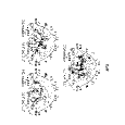
Figure 5: Galaxy distribution in the CfA2N catalogue projected onto three declination intervals.

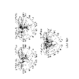
Figure 8: The CfALF catalogue corresponding to the SALF catalogue shown in Fig. 7 extracted from the $\Lambda$CDM simulation box.

Figs. 5, 6 and 7 show the CfA2N catalogue and two typical SALF catalogues from the $\tau$CDM and the $\Lambda$CDM simulations respectively. The $\tau$CDM mock catalogue does not look very much like the real Universe. There is too much structure within 5000 km s^-1 and the model fails to produce coherent sheets or filaments. These features are common to all our $\tau$CDM mock catalogues. The $\Lambda$CDM catalogues are in better qualitative agreement with the data. There are large voids and filaments extending across the full survey volume. Nevertheless, the structures are not as striking or as sharply defined as in the CfA2N. In addition, there is no structure comparable to the “Great Wall”. We have searched the simulation boxes for coherent sheets of galaxies and have failed to find anything as large as the observed wall (see also Schmalzing (1999)). It is unclear if this is a result of the relatively small volume of our simulations (particularly $\tau$CDM) or reflects a significant problem for the cosmological models we have studied. CfALF mock redshift surveys are closer in appearance to the CfA2N because the change in luminosity function forces a distribution of galaxies in redshift closer to that observed (Figure 8). Despite this the qualitative differences in large scale structure between the three cases remain.

In the following sections, we analyse the CfA2N and mock catalogues extracted from the simulations using identical techniques. We have compiled an ensemble of ten mock catalogues for each simulation in order to assess the robustness of our results. Note, however, that since all ten are constructed from the same parent simulation, the scatter between statistics estimated from them will underestimate the true sampling variance.

4 GROUPS IN REDSHIFT SPACE

A major problem for the study of groups in the real Universe is in finding an objective algorithm to define them, given that only partial knowledge of the phase space coordinates is available in real galaxy catalogues. This algorithm should select groups which correspond as closely as possible to real 3D groups, at least in a statistical sense. In the eighties, two main algorithms were proposed: the hierarchical method (e.g. Materne (1978); Tully (1980), 1987) and the friends-of-friends algorithm (Huchra & Geller (1982); Nolthenius & White (1987)).

We identify groups in our mock catalogues with the friends-of-friends algorithm described by Ramella et al. (1997). The robustness of methods of this type has been studied by Nolthenius & White (1987), Moore et al. (1993), and Frederic (1995a). All of these studies used dark matter–only $N$-body simulations to study the relation between groups selected from mock observational catalogues and genuine virialized systems. Their results were very similar to those we find below – with careful parameter choices it is possible to arrange a fair correspondence between the two kinds of system and to ensure that the statistical properties of groups estimated from the “observational” catalogues are quite similar to those of the “real” systems.

Sect. 4.1 reviews the friends-of-friends algorithm. In Sect. 4.2, we investigate the dependence of the statistical properties of groups on the linking parameters. In Sect. 5 we compare our models with the CfA2N groups. We find that variations of the galaxy luminosity function do affect the absolute abundances of groups, but have very little effect on their median properties.

4.1 Method

The friends-of-friends algorithm is an approximate method for identifying systems which lie above a chosen number overdensity threshold. We know galaxy positions in redshift space rather than in real space. We therefore need to use two distinct linking lengths, $V_{0}$ and $D_{0}$, for the radial velocity coordinate and the coordinates projected onto the sky, respectively. When we know the galaxy luminosity function $\phi(M)$, $D_{0}$ defines the number overdensity threshold

$${\delta n\over n}={3\over 4\pi D_{0}^{3}}\left[\int_{-\infty}^{M_{\rm lim}}\phi(M)dM\right]^{-1}-1$$ (1)

where $M_{\rm lim}=m_{\rm lim}-25-5{\rm Log}(cz_{f}/H_{0})$ is the faintest observable absolute magnitude at the fiducial redshift $cz_{f}=1000$ km s^-1 within a redshift survey with apparent limiting magnitude $m_{\rm lim}$. Having chosen the threshold $\delta n/n$ and the linking length, $V_{0}$, we link each pair of galaxies which satisfies

$${cz_{i}+cz_{j}\over H_{0}}\sin\left(\theta_{ij}\over 2\right)\leq D_{0}R_{ij}$$ (2)

$$|cz_{i}-cz_{j}|\leq V_{0}R_{ij}$$ (3)

where $cz_{i}$ and $cz_{j}$ are the galaxy radial velocities, $\theta_{ij}$ is their angular separation and

$$R_{ij}=\left[\int_{-\infty}^{M_{\rm lim}}\phi(M)dM\over\int_{-\infty}^{M_{ij}}\phi(M)dM\right]^{1/3}$$ (4)

where $M_{ij}=m_{\rm lim}-25-5{\rm Log}[(cz_{i}+cz_{j})/2H_{0}]$. Note that the scaling law in eq. (4) has been questioned by many authors. Specifically, replacing the power $1/3$ with $1/2$ (see the argument in Nolthenius & White (1987); Magtesyan (1988); Gourgoulhon, Chamaraux & Fouqué (1992)) drastically reduces the correlation between redshift and velocity dispersion observed in the Huchra & Geller (1982) group catalogue. However, part of this correlation is related to a selection effect rather than to the grouping algorithm, because groups with low velocity dispersion usually have few bright galaxies and so can only be seen at low redshift. Here, we use eq. (4) for consistency with the Ramella et al. (1997) catalogue.

One of the goals of identifying groups in the real Universe is to estimate their number density as a function of properties such as luminosity or velocity dispersion. To compute the correct abundance of groups, we weight each according to its distance (Moore et al. (1993)). We consider groups with $N\geq 3$ members. We can thus identify a group only when its third-ranked galaxy has absolute magnitude $M_{j}\leq m_{\rm lim}-25-5{\rm Log}(\langle cz\rangle/H_{0})$, where $\langle cz\rangle$ is the mean redshift of the group. $M_{j}$ determines the radius $cz_{j}$ of the sphere within which we could have identified this group. This group contributes with weight $1/\Psi_{j}$ to the total abundance of groups, where

$$\Psi_{j}={\Omega\over 3}\left(cz_{j}\over H_{0}\right)^{3}\left[1-{3z_{j}\over 2}\left(1+{\Omega_{0}\over 2}\right)\right]$$ (5)

is the proper volume sampled by the group, to first order in $z_{j}$, $\Omega$ is the solid angle of the survey and $\Omega_{0}$ is the (unknown) cosmological density parameter. We consider groups with $\langle cz\rangle\leq 12000$ km s^-1; therefore the first order correction in the volume is 9% at the most, when $\Omega_{0}=1$.

Note that the simulation galaxy catalogues are complete to $M_{B}=-17.5+5{\rm Log}h$. This magnitude sets a minimum redshift $cz_{\rm min}$: groups closer than $cz_{\rm min}$ could contain galaxies fainter than $M_{B}$ in a real magnitude limited survey. Therefore, we consider only redshift space groups with $\langle cz\rangle\geq cz_{\rm min}$ both in the mock catalogues and in the CfA2N catalogue.

4.2 Linking Parameters, Interlopers, and Physical Properties

From the CfA2N catalogue, Ramella et al (1997) compiled a fiducial group catalogue with linking parameters $\delta n/n=80$, and $V_{0}=350$ km s^-1. Here, we show that in the simulations these linking parameters give groups in redshift space with similar velocity dispersions and luminosities to the 3D groups (Sect 2.3) but with substantially larger sizes. These linking parameters will then be adopted for the remainder of our analysis.

The accidental inclusion of interlopers is one of the major problems in identifying groups in redshift space. Even with full knowledge of the galaxy locations in the six-dimensional phase space, the concept of interloper is ill-defined because groups are not isolated. Here, we define interlopers as follows. Each 3D group contains only galaxies lying within the same dark halo. Each member of a redshift space group is associated with some dark halo, but such a group may contain galaxies belonging to different dark halos. We define the dark halo containing the greatest number of group members as the group halo. All members belonging to another halo are then interlopers, and we define the interloper fraction $f_{\rm int}$ as the ratio between the number of interlopers and the total number of true members plus interlopers. If all members belong to different dark matter halos, the group is spurious and we set $f_{\rm int}=1$, because the group halo is undetermined.

Fig. 9 shows the dependence of $f_{\rm int}$ on the values of the linking parameters $V_{0}$ and $\delta n/n$ for two SALF redshift surveys. All the CfALF and SALF mock catalogues we compiled yield similar results. Squares show the median of the distribution of $f_{\rm int}$; error bars show the first and third quartiles. The solid square refers to the fiducial catalogue $\delta n/n=80$, $V_{0}=350$ km s^-1. It is apparent that $f_{\rm int}$ reaches a minimum when $\delta n/n\gtrsim 80-100$ and $V_{0}$ is small. Note that this minimum value is quite large; more than a third of the assigned members of a typical group are interlopers. Fig. 9 also shows that a significant fraction of groups are spurious; for the preferred values of $\delta n/n$ this fraction is 20 to 30%. We find that $\sim 40\%$ of the triplets are spurious, whereas only $\sim 20\%$ of the groups with four or more members are spurious. This result agrees with the suggestion of Ramella et al. (1989) that the physical association of triplets should be considered uncertain.

Fig. 10 shows how the weighted quartiles of the harmonic radius $R_{h}$ and of the velocity dispersion $\sigma$ vary with the linking parameters which define our catalogues. By weighted quartiles we mean the 25, 50 and 75% points of the cumulative distribution when each group is assigned weight $1/\Psi_{j}$ (see equation 5); these should correspond approximately to the quartiles of a volume limited group sample. For comparison we also plot the quartiles of the corresponding distributions for 3D groups as listed in Table 2. These figures show that $R_{h}$ depends only weakly on $V_{0}$ and is a decreasing function of $\delta n/n$; for $\delta n/n\gtrsim 80$ it depends little on either linking parameter. On the other hand, $\sigma$ is a strong function of $V_{0}$ for all $\delta n/n$. This systematic behaviour has been noted in all previous investigations of grouping algorithms; see Trasarti-Battistoni (1998) for a recent discussion. While our fiducial choice, $V_{0}=350$ km s^-1, leads to a $\sigma$ distribution which is similar to that of the true 3D groups, taking $\delta n/n=80$ results in $R_{h}$ distributions which are biased high by about a factor of two.

This bias in group size is related to the rather high interloper fraction noted above. If interlopers are excluded when calculating group properties, then the remaining galaxies are, by definition, all members of the same halo and so give a measure of group size which is statistically similar to that found using full 3D information. We demonstrate this in Tables 3 and 4, which compare the weighted quartiles of the distributions in mock redshift surveys including and excluding interlopers with those of the 3D groups repeated from Table 2. Excluding interlopers has little effect on the velocity dispersions of the groups but brings their estimated sizes and mass-to-light ratios into much better agreement with those of the 3D groups. Unfortunately, of course, it is not possible to exclude interlopers from real redshift survey group catalogues in this fashion.

It is curious that in our models this interloper-induced overestimation of $R_{h}$ in redshift survey groups combines with the overestimation of true group mass by $M_{\rm vir}$ (see section 2.3) to almost exactly cancel out the factor of 2.5 difference between the true mass-to-light ratio of groups and the mean mass-to-light ratio of the Universe. As a result, as may be seen in Tables 3 and 4, estimates of $\Omega_{0}$ obtained by multiplying the (incorrect) mean estimated $M_{\rm vir}/L_{B}$ by the average luminosity density are fortuitously quite close to the true value. It is difficult to judge whether this interloper-bias conspiracy will also work in the real Universe. Some of the tests we carry out below suggest that there is no reason to expect that these two biases should always be of the same order.

5 COMPARISON WITH THE CfA2N GROUPS

In this section, we compare our groups with the CfA2N catalogue. The galaxy luminosity function is a fundamental ingredient in constructing mock catalogues and in the friends-of-friends algorithm, so we might expect properties of groups in our simulated redshift surveys to depend strongly on the adopted luminosity function. We show below that this is only partly the case. We investigate how the luminosity function affects group abundances (Sect. 5.2) and the dependence of group properties on the linking parameters (Sect. 5.1).

5.1 Linking Parameters

In this section we study how the median group velocity dispersion $\sigma$ depends on the linking parameters used to define groups, and we compare with the behaviour seen in the CfA2N survey. The harmonic radius $R_{h}$ and the total group luminosity $L_{\rm tot}$ are also directly measurable, but, as we have shown, the estimated value of $R_{h}$ is biased high by interloper contamination, while $L_{\rm tot}$ is insensitive to the linking parameters. On the other hand, the velocity dispersion $\sigma$ is not significantly biased by interloper contamination and is sensitive to the linking parameter $V_{0}$. Moreover, the median $\sigma$ is a direct measure of the dynamics of galaxies on small scales, which in turn depends on the underlying mass distribution.

The left panels of Fig. 11 show that the trend of $\sigma$ with $V_{0}$ is similar in all our simulated redshift surveys and appears to be independent both of cosmological model ($\Lambda$CDM or $\tau$CDM) and of the adopted luminosity function (SALF or CfALF). The velocity dispersions of the simulated groups are systematically larger than the observed values by an amount which varies from about 10% at low $V_{0}$ to about 50% at large $V_{0}$. This difference is seen in all ten simulated surveys of each model.

Let us define the grouped fraction $N_{\rm gal}/N_{\rm tot}$ as the number of galaxies in groups divided by the total number of galaxies in the catalogue. Nolthenius et al. (1997) suggest using the dependence of the pair ($N_{\rm gal}/N_{\rm tot}$, $\sigma$) on $V_{0}$ at fixed $\delta n/n$ as a diagnostic to discriminate between models. Differences in the small-scale dynamics can show up as a shifting of the tracks in the $N_{\rm gal}/N_{\rm tot}$ – $\sigma$ plane. The right panels of Fig. 11 show such tracks for the CfA2N survey and for our simulated redshift surveys. Clearly, the choice of the luminosity function affects $N_{\rm gal}/N_{\rm tot}$ strongly but in opposite directions for our two models; if the SALF is used, the $\tau$CDM catalogue is closer than $\Lambda$CDM to the CfA2N; with the CfALF, we obtain the opposite result. Our models yield a fraction of galaxies in groups systematically lower than the CfA2N sample. When $V_{0}=350$ km s^-1, the fraction of galaxies in groups can be from $\sim 7\%$ (CfALF $\Lambda$CDM) to $\sim 30\%$ (SALF $\Lambda$CDM) smaller than in the CfA2N sample. Note however that the CfA2N track is less than two standard deviations from the CfALF $\Lambda$CDM track.

5.2 Group Abundances

Figs. 12 and 13 show the abundance of groups as a function of harmonic radius and velocity dispersion derived from our various catalogues. The top panels show results for the semi-analytic luminosity function (SALF). The discrepancy with the observations is simply a reflection of the overestimate (underestimate) of the total luminosity density of the Universe by $\tau$CDM ($\Lambda$CDM) as compared with CfA2N. When we impose the CfA survey luminosity function (bottom panels), the simulation results are in much better agreement with the observations, especially for $\Lambda$CDM.

The change in luminosity function from SALF to CfALF has a strong effect on the normalisation of the group abundance function, but rather little effect on its shape. As a result, the median properties of groups do not depend very strongly on the luminosity function. Tables 5 and 6 list the weighted quartiles of galaxy properties in the SALF and CfALF catalogues and compare them with the CfA2N values. Taking the variations between different mock catalogues into account, the median size and velocity dispersion of groups in the $\Lambda$CDM simulation agree reasonably well with the observations, if the CfALF is adopted. Moreover, we note that, according to our prescription for identifying galaxies in the simulations, the velocity of the central galaxy coincides with that of the dark matter particle with the greatest absolute value of the gravitational potential energy. This particle can move rapidly whereas the central galaxy is plausibly almost at rest with respect to the barycentre of its dark halo. When we replace the central galaxy velocity with the mean velocity of the dark particles within $r_{200}$, the median velocity dispersion of groups becomes $\sim 10\%$ smaller. This effect is sufficient to bring the CfALF $\Lambda$CDM model in good agreement with the CfA2N. On the other hand, groups in the $\tau$CDM simulation still have velocity dispersions slightly higher than observed.

Note that, on average, the difference between the central galaxy velocity and the barycentric velocity of its dark halo is $\sim 80$ km s^-1. Replacing the central galaxy velocity by the barycentric motion has a measurable effect on group dispersions because most groups are triplets and quadruplets. The same replacement does not affect the galaxy pairwise velocity statistics computed in section 6.

For both $\tau$CDM and $\Lambda$CDM, groups are significantly less luminous than in the real Universe. This is a consequence of the presence of the “Great Wall” in the CfA2N region: most of the groups lie within this structure at $\sim 7000-10000$ km s^-1 and so have a median redshift $\sim 8000$ km s^-1. In the models, however, the median group redshift is $\sim 6000$ km s^-1, leading to a typical luminosity a factor $\sim 2$ below that found for the CfA2N.

Note also that although for the SALF catalogues the interloper-bias conspiracy results in estimates of $\Omega_{0}$ which are quite close to the true values, the same conspiracy does not hold for the CfALF. Indeed, when our two simulations are forced to have the same luminosity function they produce group catalogues which are very similar in most of their properties. In particular, they have similar estimated mass-to-light ratios and so lead to similar estimates of $\Omega_{0}$ despite the factor of 3 difference between the true density values.

6 CORRELATION FUNCTIONS

To probe dynamics of galaxies on nonlinear scales, knowledge of galaxy peculiar velocities is necessary. Even for nearby galaxies direct measurements have $\sim 20$% uncertainties and only a relatively small number of measurements are currently available (see e.g. Strauss & Willick (1995) and references therein). Alternatively, we can study peculiar velocities statistically by using galaxy-galaxy redshift space correlation functions. Marzke et al. (1995) compute such correlation functions for the CfA redshift surveys. Here, we analyse our mock catalogues following their procedures which we summarise in the next section.

6.1 Method

In redshift space, the vector ${\bf s}_{i}=cz_{i}{\bf r}_{i}$ locates a galaxy with redshift $cz_{i}\ll c$ and celestial coordinates ${\bf r}_{i}=(\alpha_{i},\delta_{i})$. For small angular separations ($<50^{\rm o}$ in our analysis), we define the components of the relative separation ${\bf s}={\bf s}_{i}-{\bf s}_{j}$ of a pair of galaxies

$$\pi={{\bf s}\cdot{\bf l}\over|{\bf l}|},\quad r_{p}^{2}=s^{2}-\pi^{2}$$ (6)

where ${\bf l}=({\bf s}_{i}+{\bf s}_{j})/2$. The two-dimensional redshift space correlation function $\xi(r_{p},\pi)$ measures the excess probability, compared to a Poisson distribution, that a galaxy pair has separation $(r_{p},\pi)$. We estimate $\xi(r_{p},\pi)$ by weighting each galaxy according to the minimum variance estimator (Davis & Huchra (1982)).

By inverting $w(r_{p})$, the projection of $\xi(r_{p},\pi)$ onto the $r_{p}$ axis, we can estimate the spatial correlation function $\xi(r)$. Assuming a power-law, $w(r_{p})=Ar_{p}^{1-\gamma}$, gives $\xi(r)=(r/r_{0})^{-\gamma}$, and $A=r_{0}^{\gamma}\Gamma(1/2)\Gamma[(\gamma-1)/2]/\Gamma(\gamma/2)$.

On non-linear scales, we can then model $\xi(r_{p},\pi)$ as (e.g. Fisher (1995))

$$1+\xi(r_{p},\pi)=\int_{-\infty}^{\infty}\{1+\xi[(r_{p}^{2}+y^{2})^{1/2}]\}f(r_{p},\pi,y)dy$$ (7)

where the pairwise velocity distribution $f(r_{p},\pi,y)$ is well approximated by the exponential form

$$f(r_{p},\pi,y)=C(\sigma_{12})\exp\left[-{\sqrt{2}\over\sigma_{12}}\left|\pi-y-{y\over r}\langle v_{12}(r)\rangle\right|\right]$$ (8)

where $r^{2}=r_{p}^{2}+y^{2}$, and $y$ is the pair separation in real space along the line of sight. We model the mean streaming velocity $\langle v_{12}(r)\rangle$ with the scale-invariant solution to the truncated BBGKY hierarchy derived by Davis & Peebles (1983),

$$\langle v_{12}(r)\rangle=-{Fr\over 1+(r/r_{0})^{2}},$$ (9)

where the constant $F=1$ in the similarity solution.

Eq. (8) is an excellent approximation to the real distribution on very non-linear scales as already discussed by Sheth (1996) and Diaferio & Geller (1996). Eq. (8) also describes both dark matter particles and galaxies in our models quite accurately (Diaferio et al. (1999)). On mildly non-linear scales, infall skews the distributions. This skewness can be elegantly formalized with an Eulerian perturbative approach (Juszkiewicz, Fisher & Szapudi (1998)).

On the contrary, Eq. (9) is not a good approximation to the mean streaming velocity measured in the simulations. In Sect. 6.2 we will see that the uncertainty on $\langle v_{12}(r)\rangle$ does not strongly affect the estimate of the pairwise velocity dispersion $\sigma_{12}$, provided it is not assumed to be zero on all scales.

In order to estimate the pairwise velocity dispersion $\sigma_{12}(r_{p})$ at fixed projected separation $r_{p}$, we first determine the spatial correlation function $\xi(r)$; we then perform the integral in equation (7) by assuming $\sigma_{12}$ constant. Note, however, that $\sigma_{12}$ does depend on $y=(r^{2}-r_{p}^{2})^{1/2}$ because the cosmic virial theorem predicts $\sigma_{12}\propto r^{2-\gamma}$. However, since $\gamma\approx 2$, this procedure yields values of $\sigma_{12}$ in reasonable agreement with those computed with the full three-dimensional information. Finally, we use the measured $\xi(r_{p},\pi)$ to impose the normalisation $C(\sigma_{12})$ in equation (8). This procedure decreases the number of degrees of freedom by one.

To estimate errors on $\xi(r_{p},\pi)$ we use a bootstrap procedure with 50 resampled samples. Estimates of $\xi(r_{p},\pi)$ at different separations are correlated. Therefore, determining $\sigma_{12}$ by minimizing the $\chi^{2}$ computed directly with eq. (7) is not the correct procedure. Principal component analysis (Kendall (1975), Fisher et al. 1994a ) transforms a set of correlated quantities $\{\xi\}$ into a set of uncorrelated quantities $\{x\}$. Meaningful results come from the standard $\chi^{2}$ analysis applied to this latter set. Note that the errors of both the original and the transformed data sets are not Gaussian distributed. Therefore, the confidence levels of the computed $\chi^{2}$ should be considered only indicative.

6.2 Results

Fig. 14 shows the $\xi(r_{p},\pi)$ maps of our SALF and CfALF catalogues. At $r_{p}\lesssim 5h^{-1}$ Mpc, $\xi(r_{p},\pi)$ in the SALF $\tau$CDM catalogue is larger than in the CfALF catalogue; the SALF catalogue contains more galaxies in groups and clusters. On the other hand the two $\xi(r_{p},\pi)$ maps for the $\Lambda$CDM model are very similar, perhaps because the differences between the two luminosity functions are smaller.

We can quantify the differing behaviour of our two models by looking at the parameters $r_{0}$ and $\gamma$ of the real space correlation function derived by fitting a power law to the projected correlation function $w(r_{p})$. Table 7 shows that $r_{0}$ decreases by $35\%$ from the SALF to the CfALF catalogue in the $\tau$CDM model, while in the $\Lambda$CDM model there is no significant change. None of these models matches the CfA2N parameters satisfactorily, perhaps because the CfA2N yields a correlation length which is significantly larger than in other surveys: CfA2 South and SSRS2 have $r_{0}=4.75$ and $5.08h^{-1}$ Mpc respectively (Marzke et al. (1995)), while the LCRS gives $5.06h^{-1}$ Mpc (Jing et al. (1998)); these values are close to those of our models. Note that CfA2 South also has $\gamma=1.99$, so that its correlation function is in close agreement with that of our $\Lambda$CDM model.

We find a similar result by looking at the projection of $\xi(r_{p},\pi)$ onto the $\pi$ axis averaged over the $r_{p}$ interval $(r_{p}^{1},r_{p}^{2})$

$$\langle\xi(\pi)\rangle={1\over r_{p}^{2}-r_{p}^{1}}\int_{r_{p}^{1}}^{r_{p}^{2}}\xi(r_{p},\pi)dr_{p}$$ (10)

(Figs. 15 and 16). Independently of the luminosity function, both models predict a correlation amplitude somewhat smaller than that of the CfA2N. Typical amplitude ratios between the CfA2N and the models are in the range $\sim 1.0-2.3$. These differences are similar to those between the CfA2N and CfA2 South or SSRS2 (Marzke et al. (1995)).

Small variations in $\langle\xi(\pi)\rangle$ translate into large variations in the best fit parameters $\sigma_{12}$. In fact, Marzke et al. (1995) show that $\sigma_{12}$ can vary by a factor as large as three from survey to survey. In Fig. 17, solid squares show $\sigma_{12}(r_{p})$ when the similarity solution for the mean streaming velocity is assumed ($F=1$ in eq. [9]). The bold solid line is the $\sigma_{12}$ of galaxies computed with the full three-dimensional information. The variations in the amplitude and slope of $\langle\xi(\pi)\rangle$ between SALF and CfALF catalogues make $\sigma_{12}$ vary by $\sim 200$ km s^-1. However, given the sensitivity of $\sigma_{12}$, the differences between the models are not significant: both models predict a $\sigma_{12}(r_{p})$ profile close to that of the CfA2N, independently of the luminosity function adopted. A more robust statistic, e.g. the single-particle-weighted statistic $\sigma_{1}$ suggested by Davis, Miller & White (1997), might provide a more convincing comparison.

Finally, we note that in our models $\langle v_{12}(r)\rangle$ is significantly different from zero at megaparsec scales; moreover, the similarity solution (eq. [9]) does not describe its behaviour adequately. However, the estimated $\sigma_{12}$ are only weakly dependent on the form of $\langle v_{12}(r)\rangle$. For comparison, we estimate $\sigma_{12}$ with $F=2.5$ and $r_{0}=3h^{-1}$ Mpc which appears to be a better fit to $\langle v_{12}(r)\rangle$ in our simulations. The agreement between the estimated $\sigma_{12}(r_{p})$ and the three-dimensional profile does not improve substantially (open triangles in the top panels of Fig. 17). On the other hand, in agreement with the result of Marzke et al. (1995), assuming $F=0$ underestimates $\sigma_{12}(r_{p})$ significantly (open squares in Fig. 17). This raises a serious question about the Fourier method suggested by Landy, Szalay & Broadhurst (1998) for estimating $\sigma_{12}(r_{p})$: this method necessarily assumes $\langle v_{12}(r)\rangle=0$.

7 CONCLUSION

In Paper I, we simulated the formation, evolution and clustering of galaxies by combining dissipationless $N$-body simulations and semi-analytic models of galaxy formation. We investigated a high density universe ($\tau$CDM) and a low density universe with a cosmological constant ($\Lambda$CDM). Here, we extract wide angle mock redshift surveys from these simulations and compare them with the CfA2N redshift survey by compiling catalogues of galaxy groups and by computing the redshift space correlation function $\xi(r_{p},\pi)$.

Despite their very different $\Omega_{0}$ values, both models yield a reasonable match to the data, although both appear slightly less clustered than the CfA2N: for example, $\sim 30\%$ ($\tau$CDM) and $\sim 23\%$ ($\Lambda$CDM) of galaxies are in groups rather than the $32\%$ observed; moreover, the amplitude of $\xi(r_{p},\pi)$ is systematically a factor $\sim 1.5-2.0$ smaller than observed. However, this weaker clustering is similar to that observed in the southern regions of the CfA redshift surveys and in the LCRS, suggesting that galaxies within the CfA2N catalogue might be unusually highly clustered.

Our semi-analytic modelling predicts luminosity functions which fit the CfA results rather poorly. To test whether this disagreement induces clustering differences between our mock surveys and the CfA2N galaxy catalogue, we impose the CfA survey luminosity function on the models. We find that in fact only the group abundances are strongly affected, becoming substantially closer to those observed in the modified catalogues. Quantities connected with the underlying mass distribution, such as the median velocity dispersion of groups or the redshift space correlation function, show less sensitivity to the adopted luminosity function.

We compare our models with the CfA2N because (1) this survey provides the largest catalogue of galaxy groups currently available, and (2) it covers a volume similar to that we have simulated. However, a coherent two-dimensional structure, the “Great Wall”, dominates the large scale distribution of galaxies in the CfA2N and is not reproduced in our simulations. This structure plays a significant role in determining the typical luminosities of the observed groups and may also affect other group properties. It is unclear whether the apparent deficiency of coherent two-dimensional structure in our mock catalogues is a significant problem for our cosmological models, or reflects cosmic variance and the relatively small size of our simulation boxes. The modest discrepancies between our models and the CfA2N could plausibly disappear when other surveys, covering larger volumes and based on better photometric data become available, and can be compared with simulations of similarly large cosmological volumes.

Given the limitations of the observational and numerical data we consider in this paper, the agreement between theory and observation is remarkable and demonstrates that present day group dynamics alone give little information about $\Omega_{0}$. Our preference for $\Lambda$CDM over $\tau$CDM is based on its better agreement with the observed luminosity functions and Tully-Fisher relations (Paper I) and with the observed evolution of clustering (Paper II) rather than on any difference in pairwise velocities or in the mass-to-light values implied for groups. On the other hand, these clustering differences reflect observable differences in the evolution of groups and clusters and of their galaxy populations which should be detectable in future surveys to higher redshift. We will investigate these issues more thoroughly in a forthcoming paper.

Appendix A APPENDIX

For reference, we review here the formulae we use to compute the physical properties of groups.

A system with $N$ galaxies has three-dimensional (3D) harmonic radius

$$R_{h}={N(N-1)\over 2}\left(\sum_{i=1}^{N-1}\sum_{j=i+1}^{N}{1\over|{\bf r}_{ij}|}\right)^{-1}$$ (A1)

where ${\bf r}_{ij}$ are the pairwise galaxy separations. The corresponding harmonic radius for a real system at redshift $\langle cz\rangle$ is

$$R_{h}={\pi\over 2}{\langle cz\rangle\over H_{0}}N(N-1)\left[\sum_{i=1}^{N-1}\sum_{j=i+1}^{N}{1\over\tan(\theta_{ij}/2)}\right]^{-1}$$ (A2)

where $\theta_{ij}$ are the pairwise galaxy angular separations and $H_{0}$ is the Hubble constant.

The one-dimensional velocity dispersion from the 3D velocities is

$$\sigma=\left[{1\over 3(N-1)}\sum_{i=1}^{N}({\bf v}_{i}-\langle{\bf v}\rangle)^{2}\right]^{1/2},$$ (A3)

whereas from the line-of-sight velocities it is

$$\sigma=\left[{1\over N-1}\sum_{i=1}^{N}(cz_{i}-\langle cz\rangle)^{2}\right]^{1/2}.$$ (A4)

The combination of $R_{h}$ and $\sigma$ provides the virial mass via the virial theorem

$$M_{\rm vir}={6\sigma^{2}R_{h}\over G}$$ (A5)

where $G$ is the gravitational constant.

The total luminosity of a galaxy group is the sum of the contribution from the $N$ galaxies observed and the contribution from galaxies which are too faint to be observed:

$$L_{\rm tot}=L_{\rm faint}+\sum_{i=1}^{N}L_{i}.$$ (A6)

We can estimate the contribution of the faint galaxies by assuming the luminosity function to be universal:

$$L_{\rm faint}={\rm Volume}\times\langle L_{\rm faint}\rangle={N\over\int_{L_{\rm lim}}^{\infty}\phi(L)dL}\times\int_{0}^{L_{\rm lim}}L\phi(L)dL$$ (A7)

where $L_{\rm lim}$ is the luminosity of the faintest observable galaxy within the group. We adopt the usual Schechter form of the luminosity function

$$\phi(L)dL=\phi^{*}(L/L^{*})^{\alpha}\exp(-L/L^{*})d(L/L^{*})$$ (A8)

or equivalently

$$\phi(M)dM=0.4\ln 10\phi^{*}10^{-0.4(M-M^{*})(\alpha+1)}\exp[-10^{-0.4(M-M^{*})}]dM$$ (A9)

when absolute magnitudes $M$ are used.

Table 1: Luminosity Function Parameters

	$\alpha$	$M_{B}^{*}-5{\rm Log}h$	$\phi^{*}/{\rm gal}\ {\rm mag}^{-1}h^{3}{\rm Mpc}^{-3}$
$\tau$CDM	$-1.67\pm 0.01$	$-21.05\pm 0.03$	$(5.8\pm 1.0)\times 10^{-3}$
$\Lambda$CDM	$-1.40\pm 0.01$	$-20.13\pm 0.02$	$(4.1\pm 0.8)\times 10^{-3}$
CfA	$-1.00\pm 0.20$	$-18.80\pm 0.30$	$(4.0\pm 1.0)\times 10^{-2}$

Note. — Parameters and 1-$\sigma$ standard deviations of the Schechter function fit to the model luminosity functions (Fig. 1) and the CfA Redshift Survey (Marzke et al. (1994)).

Table 2: 3D Groups

	$\tau$CDM	$\Lambda$CDM
$N_{\rm gal}/N_{\rm tot}$	0.30	0.25
$R_{h}$	0.13/0.21/0.29	0.15/0.27/0.43
$\sigma$	149/213/296	179/246/335
${\rm Log}M_{\rm vir}$	12.69/13.05/13.47	12.92/13.30/13.69
$M_{\rm vir}/M_{200}$	0.88/1.37/2.04	0.76/1.33/2.13
${\rm Log}L_{B}$	10.53/10.66/10.89	10.48/10.61/10.83
${\rm Log}(M_{\rm vir}/L_{B})$	2.09/2.37/2.61	2.39/2.67/2.93
$\Omega_{0}^{\rm est}$	0.55	0.18

Note. — Quartiles of the distributions for the galaxy groups within the box. $R_{h}$, $\sigma$, $M_{\rm vir}$, $L_{B}$, and $M_{\rm vir}/L_{B}$ are in units of $h^{-1}$ Mpc, km s^-1, $h^{-1}M_{\odot}$, $h^{-2}L_{\odot}$, and $hM_{\odot}/L_{\odot}$, respectively. $M_{200}$ is the dark halo mass within $r_{200}$.

Table 3: Redshift Space Groups: $\tau$CDM

	RS	RSc	3D
$N_{\rm gal}/N_{\rm tot}$	0.30	0.20	0.30
$R_{h}$	0.22/0.35/0.55	0.15/0.25/0.32	0.13/0.21/0.29
$\sigma$	121/216/336	151/227/378	149/213/296
${\rm Log}M_{\rm vir}$	12.87/13.25/13.79	12.73/13.15/13.80	12.69/13.05/13.47
${\rm Log}L_{B}$	10.51/10.69/10.93	10.61/10.77/10.99	10.53/10.66/10.89
${\rm Log}(M_{\rm vir}/L_{B})$	2.14/2.49/2.95	1.92/2.36/2.71	2.09/2.37/2.61
$\Omega_{0}^{\rm est}$	0.72	0.54	0.55

Note. — Weighted quartiles of the distributions for the galaxy group catalogue from the $\tau$CDM SALF survey shown in Fig. 6: RS refers to groups identified in redshift space, RS_c to groups identified in redshift space with interlopers excluded, and 3D to properties derived from the 3D galaxy distribution. Quantities are in the same units as in Table 2.

Table 4: Redshift Space Groups: $\Lambda$CDM

	RS	RSc	3D
$N_{\rm gal}/N_{\rm tot}$	0.23	0.15	0.25
$R_{h}$	0.35/0.59/0.80	0.18/0.34/0.55	0.15/0.27/0.43
$\sigma$	135/222/345	164/223/368	179/246/335
${\rm Log}M_{\rm vir}$	12.97/13.53/13.91	12.88/13.37/13.80	12.92/13.30/13.69
${\rm Log}L_{B}$	10.44/10.65/10.90	10.54/10.71/11.00	10.48/10.61/10.83
${\rm Log}(M_{\rm vir}/L_{B})$	2.37/2.82/3.22	2.28/2.64/3.00	2.39/2.67/2.93
$\Omega_{0}^{\rm est}$	0.25	0.17	0.18

Note. — Same as Table 3 for the $\Lambda$CDM SALF survey shown in Fig. 7.

Table 5: Luminosity Function Effect: $\tau$CDM

	SALF	CfALF	CfA2N
$N_{\rm gal}/N_{\rm tot}$	0.30	0.22	0.32
$R_{h}$	0.22/0.35/0.55	0.21/0.39/0.59	0.23/0.44/0.71
$\sigma$	121/216/336	134/225/336	99/183/299
${\rm Log}M_{\rm vir}$	12.87/13.25/13.79	12.80/13.39/13.82	12.60/13.19/13.84
${\rm Log}L_{B}$	10.51/10.69/10.93	10.34/10.52/10.79	10.52/10.88/11.19
${\rm Log}(M_{\rm vir}/L_{B})$	2.14/2.49/2.95	2.28/2.76/3.14	1.77/2.43/2.84
$\Omega_{0}^{\rm est}$	0.72	0.43	0.20

Note. — Weighted quartiles of the distributions for the redshift space group catalogues from two corresponding $\tau$CDM surveys differing in the luminosity function adopted. The SALF survey is shown in Fig. 6. CfA2N column is for the groups in the CfA2N catalogue. Quantities are in the same units as in Table 2.

Table 6: Luminosity Function Effect: $\Lambda$CDM

	SALF	CfALF	CfA2N
$N_{\rm gal}/N_{\rm tot}$	0.23	0.30	0.32
$R_{h}$	0.35/0.59/0.80	0.31/0.46/0.64	0.23/0.44/0.71
$\sigma$	135/222/345	122/207/305	99/183/299
${\rm Log}M_{\rm vir}$	12.97/13.53/13.91	12.87/13.38/13.77	12.60/13.19/13.84
${\rm Log}L_{B}$	10.44/10.65/10.90	10.45/10.65/10.87	10.52/10.88/11.19
${\rm Log}(M_{\rm vir}/L_{B})$	2.37/2.82/3.22	2.27/2.69/3.10	1.77/2.43/2.84
$\Omega_{0}^{\rm est}$	0.25	0.37	0.20

Note. — Same as Table 5 for two $\Lambda$CDM surveys. The SALF survey is shown in Fig. 7.

Table 7: Correlation Function $\xi(r)$

	$r_{0}/h^{-1}$ Mpc	$\gamma$	$\chi_{18}^{2}$
$\tau$CDM SALF	$5.00\pm 0.13$	$1.69\pm 0.03$	0.69
$\tau$CDM CfALF	$3.20\pm 0.28$	$1.95\pm 0.11$	0.51
$\Lambda$CDM SALF	$4.45\pm 0.11$	$2.03\pm 0.03$	1.24
$\Lambda$CDM CfALF	$4.33\pm 0.22$	$2.02\pm 0.07$	1.24
CfA2N	$5.59\pm 0.24$	$1.82\pm 0.04$	0.63

Note. — Parameters of the correlation function fits for individual mock catalogues. The SALF catalogues are shown in Figs. 6 and 7. The scatter between values from different mock catalogues is about $5\%$.

Figure 1: Upper panels: Blue band galaxy luminosity function for our models. Error bars are Poisson 1-$\sigma$ standard deviations. Solid, long-dashed, dot-dashed, and dotted lines are the CfA (Marzke et al. (1994)), LCRS (Lin et al. (1996)), Stromlo-APM (Loveday et al. (1992)), and ESP (Zucca et al. (1997)) luminosity functions, respectively. Lower panels: Luminosity function of galaxies within halos of different mass: long-dashed line, $M_{200}>10^{14}h^{-1}M_{\odot}$; short-dashed line, $10^{13}h^{-1}M_{\odot}<M_{200}\leq 10^{14}h^{-1}M_{\odot}$; dotted line, $10^{12}h^{-1}M_{\odot}<M_{200}\leq 10^{13}h^{-1}M_{\odot}$; thin solid line, $M_{200}\leq 10^{12}h^{-1}M_{\odot}$. The bold solid line is the total luminosity function.

Figure 2: Average number overdensity profiles $\langle\delta(<r)\rangle$ and bias $b$ of galaxies relative to dark matter in halos with mass $M_{200}>10^{14}h^{-1}M_{\odot}$. Central galaxies of each halo are excluded in the computation of the profiles. The two left most (right most) columns are for the $\tau$CDM ($\Lambda$CDM) model. First and third column: solid, dot-dashed, and long-dashed lines are for dark matter and galaxies brighter than $M_{B}-5{\rm Log}h=-17.5$, and $-19.5$, respectively. Second and fourth column: solid and dot-dashed (short-dashed) lines are for dark matter and galaxies brighter than $M_{B}=-17.5+5{\rm Log}h$ and with colour $B-I\leq 1.75$ ($B-I>1.75$), respectively. The colour cut is at the median of the colour distribution which is the same for both cosmologies.

Figure 3: Surface number density profiles of galaxies within halos with mass $M_{200}>10^{14}h^{-1}M_{\odot}$ compared with observed cluster samples as explained in the text. Solid (dashed) lines show the profiles for red (blue) galaxies in the models. Crosses and triangles are for red and blue galaxies in the CNOC sample (left panels) and for non-emission-line galaxies and emission-line galaxies for the ENACS sample (right panels). The fraction of galaxies in each subsample is the same for both models and observations.

Figure 4: Velocity dispersion profiles in units of the circular velocity $V_{200}$ and velocity bias of galaxies relative to the dark matter. Panels and lines are as in Fig. 2.

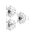
Figure 6: Same as Fig. 5 for a SALF catalogue extracted from the $\tau$CDM simulation box.

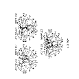
Figure 7: Same as Fig. 5 for a SALF catalogue extracted from the $\Lambda$CDM simulation box.

Figure 9: Upper panels: Median of the fraction of interlopers $f_{\rm int}$ within an individual group in group catalogues extracted from the two SALF catalogues shown in Figs. 6 and 7 with different linking parameters $\delta n/n$ and $V_{0}$. Squares are the weighted medians of the distributions, error bars show the lower and upper quartiles. At fixed $\delta n/n$, quantities for $V_{0}=150$, 350, and 550 km s^-1 are shown; quantities for $V_{0}>150$ km s^-1 are shifted to the right for clarity. Solid square refers to the fiducial catalogue. Lower panels: Fraction $f_{\rm sp}$ of spurious groups.

Figure 10: Dependence of the group median properties on the linking parameters $\delta n/n$ and $V_{0}$ in the SALF catalogues of Figs. 6 and 7. Values of $V_{0}$ are as in Fig. 9. Error bars show the upper and lower quartiles. Solid lines show the quartiles of the 3D group catalogue.

Figure 11: Left Panels: Weighted median velocity dispersion $\sigma$ of group catalogues versus the linking parameter $V_{0}$ at fixed $\delta n/n=80$. Triangles, open and solid squares indicate the CfA2N, $\tau$CDM and $\Lambda$CDM catalogues respectively. Model groups are extracted from the galaxy catalogues with the semi-analytic model luminosity function (top panel) or the imposed CfA luminosity function (bottom panel). Points show the mean values averaged over the ensamble of ten mock catalogues. Error bars are the 1-$\sigma$ standard deviations. Solid squares ($\Lambda$CDM model) are slightly shifted to the left for clarity. Right Panels: $\sigma$ versus the fraction of galaxies in groups $N_{\rm gal}/N_{\rm tot}$ for the same catalogues of the left panels. Points from left to right correspond to increasing $V_{0}$. Symbols are as for the left panels.

Figure 12: Group abundance by harmonic radius $R_{h}$. Number densities are estimated for catalogues extracted with $\delta n/n=80$ and $V_{0}=350$ km s^-1. Bold lines are the mean number densities averaged over the ensamble of ten mock catalogues. Shaded areas show the 3-$\sigma$ deviations. Dashed lines are for the CfA2N groups. Error bars on the CfA2N curves are Poisson 3-$\sigma$ deviations.

Figure 13: Group abundance by velocity dispersion $\sigma$. Lines and deviations are as in Fig. 12.

Figure 14: Maps of the two dimensional correlation function $\xi(r_{p},\pi)$. Top panels are for the SALF catalogues of Figs. 6 and 7. Bottom panels are for the corresponding CfALF catalogues. The bold contour indicates $\xi(r_{p},\pi)=1$. Contour levels are separated by logarithmic intervals of 0.1 for $\xi(r_{p},\pi)>1$ and by linear intervals of 0.1 for $\xi(r_{p},\pi)<1$. Dashed contours indicate $\xi(r_{p},\pi)<0$.

Figure 15: Correlation functions projected onto the $\pi$ axis for different intervals of the projected separation $r_{p}$ for the SALF $\tau$CDM catalogue shown in Fig. 6 (squares). Intervals of $r_{p}$ in units of $h^{-1}$ Mpc are shown in the right upper corner of each panel. Bold solid lines show the best fits to eq. (10). Thin solid lines are the best fits for the corresponding CfALF catalogue. Long dashed lines are the best fits for the CfA2N catalogue. All curves are for $F=1$ in eq. (9). $\langle\xi(\pi)\rangle$ curves for the ten mock catalogues can differ by $\sim 10-20\%$ depending on the $r_{p}$ interval.

Figure 16: Same as Fig. 15 for the $\Lambda$CDM catalogue of Fig. 7.

Figure 17: Pairwise velocity dispersion $\sigma_{12}$ at different projected separations $r_{p}$ corresponding to the curves in Figs. 15 and 16. Solid (open) squares are for $F=1$ ($F=0$) in eq. (9). In the top panels, triangles are for $F=2.5$ and $r_{0}=3h^{-1}$ Mpc in eq. (9). The $\sigma_{12}(r_{p})$ profiles have a scatter of $\sim 15\%$ for different mock catalogues. Bold lines show the three-dimensional pairwise velocity dispersion of galaxies brighter than $M_{B}=-17.5+5{\rm Log}h$ (Paper I); the dashed line is the CfA2N profile when $F=1$ (Marzke et al. (1995)).

References

- Allen (1973) Allen, C. W. 1973, Astrophysical Quantities, 3rd edition, Athlone Press, London
- Baugh, Cole & Frenk (1996) Baugh, C. M., Cole, S., & Frenk, C. S. 1996, MNRAS, 283, 1361
- Biviano et al. (1995) Biviano, A., et al. 1995, A&A, 297, 610
- Biviano et al. (1997) Biviano, A., Katgert, P., Mazure, A., Moles, M., den Hartog, R., Perea, J., & Focardi, P. 1997, A&A, 321, 84
- Biviano et al. (1998) Biviano, A., Mazure, A., Adami, C., Katgert, P., den Hartog, R., de Theije, P. A. M., & Rhee, G. 1998, in Observational Cosmology: The Developments of Galaxy Systems, astro-ph/9810501
- Blanton et al. (1998) Blanton, M., Cen, R., Ostriker, J. P., & Strauss, M. A. 1998, ApJ, submitted (astro-ph/9807029)
- Bond et al. (1991) Bond, J. R., Cole, S., Efstathiou, G., & Kaiser, N. 1991, ApJ, 379, 440
- Bower (1991) Bower, R. J. 1991, MNRAS, 248, 332
- Carlberg (1991) Carlberg, R. G. 1991, ApJ, 367, 385
- Carlberg et al. (1996) Carlberg, R. G., Yee, H. K. C., Ellingson, E., Abraham, R., Gravel, P., Morris, S., & Pritchet, C.J. 1996, ApJ, 462, 32
- Carlberg et al. (1997) Carlberg, R. G., et al. 1997, ApJ, 476, L7
- Cen & Ostriker (1998) Cen, R., & Ostriker, J. P. 1998, ApJ, submitted (astro-ph/9809370)
- Cole et al. (1994) Cole, S., Aragón-Salamanca, A., Frenk, C. S., Navarro, J. F., & Zepf, S. E. 1994, MNRAS, 271, 781
- Cole et al. (1998) Cole, S., Hatton, S., Weinberg, D. H., & Frenk, C. S. 1998, MNRAS, 300, 945
- Couchman & Carlberg (1992) Couchman, H. M. P., & Carlberg, R. G. 1992, ApJ, 389, 453
- Davis, Mulchaey & Mushotzky (1998) Davis, D. S., Mulchaey, J. S., & Mushotzky, R. F. 1998, astro-ph/9808085
- Davis & Huchra (1982) Davis, M., & Huchra, J. P. 1982, ApJ, 254, 437
- Davis & Peebles (1983) Davis, M., & Peebles, P. J. E. 1983, ApJ, 267, 465
- Davis et al. (1985) Davis, M., Efstathiou, G., Frenk, C. S., & White, S. D. M. 1985, ApJ, 292, 371
- Davis, Miller & White (1997) Davis, M., Miller, A., & White, S. D. M. 1997, ApJ, 490, 63
- de Lapparent, Geller & Huchra (1991) de Lapparent, V., Geller, M. J., & Huchra, J. P. 1991, ApJ, 369, 273
- de Theije & Katgert (1998) de Theije, P. A. M., & Katgert, P. 1998, A&A, in press (astro-ph/9811199)
- Diaferio & Geller (1996) Diaferio, A., & Geller, M. J. 1996, ApJ, 467, 19
- Diaferio et al. (1993) Diaferio, A., Ramella, M., Geller, M. J., & Ferrari, A. 1993, AJ, 105, 2035
- Diaferio et al. (1999) Diaferio, A., Kauffmann, G., Colberg, J. M., & White, S. D. M. 1999, in The Birth of Galaxies, Proceedings of the X Rencontres de Blois, ed. B. Guiderdoni, in press
- Dressler (1980) Dressler, A. 1980, ApJ, 236, 351
- Dressler et al. (1997) Dressler, A., et al. 1997, ApJ, 490, 577
- Ferrerira et al. (1999) Ferrerira, P. G., Juszkiewicz, R., Feldman, H. A., Davis, M., & Jaffe, A. H., 1999, astro-ph/9812456
- Fisher (1995) Fisher, K. B. 1995, ApJ, 448, 494
- (30) Fisher, K. B., Davis, M., Strauss, M. A., Yahil, A., & Huchra, J. P. 1994a, MNRAS, 266, 50
- (31) Fisher, K. B., Davis, M., Strauss, M. A., Yahil, A., & Huchra, J. P. 1994b, MNRAS, 267, 927
- Frederic (1995a) Frederic, J. J. 1995a, ApJS, 97, 259
- (33) Frederic, J. J. 1995b, ApJS, 97, 275
- Gelb & Bertschinger (1994) Gelb, J. M., & Bertschinger, E. 1994, ApJ, 436, 491
- Geller & Huchra (1983) Geller, M. J., & Huchra, J. P. 1983, ApJS, 52, 61
- Geller & Huchra (1989) Geller, M. J., & Huchra, J. P. 1989, Science, 246, 897
- Gilmore, King & van der Kruit (1990) Gilmore, G. F., King, I. R., & van der Kruit, P. C. 1990, The Milky Way as a Galaxy, 19th Saas-Fee Advanced Course, Geneva, Switzerland
- Giovanelli et al. (1997) Giovanelli, R. M., Haynes, M. P., Da Costa, L. N., Freudling, W., Salzer, J. J., & Wegner, G. 1997, ApJ, 477, L1
- Giuricin et al. (1988) Giuricin, G. Gondolo, P., Mardirossian, F. Mezzetti, M., & Ramella, M. 1988, A&A, 199, 85
- Gourgoulhon, Chamaraux & Fouqué (1992) Gourgoulhon, E., Chamaraux, P., & Fouqué, P. 1992, A&A, 255, 69
- Gurzadyan & Mazure (1998) Gurzadyan, V. G., & Mazure, A. 1998, in Untangling Coma Berenices: A New Vision of an Old Cluster, ed. A. Mazure, F. Casoli, F. Durret, & D. Gerbal, (Singapore: Word Scientific), 54
- Hickson (1997) Hickson, P. 1997, ARA&A, 35, 357
- Huchra & Geller (1982) Huchra, J. P., & Geller, M. J. 1982, ApJ, 257, 423
- Huchra et al. (1990) Huchra, J. P., de Lapparent, V., Geller, M. J., & Corwin, Jr., H. G. 1990, ApJS, 72, 433
- Huchra, Geller & Corwin (1995) Huchra, J. P., Geller, M. J., & Corwin, Jr., H. G. 1995, ApJS, 99, 391
- Jenkins et al. (1998) Jenkins, A., Pearce, F., et al. 1998, in preparation
- Jing et al. (1998) Jing, Y. P., Mo, H. J., & Börner, G. 1998, ApJ, 494, 1
- Juszkiewicz, Fisher & Szapudi (1998) Juszkiewicz, R., Fisher, K. B., & Szapudi, I. 1998, ApJ, 504, L1
- Juszkiewicz, Springel & Durrer (1999) Juszkiewicz, R., Springel, V., & Durrer, R. 1999, ApJ, submitted
- Kauffmann & White (1993) Kauffmann, G., & White, S. D. M. 1993, MNRAS, 261, 921
- Kauffmann, White & Guiderdoni (1993) Kauffmann, G., White, S. D. M., & Guiderdoni, B. 1993, MNRAS, 264, 201
- (52) Kauffmann, G., Colberg, J. M., Diaferio, A., & White, S. D. M., 1999a, MNRAS, 303, 188 (Paper I)
- (53) Kauffmann, G., Colberg, J. M., Diaferio, A., & White, S. D. M., 1999b, MNRAS, in press (Paper II)
- Kendall (1975) Kendall, M. 1975, Multivariate Analysis, Charles Griffin & Co., London
- Kennicutt (1998) Kennicutt, R. C. 1998, ApJ, 498, 541
- Koranyi et al. (1998) Koranyi, D., Geller, M. J., Mohr, J. J., & Wegner, G. 1998, AJ, in press
- Lacey & Cole (1993) Lacey, C. G., & Cole, S. M. 1993, MNRAS, 262, 627
- Lacey & Silk (1991) Lacey, C., & Silk, J. 1991, ApJ, 381, 14
- Landy, Szalay & Broadhurst (1998) Landy, S. D., Szalay, A. S., & Broadhurst, T. J. 1998, ApJ, 494, L133
- Lin et al. (1996) Lin, H., Kirshner, R. P., Schectman, S. A., Landy, S. D., Oemler, A., Tucker, D. L., Schechter, P. L. 1996, ApJ, 464, 60
- Loveday et al. (1992) Loveday, J., Peterson, B. A., Efstathiou, G., Maddox, S. J. 1992, ApJ, 390, 338
- Magtesyan (1988) Magtesyan, A. P. 1988, Astrophysics, 28, 150
- Mahdavi et al. (1998) Mahdavi, A., Geller, M. J., et al. 1998, in preparation
- Mamon (1993) Mamon, G. A. 1993, in Gravitational Dynamics and the -body Problem, ed. F. Combes & E. Athanassoula (Paris: Observatoire de Paris), 188
- Marzke et al. (1994) Marzke, R. O., Huchra, J. P., & Geller, M. J. 1994, ApJ, 428, 43
- Marzke et al. (1995) Marzke, R. O., Geller, M. J., da Costa, L. N., & Huchra, J. P. 1995, AJ, 110, 477
- Materne (1978) Materne, J. 1978, A&A, 63, 401
- Mo et al. (1993) Mo, H. J., Jing, Y. P., & Börner, G. 1993, MNRAS, 264, 825
- Mohr et al. (1996) Mohr, J. J., Geller, M. J., Fabricant, D. G., Wegner, G., Thorstensen, J., & Richstone, D. O., 1996, ApJ, 470, 724
- Molinari et al. (1998) Molinari, E., Chincarini, G., Moretti, A., & de Grandi, S. 1998, A&A, 338, 874
- Moore et al. (1993) Moore, B., Frenk, C. S., & White, S. D. M. 1993, MNRAS, 261, 827
- Moss & Dickens (1977) Moss, C., & Dickens, R. J. 1977, MNRAS, 178, 701
- Mulchaey et al. (1996) Mulchaey, J. S., Davis, D. S., Mushotzky, R. F., & Burstein, D. 1996, ApJ, 456, 80
- Navarro, Frenk & White (1995) Navarro, J. F., Frenk, C. S., & White, S. D. M. 1995, MNRAS, 275, 56
- Navarro, Frenk & White (1997) Navarro, J. F., Frenk, C. S., & White, S. D. M. 1997, ApJ, 490, 493
- Nolthenius (1993) Nolthenius, R. A. 1993, ApJS, 85, 1
- Nolthenius & White (1987) Nolthenius, R. A., & White, S. D. M. 1987, MNRAS, 235, 505
- Nolthenius et al. (1997) Nolthenius, R. A., Klypin, A. A., & Primack, J. R. 1997, ApJ, 480, 43
- Oemler (1974) Oemler, A., Jr. 1974, ApJ, 194, 1
- Peebles (1976) Peebles, P. J. E. 1976, Ap&SS, 45, 3
- Ponman, Cannon & Navarro (1998) Ponman, T. J., Cannon, D. B., & Navarro, J. F. 1998, Nature, in press (astro-ph/9810359)
- Postman & Geller (1984) Postman, M., & Geller, M. J. 1984, ApJ, 281, 95
- Press & Schechter (1974) Press, W. H., & Schechter, P. 1974, ApJ, 187, 425
- Ramella et al. (1989) Ramella, M., Geller, M. J., & Huchra, J. P. 1989, ApJ, 344, 57
- Ramella et al. (1997) Ramella, M., Pisani, A., & Geller, M. J. 1997, AJ, 113, 483
- Ramella et al. (1999) Ramella, M., et al. 1999, A&A, 342, 1
- Schmalzing (1999) Schmalzing, J. 1999, PhD Thesis, Ludwig-Maximilians-Universität, München
- Sheth (1996) Sheth, R. K. 1996, MNRAS, 279, 1310
- Somerville & Primack (1998) Somerville, R. S., & Primack, J. R. 1998, astro-ph/9802268
- (90) Somerville, R. S., Davis, M., & Primack, J. R. 1997a, ApJ, 479, 616
- (91) Somerville, R. S., Primack, J. R., & Nolthenius, R. A. 1997b, ApJ, 479, 606
- Strauss & Willick (1995) Strauss, M. A., & Willick, J. A. 1995, Phys. Rep., 261, 271
- Trasarti-Battistoni (1998) Trasarti-Battistoni, R. 1998, A&AS, 130, 341
- Trentham (1998) Trentham, N. 1998, MNRAS, 294, 193
- Tully (1980) Tully, R. B. 1980, ApJ, 237, 390
- Tully (1987) Tully, R. B. 1987, ApJ, 321, 280
- Weinberg, Katz & Hernquist (1998) Weinberg, D. H., Katz, N., & Hernquist, L. 1998, in Origins, eds. J. M. Shull, C. E. Woodward, & H. Thronson (ASP Conference Series)
- White & Frenk (1991) White, S. D. M., & Frenk, C. S. 1991, ApJ, 379, 52
- White, Tully & Davis (1988) White, S. D. M., Tully, R. B., & Davis, M. 1988, 333, L45
- Whitmore & Gilmore (1992) Whitmore, B. C., & Gilmore, D. M. 1992, ApJ, 367, 64
- Zucca et al. (1997) Zucca, E., et al. 1997, A&A, 326, 477
- Zurek et al. (1994) Zurek, W. H., Quinn, P. J., Salmon, J. K., & Warren, M. S. 1994, ApJ, 431, 559