A new radio double lens from CLASS: B1127+385

Abstract

We present the discovery of a new gravitational lens system with two compact radio images separated by 0.701$\pm$0.001 arcsec. The lens system was discovered in the Cosmic Lens All Sky Survey (CLASS) as a flat spectrum radio source. Both radio components show structure in a VLBA 8.4 GHz radio image. No further extended structure is seen in either the VLA, MERLIN or VLBA images. Hubble Space Telescope (HST) WFPC2 images in F555W and F814W show two extended objects close to the radio components, which we identify as two lens galaxies. Their colours and mass-to-light ratios seem to favour two late-type spiral galaxies at relatively high redshifts ($z_{\rm d}\ga 0.5$). Faint emission is also detected at positions corresponding to the radio images.

A two-lens mass model can explain the observed VLBA structure. The best fit model has a reduced $\chi^{2}$ of 1.1. The relative positions of the VLBA subcomponents are reproduced within 0.08 mas, the flux density ratios within 0.19. We also reproduce the position angle and separation of the two VLBA subcomponents in A and B within the observational errors, which we consider strong evidence for the validity of the lens model. Moreover, we find a surface density axis ratio of $0.74^{+0.10}_{-0.12}$ for the primary lens (G1), consistent with the surface brightness axis ratio of $0.69\pm 0.15$. Also, the surface density position angle of $(4.9^{+28.2}_{-22.4})^{\circ}$ of G1 compares well with the $(-6\pm 13)^{\circ}$ position angle of the surface brightness distribution. The errors indicate the 99 per cent confidence interval.

1 Introduction

In the last few years gravitational lensing has proved useful not only in the determination of cosmological parameters, such as the Hubble constant (e.g. Refsdal 1964, 1966) and the cosmological constant (e.g. Kochanek 1996), but also in the study of the mass distribution in the universe and the mass distribution of lensing galaxies. To obtain a sample of gravitational lens systems, relatively unbiased compared to optical lens surveys (Kochanek 1991), which suffer from seeing effects and dust obscuration, two large radio surveys, the Jodrell-Bank VLA Astrometric Survey (JVAS; Patnaik et al. 1992; King et al., in preparation; Wilkinson et al., in preparation) and the Cosmic Lens All Sky Survey (CLASS; Myers et al., in preparation), were set up. Together these surveys targeted $\sim$12,000 flat spectrum radio sources with flux densities larger than 25 and 200 mJy for CLASS and JVAS, respectively. All sources were observed with the Very Large Array (VLA) in A-array at 8.4 GHz with 0.2 arsec resolution. Objects that showed signs of multiple compact components, or structure that could be due to lensing, were listed for further high resolution radio observations with MERLIN. Those objects still exhibiting compact structure in the MERLIN image were subsequently observed with the VLBA to confirm their identification as a lens system and sometimes HST to observe the optical emission of the lens galaxy and lens images.

In the following sections we give a detailed description of B1127+385, a newly discovered gravitational lens system. In Section 2 we describe the radio observations. In Sections 3 the optical HST observations are presented. In Section 4 we present a lens model based on the image positions and flux density ratios from the VLBA observations. In Section 5 we summarise our results and conclusions.

2 Radio observations

             

             

Figure 1: Upper left: VLA 8.4 GHz snapshot of B1127+385 taken 1995 August 14. The image has a resolution of $0.2\times 0.2$ arcsec and shows two compact components (B is east, A is west) separated by 0.7 arsec. Contours are at $(-3,3,6,12,24)\times 0.367$ mJy per beam. Upper right: MERLIN 5 GHz observation taken 1996 December. The map has a resolution of $0.06\times 0.04$ arcsec (PA of 44^∘). Contours are at $(-3,3,6,12,24,48,96)\times 0.146$ mJy per beam. Lower left: VLBA 8.4 GHz image of B1127+385 component A, taken 1996 November 4. Contours are at $(-4,4,8,16,32,64)\times 0.090$ mJy per beam. Lower right: Idem of component B. Contours are at $(-4.5,4.5,9,18,36,72)\times 0.078$ mJy per beam. The VLBA maps have a resolution of $1.7\times 0.7$ mas (PA of 41^∘).

2.1 VLA and MERLIN observations

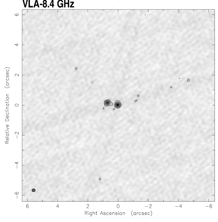
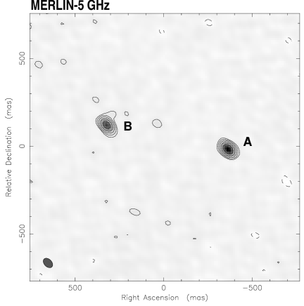
B1127+385 was observed on 1995 August 14 with the VLA in A-array at 8.4 GHz as one of the $\sim$10,000 flat spectrum CLASS sources. The image shows two compact components separated by $\sim$0.7 arcsec (Fig. 1). The 92-cm (0.327 MHz) WENSS (de Bruyn et al., in preparation) flux density is $12\pm 3$ mJy, establishing a slightly inverted radio spectrum. This implies that both components, with similar flux density at 8.4 GHz, most likely have a flat or inverted spectrum. This immediately made B1127+385 a strong lens candidate, because a change alignment within 0.7 arcsec of two unrelated compact flat spectrum radio sources is less than $10^{-6}$. Thus there is only a probability $<$1 per cent of finding such a change alignment in the sample of $\sim$10,000 flat spectrum sources. No indication of variability has been found sofar. A MERLIN 1.7 GHz long-track observation on 1996 February 13 showed two compact components. Subsequently, a snapshot observation with MERLIN was made at 5 GHz in 1996 December. These observations show only the two compact components A and B (Fig. 1). The VLA and MERLIN observations were reduced in AIPS and mapped by the Caltech package DIFMAP (Pearson et al. 1994; Shepherd 1997). The flux densities and positions were determined in DIFMAP by fitting Gaussian models to both components simultaneously. The results are listed in Table 1. The spectral indices of the components are $-0.08$ (A) and 0.05 (B) ($S_{\nu}\propto\nu^{\alpha}$) respectively between the VLA 8.4 GHz and MERLIN 5 GHz flux densities, and $-0.05$ (A) and $-0.11$ (B) respectively between the VLA 8.4 GHz and MERLIN 1.7 GHz flux densities. The errors on these spectral indices are $\sim 0.15$. The compactness and similarity in spectral index of both radio components underline the lens candidacy of B1127+385. But high resolution radio observations and optical follow-up are necessary to secure its lensing nature.

Table 1: VLA 8.4 GHz (1), MERLIN 5 GHz (2), MERLIN 1.7 GHz (3) and VLBA 8.4 GHz (4) astrometry and flux densities for B1127+385. The integrated flux densities from the VLBA observations are given. The VLBA positions of A1 and B1 are $11^{\rm h}30^{\rm m}0.099^{\rm s},$ $+38^{\circ}12^{\prime}3.091^{\prime\prime}$ and $11^{\rm h}30^{\rm m}0.157^{\rm s},$ $+38^{\circ}12^{\prime}3.232^{\prime\prime}$ (J2000), respectively. The errors on the flux densities are $\sim$10 per cent. All errors are $1\sigma$.

	$\Delta\alpha({\rm mas})$	$\Delta\delta({\rm mas})$	$S_{\nu}({\rm mJy})$	Instr.
A	$0\pm 5$	$0\pm 5$	14.7	(1)
	$0\pm 2$	$0\pm 2$	15.3	(2)
	–	–	16.0	(3)
A1	$0.0\pm 0.1$	$0.0\pm 0.1$	13.7	(4)
A2	$0.6\pm 0.1$	$2.1\pm 0.1$	$|$
B	$688\pm 5$	$145\pm 5$	11.8	(1)
	$685\pm 2$	$138\pm 2$	11.5	(2)
	–	–	14.0	(3)
B1	$686.6\pm 0.1$	$140.1\pm 0.1$	10.8	(4)
B2	$687.0\pm 0.1$	$139.2\pm 0.1$	$|$

2.2 VLBA observations

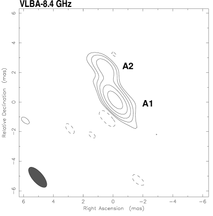
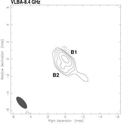
VLBA 8.4 GHz observations were made on 1996 November 4. Phase referencing was used, switching between B1127+385 (4 min integration) and the strong nearby JVAS phase-reference source B1128+385 (Patnaik et al. 1992; 2 min integration) for a period of 3.5 hours. The map of B1128+385 shows a sub-mas unresolved point source at 8.4 GHz. Fringe-fitting (Thompson, Moran & Swenson 1986) was therefore performed on B1128+385 and the solutions were directly transferred to B1127+385, which is $\sim$11 arcmin west of B1128+385. All data reduction was performed in AIPS and mapping was done in DIFMAP. The data was uniformly weighted. The resulting map resolution is $1.7\times 0.7$ mas (PA of $41^{\circ}$).

Components A and B show clear evidence for the presence of substructure (Fig. 1). Model fitting in DIFMAP shows that two axisymmetric Gaussian components can well represent the substructure in images A and B. The positions of the Gaussian components and their flux densities are listed in Table 2 for their best fit (minimum $\chi^{2}$). The separation between A1 (A2) and B1 (B2) is 700.7 (700.0) mas and the position angle of the line from A1 to B1 is $78.5^{\circ}$. The flux density ratios between A1 and B1, and A2 and B2 are 1.3 and 1.1, respectively. The integrated flux density ratio of A over B is 1.3, consistent with the 8.4 GHz VLA (1.3) and 5 GHz MERLIN (1.3) flux density ratios. The large position angle difference of $\sim 139^{\circ}$ between the subcomponents in A and B is expected if A and B are lensed and given opposite parities (Schneider, Ehlers & Falco 1992).

Table 2: The separations and position angles (north to east) of components A2 (B2) with respect to components A1 (B1). The flux densities are those of (A1, A2) and (B1, B2), respectively. The errors on the flux densities are $\sim 10$ per cent. All errors are $1\sigma$.

	Sep. (mas)	P.A. (∘)	$S_{\rm 8.4GHz}$ (mJy)
A	$2.20\pm 0.15$	$16\pm 4$	10.5,3.2
B	$0.97\pm 0.15$	$155\pm 9$	7.9,2.9

3 HST observations

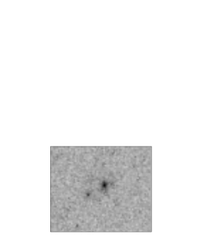
Hubble Space Telescope (HST) exposures of B1127+385 in the filters F555W ($V$) and F814W ($I$) were taken on 1996 June 21, using the Wide Field Planetary Camera (WFPC2). The exposures were taken on the PC chip (45.5 mas pixel^-1) and the exposure times in $V$ and $I$ band were $700{\rm s}+300$s and $2\times 500$s, respectively. A standard reduction was performed on both images. The $I$-band image is shown in Fig. 2. The $I$-band image shows two clear emission peaks within $\sim$1 arcsec distance from the radio components. Except for a bright nearby galaxy 8 arcsec south, no other galaxies are seen near B1127+385. Because the absolute astrometry of the HST is poorly matched (offsets of $\sim$1 arcsec) to the more accurate VLBI astrometry, we cannot ‘blindly’ overlay the optical and radio maps. However, the contour plot of the optical $I$-band emission, convolved to 0.1 arcsec (Fig. 3), clearly shows two bright (G1 and G2) and one fainter emission feature. If we assume that the radio component A is associated with the optical emission ($\sim 9\sigma$ peak) west of G1, we find that also radio component B is associated with an emission feature ($\sim 5\sigma$ peak). Although there appears to be a slight offset between the optical emission and the radio position of B, this could be due to the poorer signal-to-noise or the extended nature of the optical emission near B.

Figure 2: HST $I$-band image of B1127+385. The two radio components are associated with two emission features west (A) and east (B) of G1 (see also Fig. 3). North is up, east is left. The area shown is 3.1 arcsec $\times$ 2.6 arcsec.

Both G1 and G2 are extended, suggesting that both are galaxies. Photometry and relative astrometry were performed on G1 and G2 in $I$ band, and only photometry in $V$ band (Table 3). The $V-I$ colour indices of G1 and G2 are 1.9 and 2.0 mag, respectively. The separation is 0.60 arcsec and the position angle of the line G1-G2 is $120^{\circ}$.

Table 3: HST relative astrometry ($I$ band) and photometry for B1127+385. Component G1 is located at $11^{\rm h}30^{\rm m}0.1726^{\rm s}$, $+38^{\circ}12^{\prime}1.903^{\prime\prime}$ (according to the stsdas/metric routine in IRAF). All errors are $1\sigma$.

	$\Delta\alpha({\rm mas})$	$\Delta\delta({\rm mas})$	$I$ (magn.)	$V$ (magn.)
G1	$0\pm 5$	$0\pm 5$	$22.5\pm 0.1$	$24.4\pm 0.2$
G2	$521\pm 5$	$-299\pm 5$	$23.5\pm 0.1$	$25.5\pm 0.2$

Figure 3: Contour plot of B1127+385. The HST image has been convolved to 0.1 arcsec to bring out the optical emission more clearly. The two markers show the radio positions of A and B, where A has been placed on the centre of the optical emission as determined by a Gaussian fitting procedure. The contours indicate $(3,6,9,12,15,18,21)\times{\rm rms}$ noise in the image.

4 Modelling

In this section we present a model that reproduces the observed properties of B1127+385. We use a Singular Isothermal Ellipsoid (SIE) mass distribution (Kormann, Schneider & Bartelmann 1994) to describe the lens galaxies. We assume a smooth FRW universe. If not mentioned otherwise, all errors indicate 99 per cent confidence intervals.

From the VLBA observations we obtain 10 constraints (8 from the image positions and 2 from the flux density ratios). The two source positions give 4 free parameters and the mass model gives 3 (velocity dispersion, surface density (SD) axis ratio and position angle). The number of degrees of freedom (NDF) is therefore 3.

4.1 Single lens mass model

Initially we try a model consisting of a single SIE galaxy. We place the mass distribution on the surface brightness (SB) centre of G1, determined by fitting a 2D-Gaussian profile to it. The position of G1 relative to the optical emission feature associated with radio component A is $(-0.228^{\prime\prime},-0.038^{\prime\prime})$, with a $1\sigma$ error of $\sim$5 mas in both $x$ and $y$. The parities of components A and B are taken as –1 and +1, respectively. Choosing +1 and –1 for A and B, and letting the centre of the SD distribution move freely, give in all cases (both for the single and double lens case) unsatisfactory models ($\chi^{2}\ga 5$).

Using the image positions and flux density ratios of the radio components from Tables 1 and 2, we project rays back on the source plane through the lens. For the two image pairs – A1&B1 and A2&B2 – we simultaneously minimize the distance between the back-projected rays and the difference between observed and model flux density ratios (Kayser 1990). We allow for a $1\sigma$ error of 0.1 mas in the relative $x$ and $y$ distances between the positions of the two back-projected rays and their average position. A $1\sigma$ error of 0.15 is allowed for the flux density ratios. When the model has converged sufficiently, we use the average source positions to calculate the image positions in the lens plane. These are subsequently used to calculate a $\chi^{2}$ from the mismatch with the observed image positions. The resulting mass model parameters for minimum $\chi^{2}$ (lens plane) are listed in Table 4 (model I).

4.2 Double lens mass model

Although G1 is the primary lens, G2 cannot be neglected as it lies close to G1 and is only $\sim$1 mag fainter. We therefore extend the model by placing a Singular Isothermal Sphere (SIS) at the position of G2 — $(-0.749^{\prime\prime},-0.337^{\prime\prime})$ relative to component A, with a $1\sigma$ error of $\sim$5 mas in $x$ and $y$. We choose a SIS for G2, because G2 is only an external perturber of the primary lens G1 and as long as there is no need to complicate the model (poor $\chi^{2}$) one should keep the mass model as simple as possible. Using a SIE for G2 would add two extra free parameter (axis ratio and position angle) and make the mass model less constrained.

The velocity dispersion of G2 is fixed at $0.79\cdot\sigma_{\parallel}^{\rm G1}$, using $L\propto\sigma_{\parallel}^{4}$ (e.g. Faber & Jackson 1976) in combination with the $\sim$1 mag difference between G1 and G2 and assuming they have similar mass-to-light ratios. We repeat the $\chi^{2}$ minimization procedure. The resulting model parameters are listed in Table 4 (model II). Model II reproduces the relative positions of all four images to within 0.08 mas, compared to 0.16 mas for model I. And although the number of degrees of freedom does not change between models I and II, the reduced $\chi^{2}$ of model II is significantly smaller than that of model I. A reduced $\chi^{2}>4.5$ corresponds to a probability of $4\cdot 10^{-3}$ and model I can therefore be rejected as an appropriate model with 99.6 per cent confidence. So adding G2 improves the mass model significantly. A faint image will be formed to the south-east of G2, which can be removed by a very small core radius (0.01^′′) for G2, without changing the model parameters at any signifcant level. The critical and caustic structure of model II is shown in Fig. 4, where G2 has been given a core radius of 0.01^′′.

If G1 and G2 are spiral galaxies, the relation between luminosity and velocity dispersion is $L\propto\sigma_{\parallel}^{2.5}$ (Tully & Fisher 1977), hence $\sigma_{\parallel}^{\rm G2}\approx 0.69\cdot\sigma_{\parallel}^{\rm G1}$. The best model then has a slightly increased $\chi^{2}$ of 1.6, still a considerable impovement over model I. The resulting model parameters deviate by less than 3 per cent in velocity dispersion and axis ratio from model II. The position angle of G1 becomes $-5.3^{\circ}$, even in better agreement with the observed surface brightness position angle (see below). However, all values are well within the errors determined by Monte-Carlo simulations for model II (see Section 4.4 and Table 4).

Using a SIE for G2 would have the most influence on the position angle and axis ratio of the mass model of G1. However, the close agreement between these parameters and their observed values (see next paragraph), as well as the small resulting minimum $\chi^{2}$, indicate that adding extra free parameters is not necessary.

Figure 4: The critical curves (thick lines) and caustics (subpanel) of model II in Table 4. The star (subpanel) indicates the model position of the source as seen in the source plane. The solid contours depict the images at the positions of the radio components, if the source surface brightness is gaussian with a FWHM of 5 mas. The lens galaxy G1 is indicated by the cross-haired ellips, G2 by the cross-haired circle. The dashed contours indicate the time-delay surface for $z_{\rm d}=0.5$, $z_{\rm s}=1.5$, H₀=50 km s^-1 Mpc^-1, $\Omega_{\rm m}=1$ and $\Omega_{\Lambda}=0$.

4.3 Surface density versus surface brightness

The SD axis ratio of G1, $(b/a)_{\Sigma}^{\rm G1}=0.74$ (model II), is only slightly larger than the SB axis ratio of $0.69\pm 0.15$ that we find from fitting a 2D-Gaussian profile to the SB distribution of G1. The same Gaussian fit gives a position angle of $(-6\pm 13)^{\circ}$, close to the SD position angle of $4.9^{\circ}$. Although the SB profile of G1 is most likely not Gaussian, the position angle and axis ratio inferred from a 2D-Gaussian fit will give a good indication of the value for these parameters.

Strong evidence that B1127+385 is a gravitational lens system is given by the expected centre of the SD distribution of G1. In Fig. 5 the 99 per cent confidence contour of the central SD position of G1 is plotted. The two circles indicate the radio components A and B. If we assume that the two faint optical emission features are associated with A and B, we find that the optical emission peak of G1 (cross) falls perfectly inside the 99 per cent confidence contour. In other words, the position of the SB centre of G1 relative to the faint emission feature west of it coincides with the position of the SD centre of G1 relative to radio component A. This suggests G1 and G2 are indeed two lens galaxies and the faint optical emission features (Fig. 3) are associated with the radio components.

4.4 Monte-Carlo simulations

To investigate the overall reliability of model II, we performed Monte Carlo simulations. We minimize $\chi^{2}$ for 10,000 models, where we add Gaussian distributed errors ($1\sigma$) to the relative image positions (0.1 mas), flux density ratios (0.15), galaxy positions (5 mas) and velocity dispersion ratio between G1 and G2 (0.10).

4.4.1 Mass model parameters

The parameter probability density distributions of all models with $\chi^{2}<11.3$ (99 per cent confidence interval) are shown in Fig. 6. The figure also shows the 99 per cent confidence interval (shaded) of the observed SB axis ratio and position angle. We see that the probability distributions of both the SD axis ratio and position angle have considerable overlap with these shaded regions. Hence, the axis ratio and position angle of the luminous matter agree well with those inferred from the SD distribution of G1. The mean values of the recovered position angle and separation of A1 relative to A2 are $(18\pm 7)^{\circ}$ and $2.0\pm 0.2$ mas and for B1 relative to B2 $(163\pm 3)^{\circ}$ and $1.1\pm 0.2$ mas, where the errors are the rms values of the parameter probability distributions. These recovered model parameters compare well with the observed values listed in Table 2. We consider this as strong evidence for the validity of the lens model.

To investigate the ratio $(\sigma_{\parallel,\rm G2}/\sigma_{\parallel,\rm G1})$, we calculate the minimum $\chi^{2}$ for a range of this ratio, as shown in Fig. 6. The two horizontal lines indicate the 90 per cent and 99 per cent confidence intervals of the $\chi^{2}$ distribution. The shaded region indicates the 99 per cent confidence interval for the ratio $(\sigma_{\parallel,\rm G2}/\sigma_{\parallel,\rm G1})$, determined above. The dot gives the ratio we determined from the $\sim$1 mag luminosity difference. We see that this ratio lies well below the 99 per cent confidence level, which shows that the ratio expected from the mass model agrees with that determined from the F–J relation. Also the ratio from the T–F relation agrees well.

4.4.2 Time delay

The predicted time delay between components A and B is $1.51^{+0.65}_{-0.60}\cdot f^{\rm b}_{\rm d,s}$ days (model II), where $f^{\rm b}_{\rm d,s}=(1+z_{\rm d})\cdot[D_{\rm d}D_{\rm s}/(D_{\rm ds}\;{\rm Gpc})]$ with $D_{\rm d}$, $D_{\rm ds}$ and $D_{\rm s}$ being the angular diameter distances between observer-lens, lens-source and observer-source, respectively and $z_{\rm d}$ the redshift of the lens. For typical lens (0.5) and source (1.5) redshifts, the delay is around $7/h_{50}$ days (flat universe with $\Omega_{\rm m}=1$). The velocity dispersion of G1 is $97.6^{+5.4}_{-5.4}\cdot f^{\rm a}_{\rm d,s}$ km s^-1 (model II), where $f^{\rm a}_{\rm d,s}=\sqrt{{D_{\rm s}}/{D_{\rm ds}}}$. The errors indicate the 99 per cent confidence interval, inferred from the Monte-Carlo simulations. The 68 per cent (1$\sigma$) confidence intervals are $\sim$2.5 times smaller. Both the velocity dispersion and time delay depend on the chosen cosmological model through the angular diameter distances. A good description of the dependence of the model time delay and the angular diameter distances on the cosmologcal model is given in Helbig (1997). In a flat universe ($\Omega_{\rm m}+\Omega_{\Lambda}=1$) the difference in time delay is $\la$10 per cent between $\Omega_{\rm m}=1$ and $\Omega_{\rm m}=0.3$. For a non-flat universe significant ($\gg$10 per cent) differences in time delay are possible, depending on the clumpiness of matter and the combination of $\Omega_{\Lambda}$ (normalised cosmological constant) and $\Omega_{\rm m}$ (matter density). All other parameters in Table 4 are dimensionless and independent of the cosmological model.

We conclude that model II is in substantial agreement with all available radio and optical observations of B1127+385. However, more detailed studies of the SB distributions of G1 and G2 are necessary to improve the models and tighten the confidence intervals. Moreover both lens and source redshifts are unknown.

Table 4: The minimum$-\chi^{2}$ mass model parameters for B1127+385. Listed are the SD axis ratio $(b/a)_{\Sigma}$, the velocity dispersion $\sigma_{\parallel}$, the position angle (PA) of the major axis and the centre $(x,y)_{\rm G1}$ of G1 and the position and velocity dispersion of G2. The errors on axis ratio, velocity dispersion and position angle indicates the 99 per cent confidence interval inferred from Monte-Carlo simulations (Fig. 6). $(x,y)_{\rm src1/2}$ give the source positions of the subcomponents A1&B1 and A2&B2, respectively. Furthermore, $r_{A/B}$ and $\mu_{\rm A,B}$ give the derived flux density ratios and image magnifications. The coordinate system has been centered on image A1. The definitions of $f^{\rm a}_{\rm d,s}$ and $f^{\rm b}_{\rm d,s}$ are given in Section 4.4.2.

	Model I	Model II
$(b/a)_{\Sigma}^{\rm G1}$	0.56	$0.74^{+0.10}_{-0.12}$
$(x,y)_{\rm G1}$ (mas)	(-228.0,	(-228.0,
	-38.0)	-38.0)
$\sigma_{\parallel}^{\rm G1}$ (km s-1)	$108.9\cdot f^{\rm a}_{\rm d,s}$	$97.6^{+5.4}_{-5.4}\cdot f^{\rm a}_{\rm d,s}$
PAG1 (∘)	-26.4	$4.9^{+28.2}_{-22.4}$
$(x,y)_{\rm G2}$ (mas)	—	(-749.0,
	—	-337.0)
$\sigma^{\rm G2}_{\parallel}$ (km s-1)	—	$0.79\cdot\sigma_{\parallel}^{\rm G1}$
$(x,y)_{\rm src1}$ (mas)	-350.20$\pm$0.03,	-439.81$\pm$0.03,
	-1.10$\pm$0.07	-113.94$\pm$0.02
$(x,y)_{\rm src2}$ (mas)	-350.38$\pm$0.03,	-439.89$\pm$0.03,
	-1.62$\pm$0.07	-114.42$\pm$0.02
$r_{\rm B1/A1}$	0.56	0.71
$r_{\rm B2/A2}$	0.57	0.71
$\mu_{\rm A1,A2}$	-3.73	-4.65
	-3.66	-4.60
$\mu_{\rm B1,B2}$	2.09	3.28
	2.09	3.28
$\Delta t_{(\rm\tiny B1-A1)}$ (days)	$2.64\cdot f^{\rm b}_{\rm d,s}$	$1.51^{+0.65}_{-0.60}\cdot f^{\rm b}_{\rm d,s}$
$\chi^{2}/{\rm NDF}$	4.5	1.1

Figure 5: The 99 per cent confidence contour of the central SD position of G1, determined only on the basis of the VLBA radio images. The cross gives the 99 per cent confidence region of the SB distribution of G1 relative to the optical component west of it. The two circles indicate the two radio components, assuming they are associated with the optical emission features (see text). With this assumption, the SB centre of G1 is in excellent agreement with its inferred SD centre.

Figure 6: From upper left to lower right: Monte-Carlo probability density distributions (of models with $\chi^{2}<11.3$; 99 per cent confidence interval) of $\sigma_{\parallel,\rm G1}$, $(b/a)_{\Sigma,\rm G1}$ and P.A._G1. The shaded regions (99 per cent confidence interval) indicate these parameters as derived from the SB distribution of G1. The lower right panel shows $\chi^{2}$ as function of $(\sigma_{\parallel,\rm G2}/\sigma_{\parallel,\rm G1})$. The observationally derived ratio falls well within the region containing 90 per cent of the $\chi^{2}$ distribution.

4.5 Galaxy colours, luminosities and ${\rm M}/{\rm L}$ ratios

Having convinced ourselves that G1 and G2 are the lens galaxies, we compare their colours (F555W–F814W$\approx$1.9–2.0) with the synthesized galaxy colours in Fukugita, Shimasaku & Ichikawa (1995). For the different galaxy types approximate photometric redshifts of 0.3 (E), 0.4 (S0), 0.4 (Sab), 0.7 (Sbc) and 0.9 (Scd) are found. G1 and G2 could therefore be early type galaxies (including Sab) at low redshift (0.3–0.4) or late type galaxies at high redshift (0.7–0.9). The integrated luminosities of G1 and G2 in $B$ band for the different types of galaxies are: $\log_{10}(L_{{\rm B}\odot})\approx 8.4-2\log(h_{50})$ (E), $8.8-2\log(h_{50})$ (S0 and Sab), $9.6-2\log(h_{50})$ (Sbc) and $9.8-2\log(h_{50})$ (Scd) for G1 (${\rm H}_{0}=50\cdot h_{50}$ km s^-1 Mpc^-1), where we used the photometric redshifts found above and the $B$–F814W colours and K corrections from Fukugita et al. (1995). For G2 these values are 0.4 lower.

At a redshift $z_{\rm d}=0.3$, $I$=22.5 (G1) corresponds to an absolute magnitude $M_{I}\sim-19-5\log(h_{50})$. For an E and S0 type galaxy this would mean it is $\sim$4 mag underluminous compared to E and S0 type galaxies in the Hubble Deep Field (Mobasher et al. 1996). Placing the galaxy at higher redshifts would make the $V-I$ colours of G1 and G2 inconsistent with those of E or S0 type galaxies (Fukugita et al. 1995). The absolute $I$ magnitude is consistent however with somewhat later type spiral galaxies at higher redshifts ($z_{\rm d}\ga 0.5$). This would also explain why the velocity dispersions of G1 and G2 appears significantly smaller than those expected for $L_{*}$ E and S0 type galaxies (e.g. Kochanek 1993, 1994).

Using the velocity dispersions listed in Table 4 (model II), the mass-to-light ratios (using the mass inside the Einstein radius, the photometric lens redshifts and the total B luminosity) of G1 and G2 are: $(M/L_{{\rm B}})\sim 60\cdot h_{50}\;{\rm M}_{\odot}/{\rm L}_{\rm B,\odot}$ (E), $\sim 35\cdot h_{50}$ (S0 and Sab), $\sim 10\cdot h_{50}$ (Sbc) and $\sim 10\cdot h_{50}$ (Scd) (assuming $z_{\rm s}=1.5$). All of these mass-to-light ratios are significantly larger than normal galaxies of similar type, except for the higher redshift late-type spiral galaxies. Dust obscuration could increase the mass-to-light ratio, however it would also make the F555W–F814W colours less reasonable.

We should note however that at intermediate redshift an error of 0.2 in redshift introduces $\sim$1 mag error in B and as mentioned, dust obscuration (e.g. B1600+434; Jaunsen & Hjorth 1997; Koopmans, de Bruyn & Jackson 1998) or luminosity evolution (e.g. Bender, Ziegler & Bruzual 1996; Hudson et al. 1998) have not been taken into account.

The results above therefore give only an indication. Redshifts of G1 and G2, and more accurate colours are vital to distinguish between galaxy types and their mass-to-light ratios. To obtain the redshifts of these galaxies in a reasonable integration time, one requires an 8 or 10-m class telescope (e.g. the Very Large Telescope (VLT) or Keck).

4.6 Source

We estimate ${\rm I}\sim$24.5 for the optical emission associated with radio component A. Correcting for a magnification of 4.6 (Table 4), this corresponds to an intrinsic I$\sim$26, a luminosity of $\log_{10}(L_{{\rm I}\odot})\sim 9.8-2\log(h_{50})$ at $z_{\rm s}=1.5$ and an absolute magnitude $M_{I}\sim-19-5\log(h_{50})$ at $z_{\rm s}=1.5$ (no K-corrections applied).

Comparing this with the absolute $I$ magnitudes of galaxies in the Hubble Deep Field, the source is most consistent with a spiral galaxy of type Sbc or later, as most E and S0 type galaxies have $M_{I}\la-23$ (Mobasher et al. 1996). At a redshift of $\sim$3 the luminosity increases to $\log_{10}(L_{{\rm I}\odot})\sim 10.5-2\log(h_{50})$, still in the range of spiral galaxies (type Sab or later; Mobasher et al. 1996). We should note here that these values have not been corrected for evolution or dust absorption, internally or by the lens galaxies (G1 and G2).

However, the CLASS lens systems B0712+472 (Jackson et al. 1998) and B1933+503 (Sykes et al. 1998; Jackson, private communication) also appear to have very low luminosity sources, which could indicate that a significant fraction of the weak (few mJy) flat spectrum radio sources are associated with low luminosity objects, possibly late-type spiral galaxies.

5 Conclusions

A new gravitational lens system with two images separated by $701\pm 1$ mas has been discovered in the CLASS survey. The two radio components have a flat spectrum between 0.327 GHz (WSRT; WENSS), 1.7 GHz (MERLIN), 5.0 GHz (MERLIN) and 8.4 GHz (VLA). VLBA observations show substructure in both images. An HST $I$-band image reveals two emission features close to the radio components, which we identify with two lens galaxies. The colours and mass-to-light ratios of these galaxies seem to favour two late-type spiral galaxies at relatively high redshifts ($z_{\rm d}\ga 0.5$).

The VLBA radio structure and optical HST emission are consistent with a two-lens mass model, where a SIE and SIS mass distribution are placed on the SB centres of G1 and G2, respectively. This model is able to reproduce the separations and position angles of the VLBA substructure in radio components A and B, and their flux density ratios. Our best model has a reduced $\chi^{2}$ of 1.1. Assuming both lens galaxies are spiral galaxies, $\chi^{2}$ slightly increases to 1.6. Omitting G2 in the mass model increases the reduced $\chi^{2}$ to 4.5, which can therefore be excluded as an appropriate model with 99.6 per cent confidence.

Our best model gives a SD axis ratio of $0.74^{+0.10}_{-0.12}$, position angle of $(4.9^{+28.2}_{-22.4})^{\circ}$ and velocity dispersion of $97.6^{+5.4}_{-5.4}\cdot f^{\rm a}_{\rm d,s}$ km s^-1. The predicted time delay between radio components A and B is $1.51^{+0.65}_{-0.60}\cdot f^{\rm b}_{\rm d,s}$ days. For a typical lens (0.5) and source redshift (1.5), a time-delay of $\sim$7 days is expected for H₀=50 km s^-1 Mpc^-1 and $\Omega_{\rm m}=1$ in a flat universe. WSRT monitoring data is in hand, to see if the lensed object in B1127+385 is variable and therefore useful for determining a time-delay between the lensed images. This time-delay can constrain the Hubble parameter (Refsdal 1964). The errors on these parameters indicate the 99 per cent confidence interval of the probability density distributions found from Monte-Carlo simulations.

Having constructed a consistent model within the lensing hypothesis – explaining both the available radio and optical data of B1127+385 – it appears that B1127+385 most likely is a new gravitational lens system.

References

- [Bender, Ziegler & Bruzual1996] Bender R., Ziegler B., Bruzual G., 1996, ApJL, 463, 51
- [Faber & Jackson1976] Faber S.M., Jackson R.E., 1976, ApJ, 204, 668
- [Fukugita & Turner1991] Fukugita M., Turner E.L., 1991, MNRAS, 253, 99
- [Fukugita, Shimasaku & Ichiwaka1995] Fukugita M., Shimasaku K., Ichiwaka T., 1995, PASP, 107, 945
-
[Helbig1997]
Helbig, P., Proceedings of the Workshop on Golden Lenses, 1997,
http://multivac.jb.man.ac.uk:8000/ceres/
workshop1/proceedings.html - [Hudson et al.1998] Hudson M.J., Gwyn S.D.J., Dahle H., Kaiser N., ApJ, 503, 531
- [Jackson1998] Jackson N., et al., 1998, MNRAS, 296, 483
- [Jaunsen & Hjorth1996] Jaunsen A.O., Hjorth J., 1997, A&A, 317, L39
- [Kayser1990] Kayser R., 1990, ApJ, 357, 309
- [Kochanek1991] Kochanek C.S., 1991, ApJ, 379, 517
- [Kochanek1993] Kochanek C.S., 1993, ApJ, 419, 12
- [Kochanek1994] Kochanek C.S., 1994, ApJ, 436, 56
- [Kochanek1996] Kochanek C.S., 1996, ApJ, 466, 638
- [Koopmans1998] Koopmans L.V.E., de Bruyn, A.G., Jackson N., 1998, MNRAS, 295, 534
- [Kormann, Schneider & Bartelmann1994] Kormann R., Schneider P., Bartelmann M., 1994, A&A, 284, 285
- [Mobasher1996] Mobasher B., Rowan-Robinson M., Georgakakis A., Eaton N., 1996, MNRAS, 282, 7L
- [Patnaik1992] Patnaik A.R., Browne I.W.A., Wilkinson P.N., Wrobel J.M., 1992, MNRAS, 254, 655
- [Pearson1994] Pearson T.J., Shepherd M.C., Taylor G.B., Meyers S.T., 1994, BAAS, 185, 08.08
- [Refsdal1964] Refsdal S., 1964, MNRAS, 128, 295
- [Refsdal1964] Refsdal S., 1966, MNRAS, 134, 315
- [Rhee1996] Rhee M-H., 1996, PhD Thesis, University of Groningen
- [Schneider, Ehlers & Falco 1992] Schneider P., Ehlers J., Falco E.E., 1992, Gravitational Lenses, Springer Verlag, Berlin
- [Shepherd1997] Shepherd M.C., 1997, ADASS VI, A.S.P Conference Series, vol 125, eds., Gareth Hunt and H.E. Payne, p77
- [Sykes1997] Sykes C.M., et al., 1997, MNRAS, astro-ph/9710358
- [Thompson1986] Thompson A.R., Moran J.M., Swenson G.W., 1986, Interferometry and Synthesis in Radio Astronomy, Wiley-Interscience publication, p262
- [Tully1977] Tully R.B., Fisher J.R., 1977, A&A, 54, 661