A Deep Survey of HI–Selected Galaxies:
The Sample and the Data

Abstract

In a 21 cm neutral hydrogen survey of approximately 55 deg² out to a redshift of $cz=8340$ km s^-1, we have identified 75 extragalactic HI sources. These objects comprise a well-defined sample of extragalactic sources chosen by means that are independent of optical surface brightness selection effects. In this paper we describe the Arecibo survey procedures and HI data, follow-up VLA HI observations made of several unusual sources, and Kitt Peak $B$-, $R$-, and $I$-band photometry for nearly all of the galaxies. We have also gathered information for some of the optically detected galaxies within the same search volume.

We examine how samples generated by different types of search techniques overlap with selection by HI flux. Only the least massive HI object, which is among the lowest mass HI sources previously found, does not have a clear optical counterpart, but a nearby bright star may hide low surface brightness emission. However the newly-detected systems do have unusual optical properties. Most of the 40 galaxies that were not previously identified in magnitude-limited catalogs appear to be gas-dominated systems, and several of these systems have HI mass-to-light ratios among the largest values ever previously found. These gas-dominated objects also tend to have very blue colors, low surface brightnesses, and no central bulges, which correlate strongly with their relative star-to-gas content.

1 Introduction

A strong argument can be made that the present census of galaxies is biased toward objects which are intrinsically bright and easy to identify optically (Disney & Phillipps 1983; McGaugh 1996). Extragalactic astronomy’s historical dependence on searches of optical plates for galaxy identification almost certainly has led to an under-count of low surface brightness (LSB) objects. This bias leads to an under-representation of these objects and their properties when examining the overall extragalactic population—information which is essential when investigating the evolution of galaxies or the large-scale structure and fate of the Universe. Ridding the extragalactic census of its optical bias, or even assessing its seriousness is problematic. In this paper we present a sample of HI-selected extragalactic sources that permits us to examine the gaseous and stellar properties of galaxies in a fresh light.

Most measurable galaxy properties are in some way a direct result of stellar emission, stellar remnants, or the processes that form stars. For example, far-infrared emission from galaxies is essentially starlight re-radiated by dust grains, and the dust grains’ existence is a result of stellar evolution. Far infrared emission is therefore highly correlated with the optical emission of stars, and it is of limited utility in identifying objects that cannot easily be detected optically.

One strategy that has been used to correct the optical bias is to search for extragalactic sources at faint surface brightnesses. This was effectively begun by Nilson (1973) in the Uppsala General Catalog (UGC), where the criterion for acceptance was a minimum angular size instead of a magnitude limit. Since galaxies’ intrinsic diameters vary by a much smaller factor than do their luminosities, a diameter-limited survey detects a larger proportion of LSB galaxies. The UGC is, of course, also limited by the surface brightness sensitivity of the Palomar Observatory Sky Survey (POSS) plates (about 25 mag arcsec^-2). This has been pushed to fainter surface brightnesses by using the second generation (POSS II) plates (Schombert & Bothun 1988; Schombert et al. 1992; Pildis, Schombert, & Eder 1997). Special photographic amplification techniques that go even deeper have revealed some remarkable LSB sources like Malin 1 (Bothun et al. 1987), which has one of the largest known HI masses. However, seeking sources at ever fainter surface brightnesses becomes more and more difficult and it ultimately remains tied to the presence of starlight. It would be preferable to take an independent approach to sampling the extragalactic population.

A galaxy’s atomic hydrogen (HI) gas content is one of the few properties that should be relatively uncorrelated with its optical emission. Of course, like any extensible property of a galaxy, some degree of correlation is expected due to the galaxy’s total bulk. However, since hydrogen is primordial, it does not require star formation for its existence, and since the 21 cm line’s excitation temperature is so low, starlight is not needed to excite it. Its status as the “raw material” in star formation makes it likely that HI gas content and stellar emission will be linked in many galaxies, but since the gas is consumed in the process, the amounts may be anticorrelated. For example, it is well known that elliptical galaxies may contain little or no measurable HI, and we might also expect to find reservoirs of HI where star formation has been inefficient so that the HI emission is more readily detectable than the optical emission.

Some intriguing sources with no optical counterpart have been discovered by serendipity at 21 cm, like the ring of HI gas in Leo (Schneider 1989) and the southwest clump of the Virgo cluster cloud HI 1225+01 (Giovanelli, Williams, & Haynes 1991). The northeast clump of HI 1225+01 has a ratio of $M_{HI}/L_{B}=10$ (Salzer et al. 1991), and some other extreme objects, like DD0 154 and Malin 1, have $M_{HI}/L_{B}\approx 5$ (Carignan & Beaulieu 1989; Bothun et al. 1987). These objects represent the gas-rich extreme of a continuum of extragalactic sources that also ranges to objects that are composed almost entirely of stars, like ellipticals and dwarf spheroidal systems. The enormous range of $M_{HI}/L$ found in extragalactic sources indicates that HI properties of extragalactic sources cannot be fully appreciated from optically-selected samples.

To generate an HI-selected sample of galaxies, we have conducted a large, sensitive survey for the extragalactic 21 cm emission using the Arecibo radio telescope. Our “Arecibo Slice” covers about 1^∘ in declination and a total area of about 55 sq deg out to a redshift of $cz_{hel}=8340$ km s^-1. We also examine the literature for optically-selected sources that reside in our survey volume. Most of these were “rediscovered” by the 21 cm survey, but we have attempted to track down other galaxies from magnitude-limited and other types of catalogs.

In addition, we have collected multi-wavelength optical data to allow color and luminosity comparisons. We have also observed several of the most unusual galaxies detected in the survey with the VLA in order to examine their HI sizes, and better-determine their positions. In this paper we present these data and examine the differences, overlaps, and similarities of the gaseous and stellar properties of our sample galaxies.

Our survey has been more successful than previous searches at identifying low mass HI sources and has found a substantial population of objects whose gas content dominates over their stellar content. Among our 75 HI-selected sources is one of the lowest mass field HI sources found to date, with an HI mass similar to M81 dwarf A found by Lo & Sargent (1979) in an HI survey of that nearby group. Based on optical data collected at Kitt Peak, seven of our objects have $M_{HI}/L_{B}>3$, which was the value found for M81 dwarf A (Sargent, Sancisi, & Young 1983). A dozen of our objects also have substantially bluer colors than any of the HI-detected galaxies studied by Szomoru et al. (1994), or in diameter-limited samples of galaxies like de Jong & van der Kruit (1994).

In large part, this survey’s success results from the size of the volume examined. This is a useful starting point for comparing surveys and is illustrated in Fig. 1. We show the volume within which various “blind surveys” (not based on earlier optical imaging) have been potentially sensitive to an HI source of a given mass. This is an approximation based on the area examined, the quoted $rms$ noise, redshift range covered, and sensitivity across the bandpass for each survey (see Schneider 1997 for more details about the surveys). This graph assumes the HI sources all have the same velocity width, and that the search techniques are all equivalent. In fact, though, detection rates are influenced by a wide variety of factors that can be difficult to quantify.

Figure 1: Comparison of mass–volume sensitivity of various “blind” HI surveys. The lines indicate the approximate volume within which a source of a given HI mass could have been detected based on the survey’s resolution, bandpass, noise level, and areal coverage. See Schneider (1997) for details of the different surveys.

Early surveys with the Green Bank 300 foot telescope by Shostak (1977) and Fisher & Tully (1981) were limited by receiver sensitivity and the total bandpass available. Krumm & Brosch (1984) surveyed a large volume by searching at higher redshifts, but they were then insensitive to low mass sources. With improved receiver systems, Henning (1990, 1995) was able to search within larger volumes over a wide range of masses. The Green Bank 300 foot telescope was in many ways an ideal survey instrument because the main limitation to search efficiency is, in principle, the system temperature of the receiver system (see, for example, Schneider 1996), which was excellent at the 300 foot telescope.

A smaller-beam telescope has the advantage of avoiding confusion, which is important because of galaxies’ tendency to cluster. This is particularly demonstrated by a survey conducted using the VLA (Weinberg et al. 1991; Szomoru et al. 1994), which searched a volume comparable to some of the early surveys. They identified nine previously uncataloged sources, but six of these were in the neighborhood of bright cataloged galaxies and might well have been assumed to be part of these galaxies if surveyed with the $\sim 11^{\prime}$ beam of the Green Bank 300 foot telescope. The VLA also has advantages for interference rejection, but sensitivity and bandpass limitations at the VLA constrain the amount of volume it can search. The restriction on bandpass is the reason why the sensitivity of the VLA survey drops off sharply below $10^{8}M\sun$.

The Arecibo radio telescope represents a good compromise. Its $\sim 3.3^{\prime}$ beam would have confused only one of the VLA-identified sources, and it provides a wide bandpass with adequate spectral resolution to detect narrow-line HI sources. As shown in Fig. 1 we examined a substantially larger volume at low HI masses than any of the Green Bank or VLA surveys. A recent “Arecibo HI Strip Survey” or AHISS by Sorar (1994; also see Zwaan et al. 1997) used a drift scan strategy to sample a similar-sized volume. Not counting sidelobes, that survey actually covered about a third as much area on the sky, but the quoted $rms$ noise levels suggest it should be sensitive over a slightly larger volume for low mass HI sources. The methodology of our survey is different from the AHISS, which might account for our higher detection rate of low-mass HI sources despite the nominally smaller search volume. This is a crucial point for determination of the HI mass function, and we discuss it at greater length in a subsequent paper (Schneider, Spitzak, & Rosenberg 1998) where we apply tests to determine sample completeness.

In this paper we begin in §2 with a description of the survey techniques and the Arecibo and VLA HI data. In §3 we describe the optical data and cross-identifications of our sources with other catalogs. In §4 we focus on distance-independent properties of the galaxies, with a particular interest in understanding the selection effects that determine which galaxies are included in which types of surveys. Finally, in §5 we conclude with a summary of our results, highlighting some of the most unusual individual objects that deserve follow-up observations. We will analyze the intrinsic distance-dependent properties of the galaxies, including their luminosity function, in subsequent papers.

2 The HI Survey

2.1 21 cm Observations

The 21 cm survey observations were conducted at the Arecibo radio telescope using the “22 cm” feed. The Arecibo telescope has the largest collecting area and highest resolution of any single-dish 21 cm telescope. The telescope response has a strong zenith-angle dependence, and our search strategy was largely dictated by this limitation. In addition, because this survey would require a large amount of observing time with little idea of the detection rate, we selected a right ascension range where there was relatively low “proposal pressure”: the portion of the southern Galactic cap accessible from Arecibo. Optically-identified sources in this region have been extensively studied by Giovanelli & Haynes (1993, and references therein), leaving relatively less demand for telescope time from $22^{h}$ to $4^{h}$.

To optimize the survey we also needed to observe a region within the 10^∘ zenith angle of the telescope’s maximum sensitivity. And to provide some transit time at full sensitivity this could be at most about $8^{\circ}$. At the same time, we wanted to avoid the $\sim 3^{\circ}$ closest to zenith where the telescope can have difficulty tracking a source. For the observatory’s $18^{\circ}21^{\prime}$ latitude, this gave us a choice of $21^{\circ}21^{\prime}<\delta<26^{\circ}21^{\prime}$ or $10^{\circ}21^{\prime}<\delta<15^{\circ}21^{\prime}$. Although the southern choice has the advantage of being farther from the Galactic plane, we chose the northern side because much more HI data had been published in that area (Giovanelli & Haynes 1989; Giovanelli et al. 1986). These previous HI observations allow us to test our completeness.

The “Arecibo Slice” is within the region $22^{h}00^{m}<\alpha(1950)<03^{h}24^{m}$ and $22^{\circ}58^{\prime}<\delta(1950)<23^{\circ}47^{\prime}$, although in the portion of right ascension earlier than $22^{h}54^{\prime}$, the survey reached a maximum declination of $23^{\circ}19^{\prime}$ (Fig. 2). Overall, close to $55$ deg² were surveyed in 14,130 pointings of the telescope. The positions observed were separated by $4.1^{\prime}$ on a hexagonal (“honeycomb”) grid. A hexagonal grid is preferable to a rectangular grid because there is less sensitivity variation for sources off beam center (Schneider 1989). The 22 cm feed has a beam size of $3.3^{\prime}$ (FWHM), so the gain would be about 4$\times$ smaller than its value at beam center for a source in the worst possible position on the grid. However, for extended sources the gain variations are smaller, and sources between beams might be detected at neighboring grid points, so the sensitivity probably varies by less than a factor of three anywhere in the survey region.

Figure 2: Region surveyed in the Arecibo HI slice. Positions of galaxies in the RC3 with redshifts in the range of the survey (100–8340 km s^-1) are marked by $\times$ symbols. The region around $\delta=23^{\circ}$ covered by the HI survey is shown by an outline. The serpentine ridge north of the slice is the Pisces–Perseus supercluster at approximately 5000 km s^-1, and the higher density of galaxies around $\alpha=2^{h}$ is part of the supergalactic plane.

At each point a one minute integration was made over a bandwidth corresponding to redshifts of $100<cz_{hel}<8340$ km s^-1. This nominally corresponds to distances between 1.3 and 111 Mpc for a Hubble Constant of 75 km s^-1 Mpc^-1 (assumed throughout this paper) and a total survey volume of $\sim$7630 Mpc³. We tuned the 22 cm feed to its highest tunable frequency, corresponding to a redshift of $cz_{hel}=5300$ km s^-1, for these observations. The sensitivity rolled off to 81% of its maximum at the high-redshift end of the bandpass, and 56% at the low-redshift end.

During a given observing run, points on the hexagonal grid spaced by $1^{m}12^{s}$ were observed in sequences of 15. The offset nearly equaled the integration plus slew time between points so that the telescope remained in a nearly fixed configuration. Because sources are uncommon, the other 14 observations in a sequence could be combined to make a low noise “off” (calibration) scan, and the noise in the final spectrum comes almost entirely from the “on” scan alone. This mapping method is about four times more efficient than the standard position-switching procedure for a single point, which would require 2 min “on” plus 2 min “off” to reach a similar noise level.

The autocorrelation spectrometer channels were spaced by 39 kHz ($\sim 8.2$km s^-1). After Hanning smoothing the resolution was $\sim 16.4$km s^-1 giving us undiminished sensitivity to sources with line widths as narrow as $\sim 32$km s^-1, which is about as narrow a velocity spread as any dwarf galaxy is known to have. After carrying out a polynomial fit to channels away from interference or signals, the noise was typically 1.7 mJy. With corrections for the frequency response of the feed, the average noise across the band was about 2.0 mJy.

2.2 Signal Identification

Both software techniques and visual examination were used to identify possible signals in each spectrum. The software techniques included a range of velocity smoothings and a variety of interference identification and rejection schemes. The dominant problem was the rejection of weak sources of interference. Strong interference was relatively easy to isolate because it would normally persist for more than one minute; thus it would appear in neighboring spectra in time, but these were separated by 4 beam spacings ($\sim 16^{\prime}$) on the sky and unlikely to be real sources. We also identified interference by comparing the left and right circular polarizations; most man-made signals will appear polarized while HI emission does not.

Weak interference was much more difficult to isolate because polarization might be indistinguishable from noise variations, and it might only exceed the search threshold level in an isolated spectrum. In the end, the by-eye search proved to be the more effective method for identifying weak signals—the software methods could be adjusted to identify weak signals, but only at the expense of introducing very large numbers of spurious sources. We suspect this is because of a variety of subtle visual cues that are difficult to design into software recognition, like artifacts of baseline removal, experience of past patterns of interference, or knowledge of the probable shape of HI profiles. Of course, these same cues represent potential biases against non-standard sources of HI emission, and this should be kept in mind when trying to understand the completeness of the survey.

Overall, we identified 230 positions by eye or by software algorithms with suspected emission, and these were re-observed with standard “on–off” integrations, except for cataloged sources that had already been detected at our position and redshift. (Note, though, that information about previous detections was not consulted before carrying out our searches.) For the suspected signals that we did reobserve, our confirmation rate was about 30%. Genuine HI signals were confirmed at 101 of the 14,130 survey positions. These correspond to only 75 distinct sources since some sources were detected at neighboring positions, and at some positions more than one HI source was evident. We also dropped one galaxy (UGC 1551) from the final sample even though it generated a genuine HI signal because it was outside of the survey area and was detected through a sidelobe in an observation along our northernmost row.

In order to determine their fluxes and positions more precisely, all 75 of the HI-selected sources were mapped in more detail. We designed an observing pattern to examine a central point and six equally-spaced surrounding positions, 2.3^′ away from each other, for one minute each. A single “off” position was tracked for 5 min at the average configuration of the telescope during the seven “on” scans. For each source, we fit a simple model to the integrated fluxes at the seven positions of the hexagonal maps. We treated each as an elliptical-shaped Gaussian distribution of gas with an unknown size, position, and orientation on the sky and model the beam as a Gaussian with a FWHM of 3.3^′.

The HI source number and best-fit coordinates of the HI are listed in Table 1, columns (1) and (2). Optical images (described in §3.2) centered on the HI positions are shown in Fig. 3, except for a few cases where the HI position is marked by a white $+$ symbol. Based on comparisons to the coordinates of unambiguous optical counterparts, we found that the HI positions were systematically too far south by 21^′′. This was consistent along the entire slice, so we have adjusted the declinations accordingly. The resulting centroid positions have an rms scatter of $17^{\prime\prime}$ in each coordinate relative to the optical positions, which is the approximate pointing accuracy of the Arecibo telescope.

At several mapped positions it was clear that the emission came from more than one source, based on variations of the velocity ranges and profile shapes over the area of the small hexagonal maps. In these cases (#20+#21, #22+#23, #37+#38, and #59+#60), we assigned the portion of the flux in each hexagonal map position according to its suspected source. For #20+#21 and #59+#60 the distinctions were sufficiently clear that we could fit to the HI of each source separately, and the individual coordinates are listed in Table 1. For the other two pairs, the separation was less clear, but we have made our best estimates of the individual HI parameters. We believe that all of these sources would have been individually detected if they had been isolated, and we therefore list them as separate sources in our sample. In addition, source #40 was along the northern limit of our survey, so that we did not have a good initial constraint on its position, and there seem to be some weak HI signals from nearby companions that further complicate interpretation of the small hexagonal maps. As a result we were unable to make a good estimate of its position. Because of confusion, some measurements of these sources are less certain, which we note by $\sim$ symbols before entries in the table.

For the interacting pair #22+#23 (UGC 12914+5), we consulted the VLA HI data from Condon et al. (1993) to estimate the HI properties of each galaxy. We interpret their data somewhat differently than they do based on intercomparisons of our Arecibo and their VLA maps. In particular, we examined our higher resolution spectra for edges that might correspond to the upper and lower limits of rotation in the two galaxies as mapped out in the VLA velocity-channel maps. To us it appears that UGC 12914 has HI at redshifts from 4030 to 4620 km s^-1 ranging from the northeast to the southwest. By contrast, the HI near UGC 12915 has redshifts from 4160 to 4700 km s^-1 ranging from the southwest to the northeast. This would indicate a larger velocity difference between the two galaxies than found by Condon et al. The gas is clearly asymmetrically distributed around each galaxy, with a large amount probably associated with a tidal tail extending south of UGC 12914 and a weaker excess extending northwest of UGC 12915. Our total flux of 15.75 Jy km s^-1 is in good agreement with the VLA value of 15.3 Jy km s^-1, and based on the VLA maps we estimate that 60% of the total HI emission is associated with UGC 12914 and 40% with UGC 12915.

The heliocentric redshift, and line widths at 50% and 20% of peak are listed in columns (3)–(5). The shapes of the HI profiles are shown in Fig. 3 along the bottom of each panel; the panels are 1000 km s^-1 wide.

In column (6) we indicate the “number of horns,” $N_{h}$, in each profile. Single-horn profiles are Gaussian or triangular in shape, and are usually associated with face-on galaxies or dwarfs. A two-horned profile is the signature of a rotating disk system: because the disks have a nearly constant rotation speed and are usually seen at a nearly fixed inclination, the gas clumps kinematically at two extremes. These profiles normally have steep edges and weaker emission in the center. We list $N_{h}=3$ for profiles which show an extra central peak, or which have the relatively square shape of a double-horned profile, but in which the central part of the profile is higher than the horns. These “triple-horned” profiles indicate the presence of a large amount of gas moving at lower speeds along the line of sight than the gas forming the rotation horns. This may be caused by warped disks, tidal interactions, or confusion with companions.

For normal double-horned profiles, the 50% width is the less biased estimator of galaxy rotation (Corbelli & Schneider 1997). However, in 9 instances the 50% and 20% widths vary by more than 50 km s^-1, suggesting complications that need to be considered more carefully. For source #49 the cause appears to be noise. Sources #12 and #36 have shallow-sloped edges to their profiles and are clearly interacting with near neighbors based on their optical images; some outer gas is probably orbiting at a higher inclination than the main disk. For #25 and #31, small shoulders on one side of the profile may actually be small companions. In all of these sources, the 20% linewidth would tend to be overestimated, and the 50% linewidth remains the better indicator of galaxy rotation.

The four other sources with linewidth discrepancies (#1, #4, #9, #57) are in our class of “triple-horned” profiles. For these galaxies low-velocity gas has raised the reference flux density against which the 50% comparison is made, so that it is probably measuring too narrow a line width. We would therefore recommend using the 20% line width as a better indicator of the rotation speed in these and the other triple-horned galaxies.

We list the central flux in column (7)—this is interpolated to the centroid position of the HI using our model fit to the seven positions of the small hexagonal map. We were also able to determine the total integrated HI fluxes by summing the seven spectra, weighted so that the sensitivity is nearly uniform over a $5^{\prime}$ diameter area. The total HI flux is given in column (8), and the profiles in the figure are based on these summed spectra.

2.3 Other Galaxies in the Search Volume

Using long “on–off” integrations and re-examination of the survey spectra, we also searched for HI emission from cataloged galaxies potentially within our search volume. This added 10 more sources that have 21 cm detections and 4 more with optical redshifts within the search volume. Two additional sources were also identified during follow-up HI observations in the region, making a total of 16 non-HI-selected sources in our search volume.

For six galaxies with optical redshifts (#82, #84, #87–90) we found features in the survey spectra that probably correspond to their HI emission but which we did not originally identify as part of the HI search. These all fall fairly close to our detection limit, and in the two strongest sources, interference at a nearby frequency appears to be the reason for their rejection in both the visual and software searches. The signal from source #87 is at least partially confused with the nearby pair #37+#38; we include it as a detection since there appears to be some weak emission in velocity ranges not covered by #37+#38.

Source #83 was detected during confirmation observations in the “off” scan of a suspected source. Re-examination of the search spectrum nearest its position shows weak evidence for this source, but it was again close to our detection limit. Source #91 was found during the detailed mapping of source #68, which triggered the detection, but we do not think #91 would have been detected on its own, so we include it in the non-HI-selected group.

These non-HI-selected sources provide useful checks on the limits of our survey’s sensitivity, and they provide an interesting comparison sample. We include the available 21 cm information for these sources in Table 1. Values extrapolated from observations made at nearby positions are marked with a $\sim$ symbol.

Two close companions to HI-rich galaxies had reported HI detections that we believe are due to confusion based on our own mapping. IC 1559 (#85) is just $0.4^{\prime}$ southeast of NGC 169 (#36). It has a listed HI detection in the compilation of Bottinelli et al. (1990), but we cannot identify the original source of this value. Our mapping does not show any evidence of independent HI emission from IC 1559, but higher spatial resolution is needed to make a definite determination. Similarly, IC 5242 (#76) is 2.7^′ northwest of the HI-rich IC 5243 (#3). Our map confirms the doubts of Giovanelli et al. (1986) that IC 5242 was actually detected at 21 cm. Both of these sources do have optical redshifts, though, so they remain part of our non-HI-selected sample.

Finally, we note that several sources with previous reports of HI emission generated negative results. We could not confirm the marginal detections of UGC 12663, CGCG 482-050, or IC 190 reported by Giovanelli & Haynes (1989) at redshifts that would have placed them within our search volume. Our spectra had lower rms values than theirs, and we had experienced interference at the frequency of the reported detection of UGC 12663. Since we know of no optical redshifts for these sources, we treat them as sources of unknown redshift and drop them from further consideration.

2.4 HI Detection Limits

To aid in understanding the detection statistics of our survey, in columns (9) and (10) of Table 1 we list the integrated flux and the line width at 20% of peak as determined from the original search spectra before making any corrections for frequency response or pointing. The detected flux is affected strongly by the position of the telescope beam relative to the source; the offset of the HI centroid from the nearest point on the search grid is given in column (11).

Understanding the way in which survey sensitivity depends on observational factors is essential for deriving population statistics from such a sample (Schneider 1997; Schneider et al. 1998). In principle, a source of a given integrated flux should be harder to detect if it has a wider profile since noise is added to it in proportion to the square root of the number of channels (Schneider 1996; Zwaan et al. 1997). We plot the detected fluxes against their linewidths in Fig. 4, and we show a “5–$\sigma$” detection limit based on this statistical noise argument. This is fairly good at delineating the difference between detected (solid symbols) and undetected (open symbols) sources. The boundary is somewhat fuzzy, though, and it appears that wider profiles are somewhat more difficult to detect than the statistical uncertainties alone would suggest. We explore this more thoroughly in our analysis of the HI mass function (Schneider et al. 1998).

Figure 4: Observed HI flux versus line width for sources in the Arecibo slice. HI-selected sources within our survey are shown by filled triangles and circles. Open and filled circles indicate magnitude-selected objects. Sources selected by neither criterion are marked by $\times$’s. The line shows a simple prediction of the 5–$\sigma$ detection limit for HI sources. (See text.)

Fig. 4 also introduces a notation we shall use throughout the remainder of this paper. We mark the objects detected as part of our HI-selected sample by filled symbols, and magnitude-selected sources (defined as being in any of the magnitude-limited catalogs discussed in §3.1) by circular symbols. Sources belonging to neither set are marked by $\times$ symbols. The HI-selected sample is split roughly in half between “optically-bright” HI sources (shown as filled circles) and “optically-faint” HI sources (shown as filled triangles). This division provides us with the opportunity to examine selection effects influencing the inclusion of galaxies in different catalogs. We will show in §4.2 that the optically-bright HI sources are in fact “star-dominated” while the optically-faint HI sources are “gas-dominated.”

2.5 VLA Observations

Based on the Arecibo results, several of our objects have quite extreme properties. We targeted sources #14, #17, and #75 with the VLA in D-array primarily to determine precise positions of the HI to aid in their optical identification. In addition source #18 was detected in the field of source #17.

The observations were 10 min long “snapshots” with a frequency resolution after on-line Hanning smoothing of 97.7 kHz ($\sim$21 km s^-1). The flux calibration was based on VLA standards, and for each source a nearby phase calibrator was observed at the same Doppler-shifted frequency as the HI source. The images were reduced using standard Astronomical Image Processing System (AIPS) procedures. The synthesized beams were nearly circular with $\sim 50^{\prime\prime}$ HPBW, and the rms noise was $\sim$1.4 mJy per beam.

The VLA results are given in Table 2. Coordinates are listed in column (2) and marked by white $\times$ symbols in Fig. 3. The offset from the Arecibo position is given in column (3). The AIPS Gaussian fits to the source positions quoted errors of $<1^{\prime\prime}$, but it seems more reasonable, given the beam size, to suppose an accuracy of 5–10^′′. The integrated flux, as a fraction of the Arecibo total flux is given in column (4), and the deconvolved HI dimensions in column (5).

The VLA position for source #14 indicates it is associated with an extremely low surface brightness object east of the Arecibo position. The optical data presented in §3 show that this object has the lowest surface brightness of any of our sources. The VLA and Arecibo spectra are compared in Fig. 5.

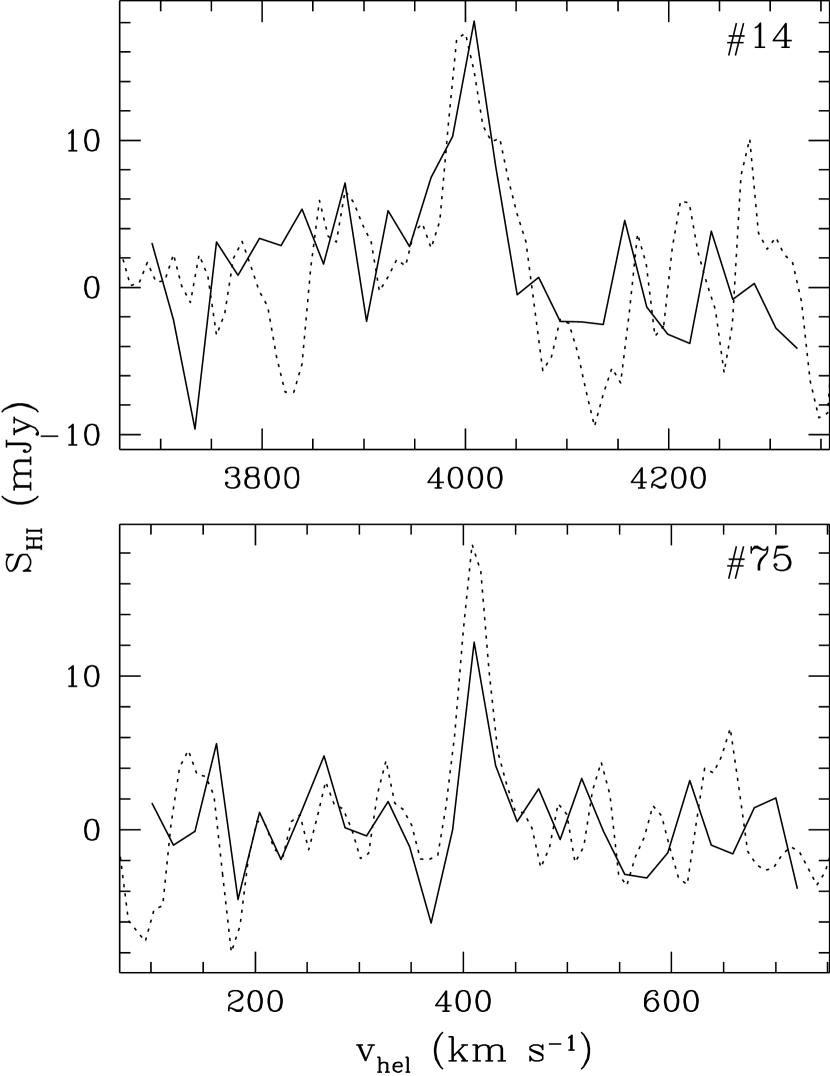
Figure 5: Comparison of Arecibo and VLA spectra for two unusual HI sources. Source #14 has the lowest surface brightness of any of our sources, while #75 has the lowest redshift and lowest mass of any of our objects. The VLA spectra are shown with a solid line, and the Arecibo spectra with a dotted line.

Source #17 is over $1^{\prime}$ south of its Arecibo position. The problem with the Arecibo position may arise from sidelobe confusion with source #18, which is 5^′ northeast of the VLA position for #17.This could also explain the substantially smaller HI flux determined at the VLA. However, the VLA detection of source #17 is concentrated almost entirely over the velocity range of the high-velocity horn seen in the Arecibo profile. This suggests that the VLA observations may not have been deep enough to detect more-extended gas associated with the main disk of the optically edge-on galaxy seen in Fig. 3. One possibility is that there may be extended tidal debris between these galaxies below our detection threshold at the VLA; this would accord with the apparent tidal tail extending to the northeast of #17 seen in the optical image.

Source #75 is the nearest and the lowest mass object detected in our survey. Based on its Arecibo position, it had no clear optical counterpart, and, unfortunately, the VLA position indicates it is 14.5^′′ south and 6.5^′′ west of the bright star in Fig. 3. The VLA and Arecibo spectra are compared in Fig. 5. The VLA flux is smaller than the Arecibo flux, although both are weak and subject to fairly large uncertainties. The Arecibo flux we give in Table 1 is the average of three separate small hexagonal maps; these maps also suggested that the source might be somewhat extended as is also suggested by the larger total flux than single-beam flux in the Table. The VLA observations indicate the HI source is point-like based on an AIPS Gaussian deconvolution of the source from the beam, so if the larger Arecibo flux is correct, there may be some extended HI emission in the region.

The VLA fluxes and deconvolved HI diameters allow us to estimate an average face-on surface density of HI in these systems. Source #14 has an estimated surface density of $2\times 10^{20}$ cm^-2, which is well below the threshold for star formation of $\sim 10^{21}$ cm^-2 found by Taylor et al. (1994). Our beam does not allow us to resolve clumping of the HI, but the smooth optical appearance suggests that the density of HI may be low throughout the disk of #14. This is in contrast to the relatively bright (although also uncataloged) source #18, which has a surface density of $9\times 10^{20}$ cm^-2 and which appears optically to have knots of star formation. Finally, since #75 is unresolved, we cannot estimate a mean column density; if we assume it is smaller than $0.5^{\prime}$, the surface density would be $>7\times 10^{20}$ cm^-2, which does not provide us with any firm indication of whether we should expect to see current star formation.

3 Optical Observations

3.1 Optical Cross-Identification

After detecting our sources, we initially searched for optical counterparts by examining the POSS. Almost all of the sources have at least one likely counterpart within a small distance of the HI position. Fig. 3 shows our own $R$-band CCD images for the HI-selected sources (see §3.2 for details of this imaging). Each field is $3^{\prime}\times 3^{\prime}$, centered on the position of the Arecibo HI detection, except #21 and #40 where the HI positions are noted by $+$ symbols.

In Table 3 we give the optical coordinates of the source we judge the most likely association in column (2). Generally this is the brightest object within $1^{\prime}$, although in regions where there is more than one candidate we have compared all of the data from the survey and hexagonal maps, noting profile asymmetries and relative strengths to identify the most likely association. This is not a guarantee that the optical and HI sources are the same, but in all but a few confused regions discussed below, the association seems nearly certain.

The positions were determined from the Digital Sky Survey (DSS) by extracting images centered on the HI coordinate, and then determining the offset to the optical source in pixels from the image center. The accuracy of these positions is close to the $1.7^{\prime\prime}$ pixel size of the DSS images: for 19 sources with high-accuracy measurements listed in the NASA/IPAC Extragalactic Database (NED), our rms positional differences were 2.3^′′ in $\alpha$ and 1.4^′′ in $\delta$. Compared to the precision measurements of Klemola, Jones, and Hanson (1987) for nine of our sources the rms differences are 1.0^′′ in $\alpha$ and 1.1^′′ in $\delta$. The offset of these objects from the Arecibo HI positions are given in column (3).

Source #75 is too close to a bright stellar object seen in the image to identify it with an obviously extended source. The stellar object is almost certainly a foreground star, although since this is our lowest redshift and lowest mass source, it is unresolved in our VLA observations, and it is the only one so closely aligned with a bright stellar object, its identification as a star should be confirmed. Unfortunately, since this source has the latest hour angle of any of our sources, the CCD observations had to be made at about two airmasses, so they are not quite as deep as for the other sources. If the source is no closer to the star than indicated by the VLA position, we can rule out an extended source with a surface brightness brighter than about 25 mag arcsec^-2, which would be detectable at this position based on experiments with the image. We also made long H–$\alpha$ observations of the region, and the H–$\alpha-R$ image, which cancels out light from the bright star, shows no evidence of an H–$\alpha$ source in the redshift range of the HI source.

Source #39 appears to be a clump of several small, faint objects embedded in an even fainter background; this may be an interacting system. Source #57 is probably a composite spectrum of the two objects visible in Fig. 3, but we could not separate the HI signals. The large line width is probably associated with the edge-on galaxy east of the HI centroid, and that is the galaxy for which we list optical data.

We searched NED for corresponding cross-identifications, and these are given in columns (4)–(8) of Table 3. Actually, only 37 of our HI-selected sources had been cataloged in NED when the planning of this survey began, but a number of sources have been subsequently identified in a variety of surveys. The kinds of sources detected by various surveys is an interesting study in differing selection effects. In Table 3 we divide the identifications into several categories: magnitude-limited surveys; diameter-limited surveys; emission-line and ultraviolet excess surveys; and far-infrared surveys.

Column (4) lists cross-identifications with the three major magnitude-limited galaxy catalogs covering the region: the NGC/IC, the CGCG, and the MCG (see table notes for references) in that order of precedence. The NGC/IC sources are fairly complete down to a photographic magnitude limit of 14, and the CGCG and MCG extend this to about 15.7, although the limits of the MCG seem much less uniform. These catalogs identify 35 of the 75 HI-selected sources.

Column (5) lists sources in diameter-limited catalogs. The UGC is diameter-limited to an angular size $\geq 1^{\prime}$ at the effective surface brightness limit of the POSS. It picks up only two of the HI-selected sources missed by the magnitude-limited catalogs; on the other hand, it misses only seven of the magnitude-limited sources. In addition, a 40^′′ diameter-limited search for edge-on, “flat” galaxies (FGC) detected one more of the HI-selected sources.

Most of the HI-slice region (covering sources 1, 2, 4–7, 27–55, and 71–75) was examined on the POSS II by J. Schombert (references LSBC and ESDO in the Table) in search of dwarf and LSB galaxies to a diameter limit of 20–$30^{\prime\prime}$. He detected four more sources, two of which exceed the 1^′ UGC limit on the POSS II plates, which are approximately 1 mag deeper than the original POSS. Over the area covered by plates that Schombert searched, there are 19 HI sources not in other magnitude- or diameter-limited catalogs (17 found only in the HI survey), most of which are LSB objects not included in his lists.

In Column (6) we list cross-identifications from UV-excess and emission-line surveys. For sources identified in numbered lists (Mrk, Ark, Kaz), we give the source number. In catalogs that list sources by their truncated coordinates, we note only the catalog name. These other catalogs are the Universidad Complutense de Madrid survey of emission-line galaxies (UCM), the Kiso Ultraviolet Galaxy survey (KUG), and the Hamburg QSO Survey (HS).

The UCM survey covers approximately 36^∘ along various sections of the HI slice. Of the 44 HI-selected sources in their search regions (## 3, 4, 8–19, 22–26, 34–58), 7 were detected. The KUG survey covers the slice at right ascensions earlier than $00^{h}12^{m}$, where it detected 8 out of the 27 HI-selected sources. In areas covered by at least one of these surveys, they detected 4 of 18 sources that were not detected by the magnitude- or diameter-limited surveys.

In column (7) we note whether the source was detected in the far-infrared (FIR) by the Infrared Astronomical Satellite (IRAS). If so, the published 60 and 100$\mu$ fluxes are listed (Moshir et al. 1990; Zamorano et al. 1994). The FIR-detected sources are generally among the brightest of the galaxies, although there are a few interesting exceptions, including two of the emission-line-detected sources and the accidentally-detected HI source #91. We should note, however, that the accuracy of the FIR source positions is uncertain enough that some associations may be spurious.

Finally, in column (8) we list morphological classifications given in NED. The designation “pec” indicates that the morphology was identified as unusual or that the source appears in a catalog of peculiar or interacting sources (Vorontsov-Velyaminov 1959; Arp 1966; Zwicky 1971). These peculiar objects are often tidally disturbed galaxies, and they show a high degree of overlap with the FIR, UV-excess, and emission-line sources.

3.2 Optical CCD Observations

To study these objects in more detail, we obtained broad-band optical images of all but one of the HI-selected sources, along with several of the non-HI-selected sources. These data were collected using the 0.9 meter NOAO telescope at Kitt Peak, Arizona in two observing sessions using Tektronix CCDs with $1024\times 1024$ or $2048\times 2048$ arrays and a pixel spacing of 0.60^′′ and 0.68^′′ respectively. Images were obtained using Johnson $B$, $R$, and $I$ filters, generally with 5–10 min integrations and multiple exposures for the fainter sources.

The regions around our HI positions shown in Fig. 3 are logarithmic stretches of the $R$-band images. All of the images are shown with the same stretch so that they may be directly compared. The stretch is designed to keep the central regions from being “burned out” while revealing outer LSB features. This stretch makes some of the stellar images look larger than the seeing, and it brings out some artifacts. Linear features rotated a few degrees clockwise from the cardinal directions are due to diffraction spikes. (Also note that the center of the subimage that was flattened for these images was based on telescope coordinates, which is why some do not extend to the edge of the frame in the figure.) We did not obtain imaging for source #11, so we have substituted estimates for the B-band data of #11 based on the DSS image. This was calibrated relative to several other galaxies covering the same surface brightness range on the same POSS plate. We have attempted to stretch the POSS image similarly for the figure. Also, because of some technical problems across part of the $R$-band image of #10, we display its $B$-band image in Fig. 3.

The optical data were calibrated using Landolt (1992) standards, airmass corrected, and flattened using standard Image Reduction and Analysis Facility (IRAF) procedures. The seeing was typically about $1.5^{\prime\prime}$ for the $B$ and $R$ images. Most of our $I$–band data was collected under poorer seeing of up to $\sim 3^{\prime\prime}$. Using the STSDAS package of IRAF, elliptical isophotes were fit to the $B$-band images from the center of each galaxy out to well beyond any detectable signal at 2 pixel increments of the isophotal radius. Where the signal became too weak, the ellipses were held to the same center, position angle, and axis ratio as the last good fit. The $B$-band data were generally adequate to make isophotal measurements to $\sim$27 mag arcsec^-2, and the $R$-band was about 1–2 mag deeper. Magnitudes at $R$ and $I$ were determined within the isophotal boundaries determined at $B$.

The optical measurements are listed in Table 4. The $B$-band magnitude measured within the 25 mag arcsec^-2 elliptical isophote is given in column (2). This is uncorrected for Galactic extinction, $A_{B}$, which we list in column (3) as determined using the COBE-based maps of Schlegel, Finkbeiner, & Davis (1998). This new extinction map has much higher-resolution and indicates a larger average extinction in this region than the method of Burstein & Heiles (1982).

The surface brightness at each radius is affected by the inclination of the galaxy as well as the extinction, and the face-on surface brightness would be fainter by $2.5\log(b/a)$ (where $b/a$ is the axis ratio of the ellipse) if the stars are distributed in a thin disk. After making the extinction and inclination corrections, we interpolate to the “true” 25 mag arcsec^-2 isophotal size and determine a corrected $B^{0}_{25}$ magnitude which is given in column (4). We also estimate the “total” extrapolated magnitude in column (5), based on fits to the light distribution described in §3.3 below.

The major axis diameter of the elliptical fit at the corrected 25 mag arcsec^-2 isophote is given in column (6). The Holmberg diameter is given in column (7), and the “effective” or “half-light” diameter is given in column (8). This last measurement is the size within which half of the total light is contained, again based on fits to the light distribution described in §3.3. We list two estimates of the axis ratio, at the 25 mag arcsec^-2 and Holmberg isophotes, in columns (9) and (10), and the position angle at 25 mag arcsec^-2 in column (11). The two axis ratio values give some indication of the uncertainty in the galaxy inclination and whether the outer disk may be warped.

In columns (12) and (13) we list interpolated values of the $(B-R)$ and $(B-I)$ colors within our $B^{0}_{25}$ isophote. To account for the wavelength dependence of the extinction, we assume $A_{R}=0.47A_{B}$ and $A_{I}=0.32A_{B}$. We also list the central $(B-R)_{0}$ color in column (14) determined at the brightest pixel near the center of the galaxy and extinction corrected as already described.

We checked our $B$–band data against 18 aperture-photometry measurements for six galaxies in the catalog of Longo & de Vaucouleurs (1983). We determined our flux within the same circular apertures as listed in the catalog, and find a mean difference of $0.00\pm 0.04$ mag from our values after throwing out one discrepant point (which also disagreed with other measurements in their catalog). We believe our errors contribute only a small part of the rms scatter of 0.17 mag based on the small dispersion in our $B-I$ versus $B-R$ colors (Fig. 6).

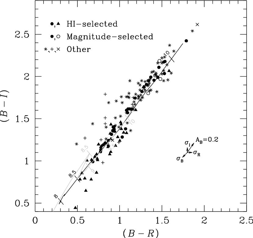
Figure 6: Color–color plot of galaxies observed in $B$, $R$, and $I$ in this study. The magnitudes are determined within the extinction-corrected $\mu_{B}=25$ mag arcsec^-2 isophote. Filled circles and triangles are HI-selected sources; open and filled circles are magnitude-selected. At the right of the figure are shown the effect of the estimated 1$\sigma$ errors in each magnitude and of an internal extinction of $A_{B}=0.2$ mag. Data for HI-selected sources of Szomoru et al. (1994) are shown by $+$ symbols and data from the diameter-limited sample of de Jong & van der Kruit (1994) by $\ast$ symbols. Black and gray curves show a stellar population synthesis model of the color evolution of populations with solar and 1/50th solar metallicity respectively, with log(age in years) marked at half decade intervals.

The dispersion about a best-fit linear relationship of $(B-I)=1.36\times(B-R)+0.03$ is only 0.097 mag. If we assume the $B$, $R$, and $I$ magnitudes each have the same intrinsic dispersion, we would recover this relationship if the true relationship was $(B-I)=1.41\times(B-R)-0.03$ and a 1–$\sigma$ uncertainty in each magnitude of 0.056. This assumes no intrinsic scatter in the relationship, so the actual uncertainty is presumably smaller.

This figure also shows the color data for HI-selected galaxies studied by Szomoru et al. (1994), and the data from de Jong & van der Kruit (1994) for a complete, diameter-limited sample of galaxies ranging from type Sa to Irr. Their quoted errors appear to account for the scatter relative to our empirical relationship, although there is a slight indication that the $(B-I)$ values might be slightly redder than ours toward the blue end of the curve. None of their sources reach the extreme blue colors of our ten bluest objects, which have mean colors of $(B-R)=0.63$ and $(R-I)=0.26$.

3.3 Surface Brightness Structure

In the last four columns of Table 4 we describe the surface brightness structure of our objects. Column (15) gives the central surface brightness as measured in the central brightest pixel of the $B$-band image, corrected for extinction. The remaining columns of the table describe our best fits to the $B$-band surface brightness distribution with combinations of disk and bulge components.

The fits are based on elliptical isophotal fits to the surface brightness data (corrected for extinction and inclination). As already noted, the inclination correction is only appropriate if the stars are in a thin disk, which may be inappropriate for dwarf, irregular, and elliptical systems as well as the central bulges of disk systems. We could have attempted to handle some galaxies and some regions within galaxies differently, but this would have introduced a degree of arbitrariness we preferred to avoid. In any case, we made fits with and without inclination corrections, and while individual galaxies’ parameters were altered slightly, the types of fits and overall sample behavior were unaffected.

We initially attempted to fit the radial profiles by a traditional combination of an exponential disk with an $r^{(}1/4)$-law bulge, exemplified by source #67 in Fig. 7. As has been noted by Andredakis & Sanders (1994), for many late-type galaxies this does not yield as good a fit as using an exponential fit to the bulge. An $r^{1/4}$-law fit is forced to have a shallow peak to match the central light distribution in these galaxies, which in turn forces the outer portions of the fit to be too high. Source #62 in Fig. 7 is an example of a source which is better fit by an exponential bulge. In column (16) of Table 4 we list what fraction of the total light from the galaxy is contributed by the bulge component ($f_{B}$). This fraction was fairly consistent whichever type of bulge was fit to a particular galaxy. The value is marked by a $q$ to indicate a “quarter-law” ($r^{1/4}$) fit or by an $e$ to indicate an exponential fit. The scale length and surface brightness parameters of the bulge fits depended sensitively on our handling of the axis-ratio corrections; we do not list them here.

Figure 7: Radial $B$-band profiles of four of the HI-selected galaxies, illustrating various kinds of fits. Source #67 has a traditional combination of an exponential disk (dotted line) and $r^{1/4}$-law bulge, while source #62 has an exponential bulge (bulges shown by dashed line). Source #43 shows only an exponential disk, and source #1 has an exponential disk that steepens in the outer portion (long dashed line).

The disk region was fit by an exponential law:

$$\mu(r)=\mu_{d}+2.5{r\over r_{d}}\log e\ ,$$

where $\mu_{d}$ is the projected central surface brightness of the disk component, and $r_{d}$ is its scale length. This was performed iteratively with the $r^{1/4}$ or exponential bulge to yield a least squares best fit. The exponential disk parameters are listed in columns (17) and (18) of Table 4.

Ten galaxies were best fit by an $r^{1/4}$–law profile without an exponential disk, and almost all of these had “bumps” in their radial profiles. These bumps also tended to occur in regions where there were significant changes in the estimated axis ratio, and tended to be weaker in the inclination-corrected fits, suggesting they may be part of a disk component that our simple distributions could not model.

For almost half (34 of 75) of the HI-selected galaxies no bulge component is evident. This is illustrated by source #43 in Fig. 7. As can be seen from the values of $f_{B}$ in Table 4, we fit bulges which contributed as little as 1% of the total galaxy light, and these are fairly obvious. We therefore assume any bulge component in the “bulgeless” galaxies contributes $\lesssim$1%. Note that even though there is no bulge component, $\mu_{d}$ does not necessarily match the observed central surface brightness. This is because $\mu_{d}$ is fit to the inclination-corrected surface brightnesses, which can make it fainter than the observed value, and it is corrected for seeing, which can make it brighter.

Finally, we noticed that the surface brightness profiles appear to turn over to a steeper slope in several galaxies. This behavior, illustrated by source #1 in the figure, cannot be modeled by a sum of components, and instead represents a cut-off to the fits found interior to it. The portion of the total light coming from these steep outer exponential disks ranged from 10 to 40% of the whole galaxy. This behavior occurs occasionally in all the various combinations of bulge and disk fits to the profiles, and has been noted in other studies of LSB galaxies (Davies, Phillipps, & Disney 1990; Rönnback & Bergvall 1994; Vennik et al. 1996). For the purpose of estimating the bulge fraction in column (13), we count this exponential cut-off region as part of the disk contribution. One possibility is that this change in scale length might be caused by imperfect modeling of changes in the galaxy inclination or position angle. For those interested in following up on these systems, we list their cut-off parameters in Table 5. The fraction of the total light in the cut-off region $f_{x}$ is listed in column (2), the surface brightness $\mu_{x}$ where the turnover begins in column (3), and the scale length $r_{x}$ of the exponential cut-off in column (4).

4 Relationships between Galaxy Properties

The sample of objects found in this HI survey has a number of properties that distinguish it from an optically-selected sample. We highlight the properties of our sample here, and discuss general implications for the overall galaxy population.

4.1 Spatial Distribution

We note first that most of the objects we detected at very low redshifts were not previously detected, suggesting that that the census of objects at very low redshifts is far from complete. Out to $cz_{hel}=3000$ km s^-1, nine sources were found in the HI survey, none of which is in the magnitude limited surveys, and only three of which were found by diameter-limited surveys. Even within 1000 km s^-1, the HI survey reveals three objects not found in any other surveys. These are dwarf galaxies, but their numbers over such a small area and with such a limited depth of sensitivity implies a very large number density. The implications of these sources for the galaxy mass function are discussed by Schneider et al. (1998).

The positions of the Arecibo Slice galaxies relative to the large scale structure in the vicinity is shown in Fig. 8. Positions of RC3 (de Vaucouleurs et al. 1991) galaxies within 10^∘ of the slice (but excluding the slice itself) are plotted in gray. All of the galaxies, whether they are from our optically-faint subset or they are LSB objects, basically follow the same large scale structure traced out by the optical surveys, as has been noted previously (for example, Mo, McGaugh, & Bothun 1994; Thuan, Gott, & Schneider 1987).

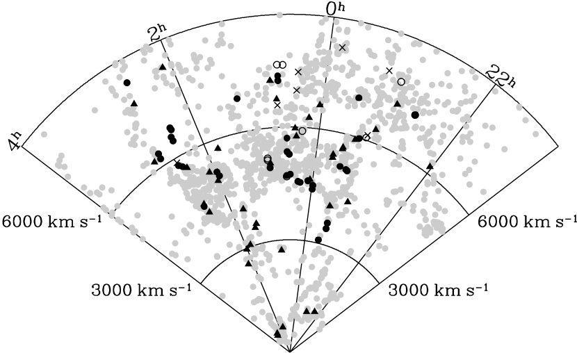
Figure 8: Location of slice objects relative to the local large scale structure. Redshifts of sources are plotted as a function of R.A. Locations of RC3 galaxies north and south of the search region between $13^{\circ}<\delta<34^{\circ}$ are shown in gray. Objects detected in the slice survey are shown in black: filled circles and triangles are HI-selected sources; open and filled circles are magnitude-selected; $\times$’s are neither.

One cautionary note should be made before drawing inferences about populations in voids: this is a redshift-space diagram, and patterns of large scale flow around the Pisces-Perseus supercluster and the Local supercluster may create the appearance of voids where none exist (see Praton & Schneider 1994). For example, if the “bubble” in the center of our slice diagram is delineated by velocity caustics of galaxies flowing toward infall centers in the supercluster, then this region should appear empty in redshift-space for any population of objects because it represents only a small volume of real space.

4.2 Optical versus HI Selection

In order to understand the selection effects of different survey approaches, we plot in Fig. 9 various measured quantities as a function of the galaxy redshift. We again use the notation from Fig. 4, in which circles represent magnitude-selected sources and solid symbols HI-selected sources. Panel (a) shows that the galaxies from the magnitude-limited catalogs are brighter than 16 mag (marked by a dotted line) with only a few exceptions. This is as expected, although since these catalogs implicitly depend on surface brightness and morphological identification, there is at least the potential for some LSB galaxies with brighter total magnitude to be missed. We find none such in our HI-selected sample.

Figure 9: Observed properties of sample galaxies as a function of redshift. Filled circles and triangles are HI-selected sources; open and filled circles are magnitude-selected; $\times$’s are neither. Panels (a) and (b) show the observed (uncorrected) Holmberg blue magnitude and major diameter. Panel (c) shows the HI flux, and panel (d) gives the ratio, in solar units, of the blue luminosity to the HI mass. Lines indicate the approximate break between the optically-bright and -faint halves of the HI-selected sample.

In panel (b) we plot the galaxies’ Holmberg diameters. Again, the sample separates fairly neatly into optically-bright and -faint halves at around 1 arcmin. This accords with the strong overlap between the magnitude- and diameter-limited samples noted in §3.1. The degree of correlation between the optical flux and surface area is also shown by the relatively small scatter in the ratio of these quantities: the standard deviation of log(optical flux/area) is 0.28 among the HI-selected objects.

In panel (c) we show the HI fluxes of the sources. It is clear that we cannot draw a simple boundary dividing optically-bright and -faint sources in this plot. The standard deviation of log(optical flux/HI flux) is 0.43. This lack of correlation of the HI and optical properties is somewhat surprising in light of previous work showing that the HI content is well-correlated with the optical disk size, independent of morphological type (Haynes & Giovanelli 1984). A large part of the difference comes from the non-HI-selected sources which have a much lower mean HI surface density (measured by the total HI flux and the Holmberg radius), but there is much more intermingling of optically-bright and -faint sources than is seen in Fig. 9(b). If we restrict ourselves to the magnitude-limited subset of our HI-selected sample, the average HI surface density properties are similar to the Haynes & Giovanelli sample, as might be expected since they were observing optically-selected objects.

Finally, panel (d) shows the ratio of total $I$-band luminosity to total HI mass. Since both depend on $d^{2}$, we can find the distance-independent “star-to-gas” ratio of the two:

$${L_{I}\over M_{HI}}=4.24\times 10^{4}10^{-0.4(B_{T}^{0}-4.02)}/\int S\,dv\ ,$$

where the result is in solar units of mass and luminosity for an absolute magnitude of the Sun at $I$ of 4.02.

We select the $I$-band luminosity because it is much less dependent on stellar evolution than $B$-band. McGaugh & de Blok (1997) suggest that the mass-to-light conversion from $I$-band luminosities to total stellar masses is nearly uniform at a factor of 1.2 for a wide range of stellar population ages. We find similar values based on a variety of models of the star-formation history using the population synthesis models of Bruzual & Charlot (1993), although for the very youngest blue populations the stellar mass-to-light ratio may be much less than 1, and for extremely old populations (which have had no star formation after an initial burst) the ratio may be as large as 3–4. To determine the total gas mass, the HI mass must be corrected by a similar factor of 1.3 to account for primordial helium. In addition there is potentially a large contribution from molecular gas, although this is probably larger in the same redder, earlier-type galaxies in which the stellar mass correction is larger (Young & Knezek 1989). All things considered, the $L_{I}/M_{HI}$ value is probably a reasonable estimator of the true star-to-gas mass ratio.

The optically-bright sources divide fairly cleanly from the rest of the sources near a star-to-gas mass ratio of 1, indicating that there is a physical basis for the distinction between the optically-bright and -faint subsets of our HI sample than just their apparent magnitudes. Only 2 of the optically-bright HI sources have a star-to-gas ratio $<0.8$, and only 3 of the optically-faint HI sources have a star-to-gas ratio $>1.2$. Thus the magnitude-limited sources are “star-dominated,” with an average of $\sim 2.7\times$ more mass in stars than gas, reaching $>10\times$ among the non-HI-selected objects. The optically-faint HI objects are “gas-dominated,” with an average gas mass $\sim 2.5\times$ the stellar mass, and reaching a factor $>10$ in the most most extreme case.

Some of the gas-dominated sources were found by other types of surveys, but these are not our most extreme objects. Seven of them were identified in diameter-limited and LSB surveys, but the most extreme of these (curiously a UGC object, #45) has only the sixth smallest star-to-gas ratio overall. These 7 diameter-selected sources have fairly typical blue colors of the gas-dominated subset. The bluest of these #2 (LSB F533-01) is only 12th bluest object overall. These surveys do identify several of our lowest surface brightness objects, including those with the 3rd, 5th, and 6th faintest $\mu_{1/2}$ values.

Four of the optically-faint HI sources were identified in UV-excess and emission-line surveys. These objects have colors and surface brightnesses that are typical of the star-dominated subset, and $L_{I}/M_{HI}$ ratios that are borderline between the subsets. The only significant exception is #57, which has the 11th bluest $(B-R)$ color. This object is also the only gas-dominated source detected by IRAS. It appears to be interacting with a small neighbor as we discussed in §3.1, and its nucleus appears to be off center. Two other of these sources also have off-center nuclei, suggesting that interactions may be responsible for these sources being detected by alternative methods.

4.3 Biases in Optical versus HI Selection

The HI selection criteria diverge in a fundamental way from the optical selection criteria. Consider that the HI selection identifies about twice as many sources as are found down to a magnitude limit of 16 in the same volume. To double the size of a magnitude-limited sample within this volume would require increasing the magnitude limit by only about 0.8 mag. However, to catch all but the faintest HI source based on their starlight would require a survey 4 mag deeper, with about 30 times more sources in this volume. Further, since optical surveys do not distinguish sources by redshift, a magnitude-limited survey 4 mag deeper would have about 250$\times$ more sources that would have to be identified and measured in order to detect these HI-selected sources.

The converse would of course be true if we were using HI to track down optically bright galaxies. For example, most E and S0 galaxies would be much easier to identify by optical search techniques than to find them by the signal from the small amount of HI present. The implications of this obvious difference are a little more subtle, however.

If we were to define the HI properties of S0 galaxies from our HI-selected sample, we might erroneously conclude that their HI content is fairly large. The four S0 galaxies in our HI-selected sample have an HI emission about $25\%$ of their $B$-band emission (in solar units). The one identified S0 galaxy among the non-HI-selected objects has an upper limit of $<1\%$. Obviously, HI-rich S0 galaxies are over-represented when we select sources by their HI content. The reverse will also occur: the HI content of galaxies will be underestimated in optically-selected samples.

This is akin to a Malmquist bias—flux-limited samples favor sources with intrinsically larger luminosities. When comparing two properties like HI and optical emission, this has the effect of exaggerating the level of the property being used for the flux limit. The weaker the correlation between the quantities, the bigger the effect, so it is important to determine HI properties of galaxies from HI-selected samples.

4.4 Surface Brightness Behavior

The distribution of light varies quite strongly between the star-dominated and gas-dominated galaxies. We quantify this here by a closer examination of the radial surface brightness distributions. We shall also show that these effects do not simply result from differences due to galaxy mass or luminosity, but appear to indicate a genuine difference in character of HI-selected galaxies.

The radial fits to the galaxies’ light distributions show a wide range of properties that vary from no bulge component to no disk component, and exponential or $r^{1/4}$-law bulges (see §3.3). These properties correlate strongly with the HI characteristics of the galaxies. Dividing the galaxies into the optically-faint and optically-bright halves of our HI-selected sample and the other magnitude-selected objects, we list the number of galaxies having no bulge, or an exponential or $r^{1/4}$-law bulge below:

	pure disk	exp bulge	$r^{1/4}$-law bulge
Optically-faint	29	11	00
Optically-bright	05	19	11
Non-HI-selected	01	02	04

The optically-faint subsample is much more likely to have no bulge at all, and none have $r^{1/4}$-law bulges. The situation is nearly reversed with the non-HI-selected galaxies, and the other magnitude-selected sources have a similarly strong tendency to have bulges, but more likely for these to be exponential bulges. Thus 73% of optically-faint sources have pure disks, while 86% of magnitude-limited sources have a bulge component.

Another way of quantifying this comparison is to look at the fraction of light contained in the bulge component for the different subsets. For the 40 optically-faint HI sources the bulge contributes on average 5% of the light, but for the 35 optically-bright HI sources the contribution rises to 29%, and for the 7 magnitude-selected, but non-HI-selected sources the contribution climbs to 61%.

Since the fraction of light from the bulge is correlated with galaxies’ mass and luminosity, it should be asked whether the trends seen here simply reflect that the HI sources tend to have lower luminosities and masses. We have avoided bringing in distance-dependent quantities in this paper, but to clarify this point we consider objects within a narrower range of mass and luminosity in which the different sample subsets are well-represented. For the sources with dynamical masses estimated between $10^{10}$ and $10^{11}M\sun$, the bulge fractions are 6%, 29%, and 50% for the optically-faint, optically-bright, and non-HI-selected subsets respectively. Very similar numbers are found when selecting sources with HI masses between $10^{9}$ and $10^{10}M\sun$: the corresponding bulge fractions are 9%, 20%, and 67%.

What remains clear even when comparing mass and luminosity ranges in which the subsamples fully overlap is that the HI-selected sources have distinctly different disk/bulge properties than the optically-selected sources. Still, this difference might be attributed to morphological-type variations, but these are often subjective and vague. What would be preferable is some type of quantitative, distance-independent measure of galaxy properties that relates relative stellar and gas content of galaxies like the $L_{I}/M_{HI}$ ratio, which we examine next.

Figure 10: Ratio of $I$-band and HI emission plotted against several different quantities: (a) the disk central surface brightness; (b) the mean Filled circles and triangles are HI-selected sources; open and filled circles are magnitude-selected; $\times$’s are neither. $I$-band surface brightness; (c) the $(B-R)$ color.

4.5 Surface Brightness Correlations

McGaugh & de Blok (1997) have noted a strong correlation between the star-to-gas mass ratio and the disk central surface brightness. Our HI-selected sample shows a weaker correlation between these quantities, as shown in Fig. 10(a). We find the correlation coefficient $\rho=0.65$ between $L_{I}/M_{HI}$ and $\mu_{d}$, and only $\rho=0.49$ using the $B$-band data, which is less than the value of $\rho=0.73$ found by McGaugh & de Blok. We suspect the stronger correlation they found may be because they collected data from different sources over the different surface-brightness ranges. As they note, they used data for optically bright galaxies and combined it with LSB objects selected to complement that data set. This enhances the number of uncataloged LSB objects, which generally have higher relative gas content, but it may also miss the occasional magnitude-limited source with a faint disk or HI-selected source with a relatively bright disk, as are seen in our scatter plot.

We find a much stronger correlation between $L_{I}/M_{HI}$ and the overall galaxy surface brightness than with the disk component alone. McGaugh (1996) has pointed out the problems with defining a surface brightness using total magnitudes and angular areas, the basic problem being that the isophotal radius measures the light over an essentially arbitrary portion of a galaxy’s disk. However, a robust measure of the average surface brightness can be made within the half-light or effective radius:

$$\mu_{1/2}=I_{tot}+2.5\log(2\pi r_{1/2}^{2})\ .$$

This relationship, shown in Fig. 10(b), has $\rho=0.82$, which is stronger than any of the correlations found by McGaugh & de Blok (1997).

Because our $I$–band data did not have very good seeing, we have used the $B$–band effective radii, but this should make little difference. The correlation is only slightly diminished if we use $B$-band values instead ($\rho=0.76$), or use mixes of $B$– and $I$–band data for the surface brightness or star-to-gas ratio ($\rho=0.81$ and 0.70). The correlation is noticeably weaker for the magnitude-selected set of galaxies alone, although still significant: $\rho=0.62$ using $I$ values; $\rho=0.54$ using $B$. This reduced correlation is like the effect McGaugh & de Blok found when they excluded LSB galaxies from their sample, but the values we find for our magnitude-limited sample is still comparable to the strongest correlations they found for their full sample. We therefore believe this measure of surface brightness is a more powerful predictor of the relative gas and stellar content of galaxies.

4.6 Color Correlations

Another correlation that has been noted previously (Schneider 1996; McGaugh & de Blok 1997) is between the galaxy color and the star-to-gas ratio. Again, this is in the sense one might expect, that galaxies with apparently more conversion of gas into stars appear redder. The correlation we find is stronger than that noted by McGaugh & de Blok, although not quite as strong as the correlation with surface brightness. The data are shown in Fig. 10(c), and correlation coefficient between the $(B-R)$ color and $\log(L_{I}/M_{HI})$ is $\rho=0.72$ ($\rho=0.71$ for the magnitude-selected objects alone).

The correlation substantially weakens when using the blue luminosity in the star-to-gas ratio. It drops to $\rho=0.51$. We suspect that this difference primarily reflects that $I$-band is the better measure of the galaxies’ stellar content. These correlations all appear to be consistent with a paradigm in which the galaxies evolve as gas is consumed to make stars. This is clearly an oversimplification since the objects we are examining span a wide range of masses and sizes, with the smallest objects showing the least gas consumption. However this paradigm may be appropriate for a scenario in which larger galaxies form from the accretion of smaller galaxies.

Turning back to Fig. 6, note the color evolution curves marked on the plot. These are based on the population synthesis code of Bruzual & Charlot (1993, 1998) for a population of stars that has a single burst of star formation. The log of the age of the population in years after the burst is marked along each curve, which show results for two different metallicities: solar (black line) and 1/50th solar (gray line).

Both curves closely follow the empirical relationship between $(B-R)$ and $(B-I)$ found earlier. Since the evolutionary tracks are nearly linear in the color-color diagram, any pattern of star-forming histories should also lie along this line. The bluest objects have colors comparable to a starburst $<10^{9}$ yr ago. Combinations of such a starburst with a pre-existing population would yield redder colors, suggesting an even younger starburst, but it should be kept in mind that a starburst only $10^{8}$ yr old can generate many times more light per unit mass than a population $>10^{9}$ yr old. Thus we do not suggest using the colors as a simple age indicator so much as a relative indication of the amount of star formation that has taken place recently.

5 Summary

We have presented data from a large, sensitive search for extragalactic sources in the 21 cm line of neutral hydrogen, which has detected some of the lowest mass HI sources found in a blind survey to date. The survey was made with the Arecibo radio telescope and covers about 55 deg² out to over 100 Mpc. The survey region is in the general vicinity of the Pisces-Perseus supercluster, crossing through the supergalactic plane, and it is all at high enough Galactic latitudes ($|b|>25^{\circ}$) that the extinction is moderate ($A_{B}\lesssim 1$). We have obtained $BRI$ photometry for nearly the entire sample, and examined other objects found within the same volume. In total, 75 objects were found by the HI survey, 39% of these being previously unidentified objects.

Cross-references to other catalogs allow us to examine selection criteria of the different survey techniques and how they relate to physical characteristics of the galaxies. In general, we find that the optical survey techniques tend to collect strongly nucleated, high surface brightness galaxies. The newly detected HI sources appear to represent a population of faint blue dwarfs, often with substantially larger gas than stellar masses.

There are several interesting aspects of the HI-selected sample:

(1) At low redshifts, where the HI survey is sensitive to low mass objects, we detect three new objects at $cz<1000$km s^-1, one of which (#75) has no clear optical counterpart (although it is too near a bright star to rule out a very low surface brightness counterpart). Out to $cz<3000$km s^-1, 6 of 9 sources are new detections.

(2) The new detections in this survey are, not-surprisingly, HI-bright relative to the objects found in previous optical surveys. They are also gas-dominated objects based on estimations of their total stellar mass from their $I$-band photometry. Thirteen objects, spanning a wide range of masses, have a star-to-gas mass ratio less than 1/3 not including source #75 whose optical counterpart has not been identified. Only 3 of these objects were found previously in diameter-limited searches for LSB sources.

(3) The distribution of light in the new detections is systematically different from the optically-selected galaxies. They are much less likely to have any bulge component, and this tendency is not just a result of selecting lower-mass objects (§4.2).

(4) The galaxies show a wide range of colors, but follow color-color tracks of population synthesis models of stellar evolution closely. The new HI-detected sources tend to be bluer on average, and our bluest ten objects lie at younger ages along the evolution track than any of the objects drawn from either the complete diameter-limited sample of galaxies of de Jong & van der Kruit (1994) or the HI-selected sample of Szomoru et al. (1994).

(5) We find strong correlations between the galaxy star-to-gas mass ratio and the mean surface brightness and color of these galaxies. The strongest correlation is found between the star-to-gas mass ratio and the mean surface brightness within the half-light radius. VLA observations of our lowest surface brightness source (#14) indicate that its surface density of HI is well below the threshold for star formation.

Table 1: HI Observations in Arecibo Slice.

			$cz_{hel}$	$w_{50}$	$w_{20}$		$\int S_{cen}\,dv$	$\int S_{tot}\,dv$	$\int S_{det}\,dv$	$w_{det}$	offset
No.	$\alpha$ (1950) $\delta$		(km s-1)	(km s-1)	(km s-1)	$N_{h}$	(Jy km s-1)	(Jy km s-1)	(Jy km s-1)	(km s-1)	(arcmin)
(1)	(2)		(3)	(4)	(5)	(6)	(7)	(8)	(9)	(10)	(11)
1	22 02 07.9	+23 04 13	6206	081	150	3	1.36	1.66	0.80	116	1.7
2	22 25 44.5	+23 07 23	1278	062	082	1	2.66	3.53	1.73	076	0.8
3	22 38 58.2	+23 07 07	7154	087	130	1	4.14	4.78	3.21	142	0.5
4	22 56 31.2	+23 44 15	7189	039	125	3	0.83	1.19	0.54	161	1.7
5	23 01 13.7	+23 25 07	1155	096	111	2	2.75	2.85	0.58	106	1.7
6	23 05 37.3	+22 59 16	6336	031	050	1	1.46	1.62	1.20	045	0.8
7	23 06 06.9	+23 21 49	4270	130	149	2	2.76	3.38	1.90	139	1.6
8	23 18 22.0	+23 32 22	5961	578	612	2	2.38	3.31	1.96	514	1.3
9	23 20 10.2	+23 06 03	5042	118	174	3	1.38	2.27	0.72	131	1.6
10	23 21 47.3	+23 33 52	5895	122	154	2	1.93	2.10	0.76	140	2.1
11	23 22 04.2	+23 42 49	5063	264	283	2	2.39	4.15	1.50	274	1.8
12	23 25 12.2	+23 18 51	3403	095	166	1	6.78	8.86	1.95	200	2.2
13	23 25 35.7	+23 15 29	3556	269	294	2	9.43	13.800	4.30	402	1.7
14	23 29 06.3	+23 45 42	4009	059	088	1	0.76	0.96	0.65	132	2.0
15	23 29 31.2	+23 17 01	6989	239	249	2	2.27	2.92	1.47	267	0.9
16	23 29 58.8	+23 39 35	5095	408	423	2	2.55	3.44	1.66	431	1.6
17	23 31 57.3	+23 38 48	5603	164	189	2	0.92	1.68	0.87	166	0.1
18	23 32 15.2	+23 41 44	5558	111	135	1	2.41	2.69	0.87	138	2.1
19	23 33 21.0	+23 20 55	3054	188	208	2	4.06	5.46	3.14	209	0.8
20	$\sim$23 40 43.5	+23 13 51	5355	331	344	2	2.46	3.01	2.37	344	1.2
21	23 40 46.6	+23 14 08	5271	043	063	1	0.51	0.66	0.55	063	0.4
22	$\sim$23 59 05.0	+23 12 46	$\sim$4325	$\sim$590	—	2	$\sim$7.14	$\sim$9.45	12.360	623	1.6
23	$\sim$23 59 05.0	+23 12 46	$\sim$4430	$\sim$540	—	2	$\sim$4.76	$\sim$6.30	12.410	623	1.6
24	00 02 32.8	+23 41 37	6573	133	178	2	2.34	2.72	1.28	196	2.1
25	00 03 49.1	+23 30 59	4574	197	259	2	3.52	4.26	1.76	221	1.3
26	00 06 20.1	+23 32 13	4528	152	192	3	3.83	4.12	1.78	235	1.6
27	00 11 23.6	+23 41 37	6201	138	154	2	1.29	1.38	1.14	161	0.7
28	00 16 24.3	+23 11 49	4459	221	234	2	5.02	5.59	3.28	243	1.2
29	00 19 27.7	+23 27 32	4479	237	253	2	4.03	4.80	3.31	258	1.0
30	00 23 22.8	+23 39 09	5679	190	198	2	1.10	1.08	0.60	141	1.8
31	00 24 51.0	+23 26 53	5884	188	259	2	0.93	1.23	0.43	123	1.6
32	00 29 54.7	+23 06 57	4658	213	230	2	3.58	4.56	3.31	249	1.3
33	00 30 59.3	+23 07 21	5190	268	280	2	2.70	2.64	2.12	271	1.2
34	00 33 19.5	+23 45 35	5614	222	238	2	1.33	1.60	0.81	101	1.7
35	00 33 25.1	+23 40 40	5252	524	544	2	3.15	3.08	1.03	525	1.9
36	00 34 15.7	+23 43 01	4618	549	625	2	6.22	8.30	5.32	657	1.1
37	$\sim$00 40 15.5	+23 13 08	7274	342	368	2	2.00	2.10	1.66	174	1.5
38	$\sim$00 40 15.5	+23 13 08	7148	114	166	3	1.15	1.15	0.93	098	1.5
39	00 42 12.8	+23 32 09	6650	061	074	3	0.60	0.59	0.53	107	0.9
40	$\sim$00 46 54.4	+23 47 37	7157	138	177	2	0.81	1.39	0.63	141	1.9
41	00 49 15.1	+23 12 34	2622	066	080	2	0.71	0.91	0.54	120	1.9
42	00 53 36.6	+23 46 55	4962	047	055	1	0.44	0.44	0.32	053	1.3
43	00 54 39.2	+23 36 50	4834	171	203	3	3.67	4.41	1.95	213	1.7
44	01 17 15.9	+23 42 06	6777	224	246	2	3.18	4.01	1.52	408	1.9
45	01 28 36.6	+23 41 45	3415	063	098	1	4.69	6.66	2.68	090	1.6
46	01 32 24.1	+23 45 22	3316	115	144	2	5.03	7.57	2.10	131	2.1
47	01 33 51.3	+23 33 56	0563	051	066	1	1.16	1.76	0.56	091	1.6
48	01 42 21.3	+23 31 15	3874	044	058	1	0.54	0.86	0.47	057	1.4
49	01 47 54.7	+23 09 17	5614	332	411	2	1.55	2.09	0.72	165	2.3
50	01 51 05.7	+23 39 58	2914	118	146	2	1.69	2.03	1.11	165	1.3
51	01 57 07.1	+23 24 23	4919	124	158	3	4.93	5.46	2.98	180	0.6
52	01 57 57.0	+23 30 46	5029	121	139	2	1.41	1.79	0.75	111	1.8
53	01 58 14.8	+23 10 39	5041	171	210	3	2.04	2.49	1.38	180	1.4
54	02 00 32.3	+23 31 05	2832	122	143	2	1.74	2.27	1.25	118	1.4
55	02 00 55.8	+23 47 08	4812	252	294	2	1.79	2.42	0.30	065	2.1
56	02 06 17.3	+23 36 19	5105	064	082	1	1.26	1.54	0.96	089	1.0
57	02 06 19.8	+23 00 58	8162	169	251	3	2.59	3.11	1.37	160	0.7
58	02 10 47.7	+23 00 49	2452	054	072	1	0.34	0.39	0.19	039	0.5
59	$\sim$02 22 20.6	+23 37 08	6574	069	104	1	1.53	2.03	0.86	206	1.7
60	$\sim$02 22 31.5	+23 36 15	6631	180	213	2	1.78	2.06	1.40	203	1.0
61	02 25 29.5	+22 59 26	6399	398	436	2	4.19	5.88	3.28	429	0.9
62	02 25 48.9	+23 34 09	6287	296	315	2	2.30	2.91	1.63	156	1.2
63	02 26 30.7	+23 44 58	5484	247	267	2	1.49	1.85	1.24	265	1.0
64	02 29 34.0	+23 25 35	4159	120	142	2	1.40	1.37	1.27	148	0.8
65	02 30 02.8	+23 06 02	5563	250	266	2	5.31	5.83	4.44	277	1.5
66	02 30 39.6	+23 15 42	4414	160	176	2	1.40	1.89	1.08	174	1.6
67	02 31 52.7	+23 11 43	4360	606	633	2	9.18	12.480	6.44	633	1.3
68	02 33 18.1	+23 40 54	5649	246	278	2	7.47	9.29	4.93	265	1.5
69	02 34 37.0	+23 05 13	8239	319	368	2	2.70	2.85	0.61	273	1.4
70	02 38 25.3	+23 03 07	7661	174	189	3	0.91	1.34	0.75	199	1.9
71	02 44 03.7	+23 23 16	6196	345	386	2	2.68	3.67	1.01	417	2.0
72	02 45 00.9	+23 11 56	6054	319	332	2	4.07	4.32	1.82	465	2.2
73	02 45 46.7	+23 03 45	0469	030	053	1	0.97	1.07	0.31	034	0.4
74	02 51 49.9	+23 10 41	6071	116	140	2	1.63	1.68	1.16	140	1.1
75	02 54 40.1	+23 35 13	0411	031	051	1	0.49	0.64	0.23	061	1.0
Non-HI-Selected Sources
76	22 38 50.3	+23 08 18	7148	—	—	—	$confused$	—	—	—	1.9
77	23 00 42.9	+23 29 22	7775	156	161	2	0.47	—	$\sim$0.14	$\sim$161	2.1
78	23 11 20.5	+23 32 53	6122	108	128	3	0.17	—	$\sim$0.07	$\sim$128	1.9
79	23 12 01.3	+23 24 47	6048	—	—	—	$<$0.10	—	—	—	1.8
80	23 12 24.1	+23 00 39	7935	438	458	2	0.69	—	$\sim$0.32	$\sim$458	1.5
81	23 51 06.8	+23 21 16	8184	—	—	—	$<$0.18	—	—	—	1.6
82	00 17 14.3	+23 29 44	5829	389	405	2	0.65	—	0.58	356	1.8
83	00 23 20.3	+23 30 21	7389	206	228	2	1.61	2.34	0.60	242	1.9
84	00 24 15.4	+23 14 37	6896	090	106	—	$\sim$0.46	—	0.36	106	0.9
85	00 34 13.9	+23 42 34	4595	—	—	—	—	—	—	—	0.7
86	00 35 53.5	+23 20 13	7566	134	171	2	$confused$	—	$\sim$0.06	$\sim$171	1.7
87	00 40 24.0	+23 14 00	7571	359	390	2	1.10	1.56	0.80	390	1.4
88	00 41 41.3	+23 33 36	6493	0$\sim$37	0$\sim$69	—	$\sim$0.75	—	0.44	069	1.4
89	00 56 20.1	+23 34 58	5086	283	300	2	0.52	—	0.28	117	0.9
90	00 56 42.6	+23 42 35	5043	136	173	2	0.38	—	0.47	106	0.6
91	02 33 13.2	+23 36 40	5734	177	217	2	0.86	1.53	0.42	269	1.7

.6in offset dimensions No. $\alpha$ (1950) $\delta$ (arcmin) ${\int\displaystyle S_{V\!L\!A}\,dv\atop\ }\over{\ \atop\int\displaystyle S_{tot}\,dv}$ (arcmin) (1) (2) (3) (4) (5) 14 23 29 08.6 +23 45 27 0.58 1.15 $1.5\times 1.0$ 17 23 31 57.3 +23 37 54 0.90 0.36 $1.1\times 0.3$ 18 23 32 14.9 +23 41 37 0.14 0.91 $1.1\times 0.5$ 75 02 54 42.5 +23 35 11 0.55 0.63 $0.0\times 0.0$

Table 2: VLA HI Observations.

Table 3: Optical Counterparts to the HI-Selected Sample.

				Optical Catalog Cross-Identifications
			offset	Magnitude	Diameter	UV Excess/	IRAS FIR
No.	$\alpha$ (1950) $\delta$		(arcmin)	Limited	Limited	Emission Line	$60\mu$/	$100\mu$	Morphology
(1)	(2)		(3)	(4)	(5)	(6)	(7)		(8)
1	22 02 09.1	+23 04 38	0.5	—	—	—	—/	—	—
2	22 25 44.6	+23 07 07	0.3	—	LSBC F533–01	—	—/	—	Im
3	22 39 00.3	+23 06 50	0.6	IC 5243	UGC 12153	Ark 562/KUG	0.538/	$<$2.538	S? pec
4	22 56 33.6	+23 44 09	0.5	—	—	—	—/	—	—
5	23 01 14.8	+23 24 59	0.3	—	ESDO 535–04	—	—/	—	—
6	23 05 38.7	+22 59 24	0.3	—	—	—	—/	—	—
7	23 06 05.8	+23 21 38	0.3	—	—	—	—/	—	—
8	23 18 24.1	+23 32 00	0.6	CGCG 476–013	UGC 12533	—	—/	—	Sbc
9	23 20 08.0	+23 06 02	0.5	CGCG 476–023	—	—	—/	—	S
10	23 21 47.7	+23 34 08	0.3	—	—	—	—/	—	—
11	23 22 04.9	+23 42 42	0.2	CGCG 476–031	UGC 12583	—	—/	—	Scd
12	23 25 11.7	+23 18 49	0.1	NGC 7673	UGC 12607	Mrk 325/UCM/KUG	4.913/	6.893	(R′)SAc? pec
13	23 25 36.6	+23 15 22	0.2	NGC 7677	UGC 12610	Mrk 326/KUG	3.956/	5.915	SAB(rc)bc: pec
14	23 29 08.9	+23 45 38	0.6	—	—	—	—/	—	—
15	23 29 32.1	+23 16 55	0.2	CGCG 476–061	—	KUG	0.301/	$<$1.111	S?
16	23 29 59.7	+23 39 48	0.3	CGCG 476–064	UGC 12655	—	—/	—	S0
17	23 31 56.9	+23 37 39	1.2	—	—	—	—/	—	—
18	23 32 14.3	+23 41 42	0.2	—	—	—	—/	—	—
19	23 33 21.0	+23 20 32	0.4	NGC 7712	UGC 12694	KUG	0.656/	1.860	E?
20	23 40 43.0	+23 14 02	$\sim$0.2	—	FGC 2530	—	—/	—	Scd
21	23 40 46.0	+23 13 19	$\sim$0.8	—	—	—	—/	—	—
22	23 59 04.4	+23 12 22	$\sim$0.4	CGCG 477–040	UGC 12914	Kaz 240	6.128/	14.010	(R)S(r)cd: pec
23	23 59 08.0	+23 13 07	$\sim$0.8	CGCG 477–041	UGC 12915	—	6.128/	14.010	S? pec
24	00 02 30.7	+23 41 30	0.5	—	—	—	—/	—	—
25	00 03 48.4	+23 30 38	0.4	—	—	KUG	—/	—	S
26	00 06 19.7	+23 32 21	0.2	NGC 9	UGC 78	KUG/UCM	0.737/	1.527	Sb: pec
27	00 11 23.5	+23 41 28	0.2	—	—	KUG	—/	—	S
28	00 16 24.4	+23 12 02	0.2	CGCG 478–053	UGC 179	—	—/	—	Scd:
29	00 19 28.6	+23 27 33	0.2	CGCG 479–016	UGC 210	—	—/	—	Sb
30	00 23 20.0	+23 38 49	0.7	—	LSBC F473–01	—	—/	—	Im
31	00 24 50.8	+23 26 46	0.1	—	—	—	—/	—	—
32	00 29 54.7	+23 07 10	0.2	CGCG 479–037	UGC 321	—	—/	—	SBcd?
33	00 30 58.1	+23 07 20	0.3	CGCG 479–040	—	—	—/	—	S?
34	00 33 19.7	+23 45 43	0.1	MCG+04–02–032	UGC 354	—	—/	—	—
35	00 33 25.7	+23 40 58	0.3	NGC 160	UGC 356	—	—/	—	(R)SA0+ pec
36	00 34 13.5	+23 42 58	0.5	NGC 169	UGC 365	—	1.118/	3.668	SA(s)ab: pec
37	00 40 16.7	+23 12 50	$\sim$0.4	CGCG 479–061	—	UCM	0.783/	2.233	SB
38	00 40 18.7	+23 13 29	$\sim$0.8	NGC 228	UGC 458	—	—/	—	(R)SB(r)ab
39	00 42 12.6	+23 32 00	0.2	—	—	—	—/	—	—
40	00 47 02.8	+23 46 24	$\sim$2.3	—	—	—	—/	—	—
41	00 49 14.6	+23 12 35	0.1	—	—	—	—/	—	—
42	00 53 35.7	+23 46 59	0.2	—	—	—	—/	—	—
43	00 54 38.7	+23 37 10	0.3	CGCG 480–025	UGC 591	UCM	—/	—	S?
44	01 17 15.2	+23 42 09	0.2	MCG+04–04–003	—	—	—/	—	—
45	01 28 37.0	+23 41 48	0.1	—	UGC 1084	—	—/	—	Sm:
46	01 32 24.6	+23 45 06	0.3	—	—	—	—/	—	—
47	01 33 50.3	+23 33 37	0.4	—	—	—	—/	—	—
48	01 42 21.5	+23 31 08	0.1	—	—	—	—/	—	—
49	01 47 55.7	+23 09 08	0.3	—	—	UCM	—/	—	Sa
50	01 51 06.6	+23 40 02	0.2	—	—	—	—/	—	—
51	01 57 06.1	+23 24 07	0.3	NGC 776	UGC 1471	UCM	1.250/	3.099	SAB(rs)b
52	01 57 56.1	+23 30 56	0.3	—	—	—	—/	—	—
53	01 58 15.2	+23 10 37	0.1	CGCG 482–046	—	—	0.248/	0.818	S
54	02 00 32.4	+23 31 16	0.2	—	UGC 1538	—	—/	—	Im:
55	02 00 54.3	+23 47 18	0.4	—	—	—	—/	—	—
56	02 06 17.8	+23 36 23	0.1	—	—	—	—/	—	—
57	02 06 22.6	+23 00 56	0.7	—	—	UCM	0.602/	$<$1.369	Sc+
58	02 10 46.7	+23 01 29	0.7	—	—	—	—/	—	—
59	02 22 19.1	+23 37 36	$\sim$0.6	CGCG 483–034	—	—	—/	—	S?
60	02 22 31.0	+23 36 08	$\sim$0.2	CGCG 483–036	—	—	0.335/	$<$2.598	—
61	02 25 31.3	+22 59 29	0.4	CGCG 483–063	UGC 1938	—	0.293/	$<$1.688	Sbc
62	02 25 48.5	+23 34 24	0.3	CGCG 483–065	UGC 1950	—	0.360/	$<$1.631	S?
63	02 26 29.7	+23 44 54	0.2	—	—	—	—/	—	—
64	02 29 34.4	+23 25 58	0.4	—	—	—	—/	—	—
65	02 30 02.8	+23 06 27	0.4	CGCG 484–005	UGC 2020	—	—/	—	Scd:
66	02 30 37.9	+23 15 57	0.5	—	—	—	—/	—	—
67	02 31 51.5	+23 11 41	0.3	NGC 984	UGC 2059	—	—/	—	SA0+ pec
68	02 33 17.5	+23 40 55	0.1	CGCG 484–012	UGC 2079	—	0.513/	1.522	SAB(s)c
69	02 34 35.5	+23 05 02	0.4	CGCG 484–016	UGC 2104	—	0.386/	$<$1.408	Scd:
70	02 38 26.7	+23 03 18	0.4	—	—	—	—/	—	—
71	02 44 01.8	+23 23 10	0.4	CGCG 484–018	UGC 2248	—	0.847/	1.955	S0:
72	02 44 58.8	+23 11 49	0.5	CGCG 484–019	UGC 2267	—	—/	—	(R)SB(r)b
73	02 45 46.3	+23 03 58	0.2	—	—	—	—/	—	—
74	02 51 49.0	+23 10 28	0.3	—	LSBC F480-V03	—	—/	—	SBm
75	—		—	—	—	—	—/	—	—
Non-HI-Selected Sources
76	22 38 51.3	+23 08 47	—	IC 5242	UGC 12148	UCM	1.109/	$<$3.121	Sa
77	23 00 42.9	+23 29 22	—	CGCG 475–028	—	—	3.641/	5.515	—
78	23 11 20.5	+23 32 53	—	—	—	Mrk 317/KUG	0.667/	$<$2.799	S?
79	23 12 01.4	+23 24 45	—	NGC 7539	UGC 12443	—	—/	—	S0
80	23 12 25.0	+23 00 37	—	—	UGC 12449	—	—/	—	—
81	23 51 06.8	+23 21 16	—	—	—	UCM	—/	—	—
82	00 17 12.7	+23 29 42	—	IC 1540	UGC 186	—	—/	—	SBb
83	00 23 20.2	+23 30 29	0.1	—	—	—	—/	—	—
84	00 24 15.4	+23 14 37	—	—	—	HS	—/	—	—
85	00 34 13.9	+23 42 34	—	IC 1559	—	Mrk 341	1.118/	3.668	SAB pec:
86	00 35 53.6	+23 20 20	—	CGCG 479–049	—	Mrk 344	—/	—	E?
87	00 40 25.7	+23 14 08	—	NGC 229	—	—	—/	—	—
88	00 41 41.3	+23 33 36	—	—	—	HS	—/	—	—
89	00 56 19.9	+23 34 58	—	CGCG 480–028	UGC 612	—	0.339/	1.475	S?
90	00 56 42.5	+23 42 35	—	CGCG 480–029	—	—	—/	—	Sc
91	02 33 12.2	+23 36 48	0.3	—	—	—	0.214/	$<$0.942	—

Table 4: Optical Measurements of the HI-Selected Sample.

No.	$B_{25}$	$A_{B}$	$B^{0}_{25}$	$B^{0}_{T}$	$a_{25}$	$a_{H}$	$a_{1/2}$	$(b/a)$	$(b/a)_{H}$	P.A.	$(B$$-$$R)$	$(B$$-$$I)$	$(B$$-$$R)_{0}$	$\mu_{0}$	$f_{B}$	$\mu_{d}$	$r_{d}$
(1)	(2)	(3)	(4)	(5)	(6)	(7)	(8)	(9)	(10)	(11)	(12)	(13)	(14)	(15)	(16)	(17)	(18)
1	16.90	0.40	16.51	16.42	0.53′	0.67′	0.30′	0.80	0.80	129∘	0.86	1.16	0.75	22.05	—	22.45	07.6′′
2	18.07	0.23	18.05	16.94	0.39	0.91	0.58	0.69	0.82	062	0.73	0.86	0.81	23.72	—	23.85	09.8
3	14.66	0.26	14.41	14.39	0.74	0.89	0.30	0.86	0.89	011	0.69	$\sim$0.97	0.70	18.88	0.90q	—	—
4	16.97	0.65	16.54	16.29	0.60	0.85	0.34	0.21	0.27	142	1.08	1.33	1.15	21.61	—	22.36	05.9
5	17.54	0.56	17.11	16.65	0.47	0.83	0.38	0.48	0.53	133	0.78	1.17	0.79	22.37	—	22.81	06.5
6	19.95	0.83	19.17	17.51	0.21	0.69	0.50	0.44	0.92	078	0.73	1.08	0.89	22.85	0.06e	24.36	09.1
7	17.32	0.78	16.48	15.98	0.58	0.99	0.46	0.57	0.63	110	1.01	1.46	1.30	22.13	0.03e	22.91	08.0
8	15.67	0.38	15.67	15.24	0.86	1.67	0.61	0.20	0.17	018	1.47	$\sim$2.07	1.75	20.51	0.45q	23.05	11.9
9	16.10	0.27	15.84	15.74	0.52	0.75	0.22	0.84	0.84	179	0.78	1.13	1.00	21.00	—	20.86	03.8
10	18.27	0.20	18.50	17.81	0.27	0.58	0.29	0.57	0.61	124	0.88	1.08	0.92	22.81	—	23.23	05.0
11	16.18	0.20	16.40	16.04	0.74	1.19	0.51	0.18	0.18	053	—	—	—	21.61	0.03e	22.48	08.6
12	13.35	0.19	13.17	13.10	1.25	1.93	0.26	0.83	0.84	083	0.68	0.99	0.73	18.33	0.77e	22.70	14.8
13	14.18	0.18	14.08	13.96	1.48	2.03	0.50	0.54	0.60	037	1.12	1.62	1.43	19.91	0.40e	22.32	14.1
14	23.10	0.25	25.96	18.47	0.00	0.51	0.48	0.85	0.85	082	0.90	$\sim$1.28	0.91	25.02	—	25.06	09.6
15	15.71	0.28	15.44	15.23	0.53	0.95	0.22	0.81	0.68	088	1.10	1.62	1.29	20.05	0.44e	22.33	06.6
16	14.23	0.24	14.04	13.94	1.13	1.64	0.34	0.59	0.58	125	1.53	2.04	1.71	18.92	0.37e	21.40	09.5
17	17.11	0.32	16.88	16.77	0.38	0.53	0.20	0.43	0.61	049	0.74	1.01	0.78	21.22	—	21.50	03.6
18	18.00	0.32	17.80	17.44	0.33	0.56	0.25	0.62	0.72	133	0.60	0.65	0.68	22.39	—	22.60	04.0
19	14.26	0.23	14.03	13.99	0.97	1.25	0.42	0.81	0.94	104	1.14	1.61	1.61	20.06	0.60q	—	—
20	16.96	0.26	17.45	16.92	0.51	0.91	0.46	0.15	0.22	124	1.28	1.87	1.60	22.21	—	23.29	08.9
21	18.45	0.26	18.29	17.99	0.25	0.41	0.18	0.52	0.60	073	0.59	0.79	0.10	22.17	—	22.46	02.8
22	13.73	0.48	13.29	13.11	2.09	2.95	0.98	0.59	0.75	159	1.37	1.99	1.82	18.82	0.18q	22.17	20.0
23	14.71	0.48	14.30	14.17	1.36	1.89	0.58	0.27	0.27	134	1.29	1.88	1.02	20.10	0.03e	21.29	10.6
24	17.47	0.56	16.90	16.51	0.53	0.85	0.39	0.87	0.99	138	0.95	1.35	1.29	22.40	—	22.86	06.7
25	16.43	0.64	15.86	15.64	0.68	1.03	0.39	0.41	0.33	038	0.89	1.11	0.85	21.26	0.06e	22.04	06.7
26	15.01	0.40	14.67	14.54	0.86	1.33	0.34	0.49	0.44	156	0.87	1.18	0.85	20.02	0.64e	22.70	09.9
27	15.89	0.21	15.80	15.67	0.73	1.03	0.34	0.41	0.43	130	0.90	1.26	0.92	21.24	—	21.52	06.0
28	15.45	0.28	15.25	15.05	0.85	1.29	0.42	0.54	0.46	176	0.87	1.24	1.29	20.55	0.09q	21.72	07.8
29	15.35	0.18	15.24	15.13	0.92	1.19	0.46	0.42	0.42	018	1.03	1.28	1.23	20.70	0.26e	22.75	13.2
30	17.99	0.14	18.06	17.43	0.35	0.71	0.39	0.77	0.80	148	0.98	1.28	1.05	23.20	—	23.40	06.5
31	16.77	0.14	16.70	16.56	0.48	0.67	0.22	0.72	0.72	133	0.89	1.26	0.95	21.53	—	21.56	04.0
32	15.87	0.12	15.89	15.53	0.77	1.25	0.50	0.30	0.24	148	0.93	1.40	1.25	21.42	0.04e	22.42	08.9
33	15.68	0.12	15.65	15.53	0.73	0.97	0.42	0.47	0.45	128	1.09	1.57	1.35	21.35	0.08e	22.30	10.6
34	16.38	0.14	16.54	16.26	0.60	0.94	0.39	0.30	0.30	116	1.07	1.38	1.25	21.68	0.01e	22.35	06.5
35	13.59	0.13	13.55	13.42	1.89	2.57	0.84	0.51	0.55	045	1.45	1.99	1.55	18.83	0.82q	—	—
36	14.31	0.12	14.44	14.06	1.26	2.44	0.79	0.36	0.41	085	1.79	2.42	2.25	19.88	0.32e	23.05	20.5
37	15.86	0.16	15.86	15.56	0.65	1.05	0.42	0.40	0.45	051	1.54	2.18	1.94	21.00	0.05e	22.17	07.1
38	14.99	0.16	14.86	14.61	0.83	1.51	0.42	0.76	0.93	112	1.46	2.11	1.74	19.13	0.36q	22.27	10.1
39	18.32	0.15	18.57	18.15	0.24	0.44	0.20	0.74	0.87	135	0.66	0.78	0.64	22.61	—	22.68	03.3
40	16.56	0.17	16.50	16.33	0.39	0.67	0.16	0.79	0.80	069	1.58	2.07	1.43	20.49	0.61e	23.36	06.0
41	16.26	0.14	16.18	16.11	0.42	0.63	0.14	0.55	0.69	093	0.67	1.01	0.65	20.11	0.47e	21.70	03.8
42	17.86	0.23	18.32	17.56	0.32	0.65	0.39	0.49	0.88	153	1.00	1.24	0.91	23.07	—	23.47	06.1
43	15.42	0.20	15.27	15.19	0.75	1.05	0.34	0.61	0.68	155	0.77	1.11	0.72	20.71	—	21.09	05.7
44	16.82	0.30	16.69	16.34	0.47	0.83	0.34	0.85	0.85	099	0.90	1.31	1.09	22.13	—	22.09	05.4
45	17.61	0.41	18.32	16.73	0.34	1.26	0.70	0.46	0.81	175	0.92	$\sim$1.30	0.95	23.16	0.17e	24.79	20.7
46	17.12	0.48	16.61	16.48	0.41	0.60	0.20	0.93	0.94	066	1.05	1.34	1.12	21.54	—	21.31	03.4
47	18.68	0.49	19.04	18.10	0.25	0.65	0.39	0.41	0.47	063	0.55	0.86	0.61	23.38	—	23.83	06.8
48	18.73	0.49	18.20	17.64	0.31	0.58	0.29	0.96	0.95	064	0.74	1.03	0.81	23.30	—	23.40	05.3
49	16.92	0.44	16.53	16.36	0.40	0.65	0.14	0.46	0.47	177	1.02	1.43	0.93	19.87	0.47e	22.55	04.8
50	17.24	0.50	16.91	16.58	0.53	0.87	0.39	0.49	0.47	159	0.85	1.21	1.01	22.36	—	22.51	06.4
51	13.90	0.41	13.47	13.39	1.50′	2.03′	0.50′	0.93	0.86	050∘	1.26	1.82	1.64	18.88	0.19q	21.09	10.9′′
52	17.73	0.39	17.52	17.09	0.43	0.74	0.34	0.59	0.58	098	0.61	1.01	0.75	22.85	—	22.85	05.9
53	15.72	0.41	15.31	15.24	0.53	0.75	0.22	0.69	0.69	004	0.93	1.37	1.04	20.36	—	20.19	03.5
54	16.61	0.40	16.36	16.16	0.68	0.94	0.48	0.61	0.67	059	0.89	1.32	0.95	22.49	0.01e	23.11	11.8
55	16.83	0.36	16.55	16.34	0.54	0.80	0.39	0.68	0.68	070	1.02	1.38	1.26	22.26	—	22.86	09.3
56	17.87	0.32	18.00	17.48	0.33	0.62	0.29	0.47	0.51	016	0.78	1.16	0.68	22.72	—	22.88	05.0
57	16.25	0.39	15.94	15.86	0.59	0.79	0.26	0.25	0.32	136	0.71	1.05	0.85	20.16	0.02e	20.88	04.1
58	18.47	0.36	18.45	17.72	0.32	0.65	0.34	0.43	0.44	030	0.90	1.43	0.66	23.18	—	23.60	06.4
59	16.16	0.55	15.63	15.42	0.67	1.08	0.39	0.67	0.67	066	0.83	1.21	1.09	21.63	—	21.79	06.6
60	15.71	0.56	15.14	15.00	0.64	1.14	0.25	0.86	0.86	157	0.92	1.40	0.99	20.29	0.78e	24.24	14.4
61	15.82	0.61	15.25	15.10	0.90	1.25	0.42	0.28	0.33	154	1.41	1.96	1.67	19.90	0.08e	21.56	07.4
62	15.58	0.52	15.15	14.91	0.89	1.48	0.39	0.50	0.45	144	1.18	1.74	1.40	20.52	0.44e	23.10	12.6
63	16.38	0.54	15.77	15.55	0.77	1.10	0.39	0.27	0.28	110	0.93	1.35	1.20	21.15	0.16e	22.50	08.0
64	17.77	0.61	17.34	16.96	0.43	0.73	0.30	0.52	0.59	094	0.75	1.20	0.57	21.85	0.07e	22.83	05.7
65	16.22	0.72	15.46	15.19	0.85	1.37	0.50	0.28	0.26	108	0.81	1.19	1.03	20.90	0.07e	22.31	09.5
66	17.55	0.69	17.13	16.63	0.47	0.90	0.39	0.37	0.26	112	1.19	1.60	1.14	22.05	—	22.64	06.7
67	14.20	0.66	13.51	13.38	1.66	2.49	0.58	0.65	0.72	117	1.52	2.17	1.85	18.40	0.33q	21.71	15.2
68	14.74	0.58	14.29	14.11	1.58	2.21	0.84	0.46	0.48	153	0.92	1.36	1.18	21.26	0.02e	21.99	14.3
69	15.70	0.72	14.97	14.82	0.95	1.35	0.46	0.59	0.57	052	1.08	1.60	1.73	20.80	0.03e	21.61	08.0
70	18.46	0.78	17.77	17.44	0.34	0.59	0.26	0.46	0.44	010	0.53	0.78	0.80	22.46	—	22.54	04.2
71	15.83	1.01	14.77	14.65	0.86	1.27	0.34	0.58	0.58	149	1.32	1.91	1.62	19.28	0.31q	21.37	06.9
72	15.42	1.02	14.32	14.12	1.14	2.25	0.50	0.75	0.76	149	1.34	1.95	1.71	19.95	1.00q	—	—
73	19.19	1.01	18.09	17.76	0.32	0.51	0.23	0.65	0.74	121	0.48	0.44	0.42	22.71	—	22.61	03.8
74	19.24	0.92	18.51	17.52	0.27	0.71	0.38	0.38	0.80	165	0.95	1.18	0.85	22.48	—	23.62	07.0
75	—	0.75	—	—	—	—	—	—	—	—	—	—	—	—	—	—	—
Non-HI-Selected Sources
76	14.86	0.26	14.67	14.58	0.85	1.19	0.30	0.83	0.82	157	1.10	$\sim$1.55	1.20	19.42	0.25e	21.13	06.5
77	17.91	0.57	17.41	17.05	0.40	0.67	0.29	0.66	0.66	060	$\sim$2.46	3.46	—	22.00	—	22.71	05.0
78	16.87	0.58	16.30	16.06	0.44	0.78	0.16	0.60	0.74	110	1.92	2.62	1.78	19.75	1.00q	—	—
79	14.07	0.45	13.62	13.49	1.25	2.05	0.34	0.84	0.89	139	1.42	2.01	1.63	18.17	0.87q	21.96	06.8
80	16.37	0.47	16.09	15.96	0.66	0.91	0.30	0.20	0.22	140	1.88	$\sim$2.65	1.92	20.51	0.07e	21.59	05.4
81	—	0.42	—	—	—	—	—	—	—	—	—	—	—	—	—	—	—
82	15.09	0.20	14.94	14.85	0.91	1.21	0.34	0.43	0.42	027	1.48	1.97	2.62	20.18	0.11e	21.21	06.7
83	—	0.17	—	—	—	—	—	—	—	—	—	—	—	—	—	—	—
84	—	0.19	—	—	—	—	—	—	—	—	—	—	—	—	—	—	—
85	14.82	0.12	14.76	14.39	0.79	1.78	0.39	0.72	0.69	163	1.28	1.83	1.25	19.35	1.00q	—	—
86	16.67	0.11	16.64	16.32	0.40	0.80	0.20	0.80	0.85	064	1.47	2.18	1.56	20.55	1.00q	—	—
87	14.78	0.16	14.73	14.58	0.76	1.33	0.18	0.36	0.77	099	1.34	1.80	0.94	18.16	1.00q	—	—
88	—	0.15	—	—	—	—	—	—	—	—	—	—	—	—	—	—	—
89	—	0.19	—	—	—	—	—	—	—	—	—	—	—	—	—	—	—
90	—	0.18	—	—	—	—	—	—	—	—	—	—	—	—	—	—	—
91	16.80	0.58	16.38	16.19	0.62	0.92	0.34	0.28	0.28	100	0.92	1.24	0.78	20.96	0.78q	—	—

Table 5: Disk Cut-Off Parameters.

No.	$f_{x}$	$\mu_{x}$	$r_{x}$
(1)	(2)	(3)	(4)
1	0.12	24.63	02.3′′
3	0.10	23.27	02.7
17	0.20	24.08	02.5
19	0.40	22.08	04.9
20	0.16	26.02	04.6
29	0.14	24.75	05.0
33	0.23	24.01	04.3
35	0.18	24.52	12.6
54	0.21	24.85	04.3
55	0.35	24.43	04.5
91	0.22	24.73	05.4

Figure 3: $R$-band optical images centered at the positions of the HI-selected sources. Each image is $3^{\prime}\times 3^{\prime}$, and along the bottom is shown the source’s HI profile where the width of the panel corresponds to a 1000 km s^-1 range.

References

- (1) Andredakis, Y. C., & Sanders, R. H. 1994, MNRAS, 267, 283
- (2) Arakelian, M. A. 1975, Soobshch. Byurakan Obs. Akad. Nauk. Arm. SSR, 47, 1
- (3) Arp, H. C. 1966, ApJS, 14, 1
- (4) Bothun, G. D., Impey, C. D., Malin, D. F., Mould, J. R. 1987, AJ, 94, 23
- (5) Bottinelli, L., Gouguenheim, L., Fouque, P. & Paturel, G. 1990, AAS, 82, 391
- (6) Bruzual, A., & Charlot, S. 1993, ApJ, 405, 538
- (7) Burstein, D., & Heiles, C. 1982, AJ, 87, 1165
- (8) Carignan, C., & Beaulieu, S. 1989, ApJ, 347, 760
- (9) Condon, J. J., Helou, G., Sanders, D. B., & Soifer, B. T. 1993, AJ, 105, 1730
- (10) Corbelli, E., & Schneider, S. E. 1997, ApJ, 479, 244
- (11) Davies, J. I., Phillipps, S., & Disney, M. J. 1990, MNRAS 244, 385
- (12) de Jong, R. S., & van der Kruit, P. C. 1994, AAS, 106, 451
- (13) de Vaucouleurs, G., de Vaucouleurs, A., Corwin, H. G., Buta, R. J., Paturel, G., Fouque, P. 1991, Third Reference Catalog of Bright Galaxies, Springer (New York) (RC3)
- (14) Disney, M., & Phillipps, S. 1983, MNRAS, 205, 563
- (15) Dreyer, J. L. E. 1888, Mem R Astr Soc, 49, 1
- (16) Dreyer, J. L. E. 1895, Mem R Astr Soc, 51, 185
- (17) Dreyer, J. L. E. 1908, Mem R Astr Soc, 59, 105
- (18) Eder, J. A., Schombert, J. M., Dekel, A., & Oemler, A., Jr. 1989, ApJ, 340, 29
- (19) Fisher, J. R., & Tully, R. B. 1981, ApJ, 243, L23
- (20) Giovanelli, R., & Haynes, M. P. 1989, AJ, 97, 633
- (21) Giovanelli, R., & Haynes, M. P. 1993, AJ, 105, 1271
- (22) Giovanelli, R., & Haynes, M. P., Myers, S. T., & Roth, J. 1986, AJ, 92, 250
- (23) Giovanelli, R., Williams, J. P., & Haynes, M. P. 1991, AJ, 101, 1242
- (24) Haynes, M. P., & Giovanelli, R. 1984, AJ, 89, 758
- (25) Henning, P. A., 1990, University of Maryland PhD Thesis
- (26) Henning, P. A. 1995, ApJ, 450, 578
- (27) Karachentsev, I. D., Karachentseva, V. E., & Parnovsky, S. L. 1993, AN, 314, 97
- (28) Kazaryan, M. A. 1979, Astrofizica, 15, 193
- (29) Klemola, A. R., Jones, B. F., & Hanson, R. B. 1987, AJ, 94, 501
- (30) Krumm, N., & Brosch, N. 1984, AJ, 89, 1461
- (31) Landolt, A. U. 1992, AJ, 104, 340
- (32) Lo, K. Y., & Sargent, W. L. W. 1979, ApJ, 227, 756
- (33) Longo, G., & de Vaucouleurs, A. 1983, University of Texas Astronomy Monographs, No. 3
- (34) Markaryan, B.E. et al. 1989, Soobshch. Byurakan Obs. Akad. Nauk. Arm. SSR, 62, 5
- (35) McGaugh, S. S. 1996, MNRAS, 280, 337
- (36) McGaugh, S. S., & de Blok, W. J. G. 1997, ApJ, 481, 689
- (37) Mo, H. J., McGaugh, S. S., & Bothun, G. D. 1994, MNRAS, 267, 129
- (38) Moshir, M., et al. 1990 The Faint Source Catalog, version 2.0
- (39) Nilson, P. 1973, Uppsala Astron. Obs. Ann. 6 (UGC)
- (40) Pildis, R. A., Schombert, J. M., & Eder, J. A. 1997, ApJ, 481, 157
- (41) Praton, E. A., & Schneider, S. E. 1994, ApJ, 422, 46
- (42) Rego, M., Cordero-Gracia, M., Zamorano, J, & Gallego, J. 1993, AJ, 105, 427
- (43) Popescu, C. C., Hopp, U., Hagen, H. J., & Elsasser, H. 1996, AAS, 116, 43 (HS)
- (44) Rönnback, J., & Bergvall, N. 1994, AAS, 108, 193
- (45) Salzer, J. J., di Serego Alighieri, S., Matteucci, F., Giovanelli, R., & Haynes, M. P. 1991, AJ, 101, 1258
- (46) Sargent, W. L. W., Sancisi, R., & Lo, K. Y. 1983, ApJ, 265, 711
- (47) Schlegel, D. J., Finkbeiner, D. P., & Davis, M. 1998, ApJ, in press
- (48) Schneider, S. E. 1989, ApJ, 343, 94
- (49) Schneider, S. E. 1996, ASP Conference Series, 106, ed. D. Skillman, p. 323
- (50) Schneider, S. E. 1997, PASA, 14, 99
- (51) Schneider, S. E., & Spitzak, J. G. 1998, in preparation
- (52) Schombert, J. M., & Bothun, G. D. 1988, AJ, 95, 1389
- (53) Schombert, J. M., Bothun, G. D., Schneider, S. E., McGaugh, S. S. 1992, AJ, 103, 1107
- (54) Shostak, G. S., 1977, AA, 54, 919
- (55) Sorar, E. 1994, University of Pittsburgh PhD Thesis
- (56) Spitzak, J. G., 1996, University of Massachusetts PhD Thesis
- (57) Szomoru, A., Guhathakurta, P., Van Gorkom, J. H., Knapen, J. H., Weinberg, D. H., & Fruchter, A. S. 1994, AJ, 108, 491.
- (58) Takase, B.& Miyauchi-Isobe, N. 1993, Pub. National Ast. Obs. of Japan, 3, 169 (KUG)
- (59) Taylor, C. L., Brinks, E., Pogge, R. W., & Skillman, E. D. 1994, AJ, 107, 971
- (60) Thuan, T. X., Gott, J. R. III, Schneider, S. E. 1987, ApJ, 315, 93
- (61) Vennik, J., Hopp, U., Kovachev, B., Kuhn, B., & Elsässer, H. 1996, AAS, 117, 261
- (62) Vorontsov–Velyaminov, B. A. 1959, Atlas and Catalog of Interacting Galaxies, Moscow University (Moscow).
- (63) Vorontsov–Velyaminov, B. A., et al. 1962, 1963, 1964, 1968, Morfologiceskij Katalog Galaktik, I–IV, Moscow State University (Moscow).
- (64) Weinberg, D. H., Szomoru, A., Guhathakurta, P., & van Gorkom, J. H. 1991, ApJ, 372, L13
- (65) Young, J. S., & Knezek, P. M. 1989, ApJ, 347, 55
- (66) Zamorano, J., Rego, M., Gallego, J., Vitores, A. G., Gonzalez-Riestra, R., & Rodriguez-Caderot, G. 1994, ApJS, 95, 387
- (67) Zwaan, M. A., Briggs, F. H., Sprayberry, D., & Sorar, E. 1997, ApJ, 490, 173
- (68) Zwicky, F. 1971, Catalogue of Selected Compact Galaxies and of Post-Eruptive Galaxies, (Guemlingen, Switzerland).
- (69) Zwicky, F., et al. 1961, 1963, 1965, 1966, 1968, Catalogue of Galaxies and of Clusters of Galaxies, I–VI, California Institute of Technology (Pasadena).