The mass function of M 4 from near IR and optical HST observations

Abstract

Deep images of the galactic globular cluster M 4 taken at various locations with the NIC 3 and the WFPC 2 cameras on HST were used to derive detailed local optical and near IR luminosity functions. White dwarfs have been detected for the first time on a color sequence at constant luminosity in the F110W band. Transformation of the observed luminosity functions into mass functions via the most up to date theoretical mass luminosity relations currently available results in best fit local mass functions, in logarithmic mass units, that consist of a power-law $dN\propto m^{-x}d\log m$, with single exponent $x=-0.8$ for the inner regions and a two-segment power-law which rises with $x=1$ down to $M_{814}\simeq 8.5$ and then drops all the way to the detection limit with $x=-0.3$ for the outer regions. This behavior cannot be reconciled with the expectations of a multi-mass King-Michie dynamical model using as input the canonical structure parameters for this cluster (core radius $r_{\rm c}=50$^′′ and concentration $c=1.6$; Harris 1996). Thus, either the model does not accurately reflect the structure of the cluster due to some effect not properly accounted for in it or the canonical cluster structural parameters have to be significantly modified. Reasonable fits to all the present observations can be obtained with various global mass functions provided the cluster’s structural parameters such as concentration $c$ and core radius $r_{\rm c}$ are in the range $c\in[1.4,1.9]$ and $r_{\rm c}\in[50$^′′ , $90$^′′ ]. The best compromise, in this case, consists in a model with a two–segment power–law mass function with exponents $x=0.2\mbox{--}1.0$ in the mass interval $0.8<M_{\odot}<0.25$, $x=-0.4$ for $m\leq 0.25M_{\odot}$ and structural parameters that require the least modification from the currently established values. This last result differs only minimally from that obtained for other globular clusters studied so far with HST which seem to have global mass functions increasing up to a peak at $\sim 0.25M_{\odot}$ and then flattening out and possibly dropping to the H-burning limit.

1 Introduction

The galactic globular cluster M 4 (NGC 6121) is well suited to detailed measurements of its faint stellar population due to its proximity ($\sim 2$ kpc) and looseness ($c=1.59$; Harris 1996) that allows one, in principle, to probe its main sequence (MS) down to close to the H-burning limit with relative ease even from the ground (Kanatas et al. 1995). This capability is crucial in determining the shape of the stellar initial mass function (IMF) at the low mass end where observations have been notoriously sparse and unreliable (Chabrier & Mèra 1997, De Marchi & Paresce 1997). In particular, it is this part of the mass function (MF) close to the peak of the luminosity function that carries the most critical information concerning the possible log-normal form of the IMF (Adams & Fatuzzo 1996, Scalo 1998). Moreover, it is also here that one expects the effects of mass segregation and tidal stripping to be most severe and, therefore, most visible. If measurable, this signature could tell us much about the extent and nature of this phenomenon which is only imperfectly understood at the moment (Gnedin & Ostriker 1997, Vesperini & Heggie 1997).

In practice, access to this region of the MS is particularly difficult due to a number of factors affecting the precision with which a luminosity function (LF) can be determined and a MF derived from the observed LF. Incompleteness, field star contamination, small number statistics, imperfect calibrations and, especially, very uncertain mass-luminosity relations (M-L) for low-mass stars have so far all conspired to severely limit the usefulness of M 4 for this purpose. Kanatas et al. (1995) have come tantalizingly close to the end of the MS of M 4 but the reliability of their results has been difficult to assess owing especially to the crudeness of the M-L relationship and to the inability to correct observationally for field star contamination. The most interesting aspect of their work has been the suggestion that this cluster is particularly poor in low mass stars which might imply that it has been significantly disrupted by internal and/or external forces. IR photometry from the ground carried out by Davidge & Simons (1994) has also found a flat MF down to $0.2M_{\odot}$.

In view of the recent availability of precise internally consistent M-L relationships for these metallicities (Baraffe et al. 1997) and the overwhelming importance to have at least one other cluster to compare with NGC 6397, the only one for which, up to now, we had a reliable MF extending all the way down to the H-burning limit and to establish clearly the signature of tidal stripping on any cluster, we decided to observe M 4 with the NICMOS instrument on board HST and to complement this extensive data set with archival WFPC 2 observations in order to achieve a double goal: extend the LF reliably down to the H-burning limit and cover as wide an area in the cluster as possible to correctly account for the effects of mass segregation. In this paper, we present the results of this investigation. Details of the observations, their analysis and the color–magnitude diagrams are described in Sect. 2 in which we compare the NICMOS observations with the WFPC 2 results, showing how the infrared photometry has reached MS stars close to the H–burning limit, and we confirm the flattening of the MF for masses $m<0.25$ M_⊙ . The LFs and MFs are examined in Sect. 3 whereas Sect. 4 shows how the various LFs have been used to constrain a multi-mass King-Michie dynamical model of M 4. A summary of the results follows in Sect. 5.

2 Observations and analysis

The regions of the cluster analyzed in this paper are shown in Fig. 1. The two HST-NIC3 images (dashed squares) were taken at $\sim 1\mbox{${}^{\prime}\mskip-5.6mu.\,$}9$ and $\sim 2\mbox{${}^{\prime}\mskip-5.6mu.\,$}9$ NE of the center. The two HST-WFPC 2 archive fields used here were located $\sim 2^{\prime}$ and $\sim 6^{\prime}$ E of the cluster center (“L” shaped boxes). In the following, we describe these observations in detail.

Figure 1: Location of all the fields used in this paper in M 4 with respect to the cluster center marked with a cross. The dashed radial circles start at 1$\arcmin$ with steps of 1$\arcmin$. The dashed squares are the 51^′′ $\times$ 51^′′ wide NIC3 fields and the two fields bounded by the thin lines were observed through the WFPC2

2.1 The NICMOS data

The observations of M 4 described here were obtained on 1998 January 31 and February 1 (UT) with the NICMOS instrument (MacKenty et al. 1997) on board the HST, during the first so called “NIC 3 Campaign,” when the HST secondary mirror was moved to place the NIC 3 camera into focus. All the images were taken with this camera, which has a plate scale of $0\mbox{${}^{\prime\prime}\mskip-7.6mu.\,$}2$/pix, yielding a field of view of $51\mbox{${}^{\prime\prime}\mskip-7.6mu.\,$}2\times 51\mbox{${}^{\prime\prime}\mskip-7.6mu.\,$}2$.

Four exposures were taken at $RA=16:23:42.6$ and $DEC=-26:30:40$, or $\sim 1\mbox{${}^{\prime}\mskip-5.6mu.\,$}9$ NE of the cluster center (field FN 1). Four more exposures were taken, with the same instrumental setup, at $RA=16:23:47.6$, $DEC=-26:30:30$, or $\sim 2\mbox{${}^{\prime}\mskip-5.6mu.\,$}9$ NE of the cluster center (field FN 2). Finally, two additional images were taken at $RA=16:24:04.7$, $DEC=-26:36:26$ (SKY field), i.e. $2^{o}$ away from the cluster center to account for the contamination due to field stars. All these images were obtained through the F110W and F160W filters using the MULTIACCUM mode. Table 1 summarizes the main characteristics of the images of these three fields. For each observed field as indicated in column 1, we report the adopted filter, the exposure time in seconds, the MULTIACCUM predefined sample sequence, the number of exposures for each sample sequence and the number of MULTIACCUM sequences for each field.

Table 1: NIC 3 observations of the cluster M 4

$field$	$filter$	$t_{exp}$	$Sampl.Seq.$	$N.\,Sampl.$	$N.\,exp$
FN 1	F110W	1919.87	STEP 128	24	$\times 2$
FN 1	F160W	703.94	STEP 28	20
FN 1	F160W	767.94	STEP 28	24
FN 2	F110W	1919.87	STEP 128	24	$\times 2$
FN 2	F160W	767.94	STEP 28	24	$\times 2$
SKY	F110W	1919.87	STEP 128	24	$\times 2$
SKY	F160W	703.94	STEP 28	20
SKY	F160W	767.94	STEP 28	24

All frames have been processed with the standard NICMOS-HST pipeline procedure (CALNICA) to perform bias subtraction, linearity correction, dark count correction, flat fielding and cosmic ray identification and rejection. The frames in the same field and taken through the same filter have been registered with respect to each other and averaged to improve the statistics. The final images correspond to a total exposure time of 64 min for the F110W filter in all the observed fields, 24 min for the F160W filter in FN 1 and SKY and 27 min for the F160W filter in FN 2.

The FN 1, FN 2 and SKY combined frames are shown in Figs. 2, 3, and 4, respectively. The image quality is excellent and the background is almost flat with the exception of the regions surrounding bright stars. The average per pixel count rate is $0.030$ count $s^{-1}$ and $0.035$ count $s^{-1}$, respectively in F110W and F160W, with standard deviation of $0.015$ count $s^{-1}$ and $0.011$ count $s^{-1}$.

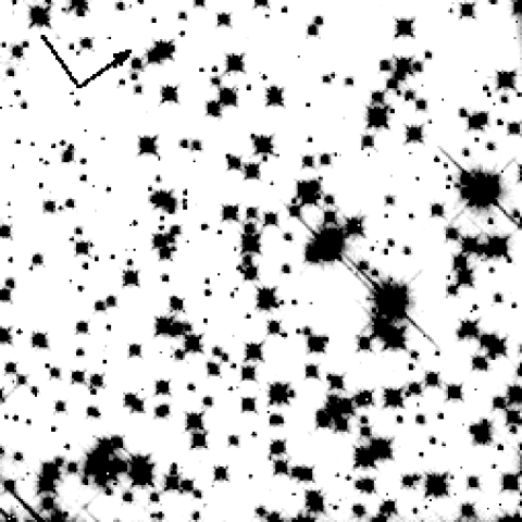
Figure 2: Negative image of the field FN 1 in the globular cluster M 4, located $\sim 1\mbox{${}^{\prime}\mskip-5.6mu.\,$}9$ away from the nominal cluster center, as observed with the F110W filter of the NIC 3 camera. The field covers $\sim 51$^′′ on a side. North is indicated by the arrow in the upper-left corner with East indicated to the left of North. The exposure time of the combined image is 3,840 s

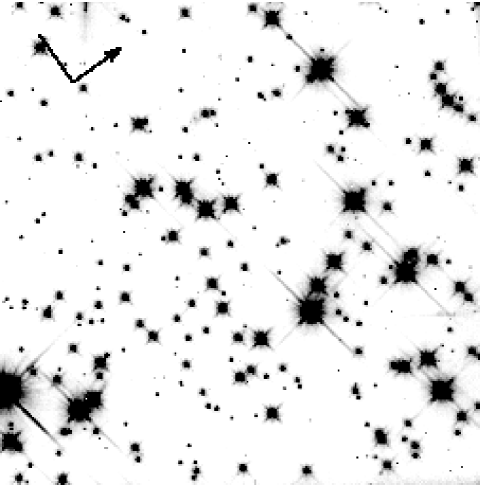
Figure 3: Same as Fig. 2 but for Field FN 2, located $2\mbox{${}^{\prime}\mskip-5.6mu.\,$}9$ away from the center of the cluster

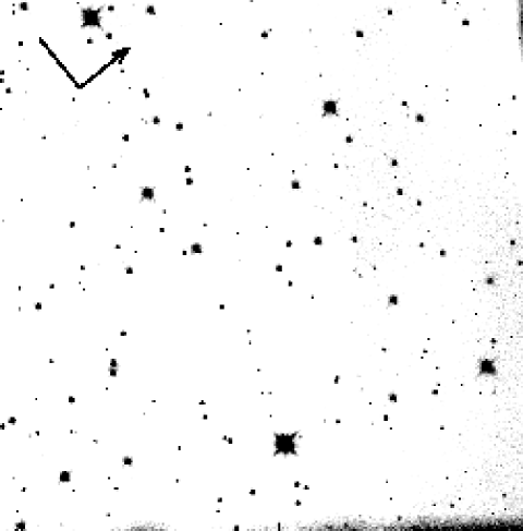
Figure 4: Same as Fig. 2 but for Field SKY

Photometry was carried out using the standard IRAF DAOPHOT package. The automated star detection routine daophot.daofind was applied to the frames, by setting the detection threshold at $5\,\sigma$ above the local background level. We have then examined by eye each individual object detected by daofind and discarded a number of features (PSF tendrils, noise spikes, etc.) that daofind had misinterpreted as stars, as well as a few extended objects whose full width at half maximum (FWHM) exceeded by a factor of two or more that typical of stellar objects in our frames (FWHM $\simeq 1.3$ pixel). As regards the saturation of bright objects, the CALNICA pipeline verifies whether and when the signal in each pixel, in the multiple readouts of each MULTIACCUM sequence, reaches the saturation or nonlinearity limit prior to the end of the exposure. All the samples which occur after the saturation limit are identified as bad and are not used in the final calculation of the mean count rate. This procedure should, in principle, allow one to measure fluxes in a wide dynamic range ($\sim\,10$ mag in our case).

A total of $466$, $332$ and $175$ objects respectively in the FN 1, FN 2 and SKY fields were identified and their fluxes measured with the PSF-fitting daophot.allstar photometry package, to derive the color–magnitude diagrams (CMD) for the three fields. The internal photometric accuracy has been estimated both with the IRAF phot task and through standard artificial–star experiments, giving similar results: better than $\pm 0.02$ mag for bright stars, degrading to about $\pm 0.3$ mag toward the detection limit at $m_{110}\sim 27$.

Instrumental magnitudes were calibrated and converted into the HST magnitude system (STMAG) using the relation:

$$m_{ST}=-2.5\log\left(\frac{c\,U}{\varepsilon}\right)-21.1$$ (1)

where $c$ is the count rate measured for each star, $U$ the inverse sensitivity of the instrumental setup (camera + filters), and $\varepsilon$ the encircled energy (i.e. the fraction of the total flux sampled by our photometry). In order to estimate the encircled energy $\varepsilon$, we have used five isolated, relatively bright stars, and have compared the flux measured by our photometry to their total flux, defined as that falling within a $2$^′′ radius. We have found in this way that, for our choice of aperture radius ($2.5$ pixel) and background annulus ($2.5\mbox{--}10$ pixel) the encircled energy amounts to $\simeq 90\,\%$ for both the F110W and F160W filters. Because the calibration of the NIC 3 camera is still preliminary, and the values of the inverse sensitivity $U$ are based on a limited set of spectrophotometric standards, we cannot convert very accurately our magnitudes from the STMAG system into any ground-based system. We, therefore, expect our absolute photometry to be accurate to within $10\mbox{--}15$ % (Colina & Rieke 1997). It is still possible, however, to translate our measurements into the VEGAMAG photometric system of the HST, defined as one in which the magnitude of Vega would be 0 in all bands and which is more similar to the classical Johnson–Cousin ground-based system. This can be done by simply subtracting the zero-point constants of $2.3$ mag and $3.7$ mag from the values of $m_{110}$ and $m_{160}$, respectively, thus obtaining the $J$ and $H$ magnitudes that we use hereafter.

The CMDs of all the objects identified in the three fields observed (FN 1, FN 2 and SKY) are shown in Figs. 5, 6, and 7. The MS is well defined in both cluster fields down to $J\simeq 20$, but below this level the stellar density decreases abruptly. In the SKY field, located $2^{o}$ away from the cluster center, the density of stars begins to increase for $J>20$, implying that the stellar population of the cluster becomes negligible at this point. Using the M–L relation of Baraffe et al. (1997), this point corresponds to $\sim 0.2$ M_⊙ for a distance modulus of $(m-M)_{\rm J}=11.86$. Another noticeable feature of the MS is the change of slope at $J\simeq 18$ corresponding to $M\simeq 0.5M_{\odot}$. This is because of the increasing infrared absorption of $H_{2}$ molecules in the stellar atmosphere which counteracts the reddening due to both the decreasing temperature and increasing metallic molecular absorption in the optical band (Baraffe et al. 1997). Below this limit, the MS becomes almost vertical.

The broadening of the MS for $J<16.5$ is greater than expected on the basis of the photometric errors alone. This broadening has been already noticed by Richer et al. (1995). Although it cannot be excluded that this feature is partly due to differential reddening (Alcaino et al. 1997) or to the presence of a binary sequence (Kroupa & Tout 1992; Ferraro et al. 1997), it seems more likely that this effect has to be ascribed to the non uniformity in the pixel response function of the camera (intra-pixel sensitivity) which has been shown to affect the photometry at the $10\%$ level in NIC 3 (Storrs 1998). On the other hand, the CMD of M 4 published by Kanatas et al. (1995) does not show this peculiar MS broadening. We have estimated that if the MS spread were to depend on the data processing alone, the actual error should be almost four times larger than the photometric uncertainty ($\sim 0.04$ mag) in the range $J<16.5$. As a consequence, it would be difficult to evaluate the age of the cluster from these data, but the LF of MS stars is little affected by this systematic effect.

We have superposed on the data shown in Figs. 5 and 6 the expected 10 Gyr, [M/H]$=-1.0$ theoretical isochrone (Chabrier & Baraffe 1997; Allard & Hauschildt 1997), as seen through the NICMOS filters F110W and F160W. For this comparison we have adopted for M 4 a color excess E(B–V)$=0.40$ and a distance modulus of $(m-M)_{\rm o}=11.51$ (Djorgovski & Meylan 1993). The ensuing values of the absorption in the F110W and F160W bands, estimated with the relation of Cardelli, Clayton, & Mathis (1989), are respectively $A_{110}=0.33$ and $A_{160}=0.18$. Although these values do not bring the theoretical models into perfect agreement with the observed CMD (an additional $\sim 0.1$ mag shift to the red seems to be required), we regard this mismatch as insignificant in light of the uncertainties on both the cluster’s parameters and theory. Moreover, there are indications of higher and variable values for $R_{V}$ (Vrba, Coyne, & Rapia 1993) towards the direction of M 4 which is behind the Sco–Oph dust complex. Thus, because the calibration of our filters is still preliminary, the match between observation and theory as shown in both the FN 1 and FN 2 fields (Figs. 5 and 6) is remarkable.

Figure 5: Color-magnitude diagram of the field FN 1 located $1\mbox{${}^{\prime}\mskip-5.6mu.\,$}9$ off the center of the globular cluster M 4 (NGC 6121). A total of 466 stars are detected and measured in two bandpasses (F110W and F160W) with the NIC 3 camera in this field. The solid line represents the expected theoretical MS from Baraffe et al. (1997). The magnitudes and colors in the HST-VEGAMAG system are shown respectively on the right and on the upper axis of the diagram. Photometric error bars are indicated on the left. The stellar masses determined by the M-L relationship of Baraffe et al. (1997) are indicated on the right side of the diagram

Figure 6: Same as Fig. 3 but for field FN 2, located $2\mbox{${}^{\prime}\mskip-5.6mu.\,$}9$ away from the center of the cluster. A total of 332 objects are measured in this field

Figure 7: CMD of the 175 objects in the field SKY at $\sim 2^{o}$ from the center of the cluster

The completeness of the sample has been evaluated by running artificial star tests in both bands. For each $0.5$ magnitude bin we have carried out 10 trials by adding a number of artificial stars not exceeding 10 % of the total number of objects in that bin and using a PSF derived directly from the co-added frames. These trials were followed recursively by daofind and allstar runs with the same parameters used in the reduction of the scientific images to assess the fraction of objects recovered by the procedure and the associated photometric error. Moreover, for each artificially added star, we compared the input magnitude with that at which the star was recovered, and found no systematic difference. In addition, the standard deviation of the magnitude values at which stars are recovered is in excellent agreement with the $1\,\sigma$ uncertainty of the photometric reduction, as estimated by the IRAF phot task, at all magnitude levels and is indicated on the left-hand side of the CMDs shown in Figs. 5, 6, 7.

The photometric completeness of the three observed fields is displayed in Fig. 8 as a function of the $m_{110}$ magnitude, whereas Table 2 lists, for each magnitude bin, the completeness fraction, the corrected LF, and the corresponding rms errors coming from the poissonian statistics of the counting process (all values of the LFs as well as their errors have been rounded off to the nearest integer).

Table 2: Luminosity function and completeness

	FN 1			FN 2			SKY
$m_{110}$	%	$N$	$\sigma_{N}$	%	$N$	$\sigma_{N}$	%	$N$	$\sigma_{N}$
17.25	100	14	4	100	6	2	100	0	0
17.75	99	26	4	99	9	3	100	0	0
18.25	98	30	6	99	11	3	100	1	1
18.75	97	54	8	98	28	5	100	1	1
19.25	95	40	7	98	26	5	99	0	0
19.75	94	41	7	96	19	4	99	2	1
20.25	92	35	6	96	18	4	98	2	1
20.75	89	36	7	95	20	5	98	1	1
21.25	87	26	6	94	23	5	98	7	3
21.75	83	55	9	91	24	5	98	11	3
22.25	82	29	6	90	16	4	97	8	3
22.75	78	27	6	88	16	4	97	13	4
23.25	74	22	6	85	15	4	96	17	4
23.75	70	17	5	81	21	5	94	13	4
24.25	66	26	7	75	23	6	93	12	4
24.75	58	13	5	66	23	6	88	25	6
25.25	51	18	7	66	33	8	84	19	5
25.75	41	20	7	55	32	9	78	19	5
26.25	32	9	6	37	22	9	66	30	8
26.75	20	15	11	26	11	9	51	33	10

Because we planned the NICMOS exposures in such a way that the F110W and F160W band images reach the same limiting magnitude with the same SNR, and because the colors of all the objects seen in the CMD (both cluster and field stars) span a very narrow range, all the objects identified in the F110W frames are also found in the F160W images and, therefore, the photometric completeness is similar in both bands.

Figure 8: Photometric completeness for the three observed fields. The completeness was calculated as the ratio of the numbers of the recovered stars $N_{r}$ and the added artificial stars $N_{a}$

To determine the stellar LF of M 4 at the locations corresponding to our fields FN 1 and FN 2 we have used the color and magnitude information derived from the CMDs in Figs. 5 and 6. Because M 4 is projected towards the Galactic bulge at a low Galactic latitude ($b\simeq 16$), the contamination due to field stars in FN 1 and FN 2 is expected to be significant. While at optical wavelengths it is often possible to disentangle the stars belonging to the cluster from those that do not simply on the basis of their color (see next section for a description of the “$2.5\,\sigma$ clipping” criterion), the colors of low-mass stars in the near-IR make this a very difficult undertaking. And indeed, both cluster and field stars share the same narrow color region in our F110W, F160W CMDs (see Figs. 5, and 6), with the latter scattered in luminosity because of their varying mass as well as distance. We had, however, expected this behavior (see Baraffe et al. 1997), and had therefore obtained a comparison field (SKY) at the same projected distance from the Galactic bulge as the FN 1 and FN 2 fields. Thus, the use of a control field is mandatory to reliably measure the stellar LF of this cluster, due to its unfavorable location.

Figure 9: The luminosity functions corrected for photometric incompleteness in the three observed fields, FN 1 (solid line), FN 2 (dashed line) and SKY (dash-dotted line)

We have measured the number of stars in each $0.5$ magnitude bin as a function of the $m_{110}$ magnitude along the MS in all three CMDs, discarding stars bluer than $J-H\simeq 0.4$ as they are clearly not MS objects. We have adopted exactly the same color selection also for the SKY field, so as to ensure the consistency of the comparison with the FN 1 and FN 2 fields data. Fig. 9 shows the LFs in the three observed fields FN 1 (continuous line), FN 2 (dashed line) and SKY field (dot-dashed line) after correction for photometric incompleteness as reported in Fig. 8 and Table 2. The artificial star tests indicate that at $J\sim 23$ on average more than 50 %, 60 %, and 80 % of the added stars are recovered respectively in the FN 1, FN 2, and SKY, thus implying statistically reliable LFs towards the H-burning limit at $\sim 0.1M_{\odot}$, corresponding to $J=22.5$ according to the M–L relations of Baraffe et al. (1997). In spite of the different crowding level and photometric completeness, the LFs measured in the adjacent fields FN 1 and FN 2 match each other very well, both showing peaks at $J\simeq 16.5$ and $J\simeq 19.5$. It is interesting to note that, after correction for incompleteness, all three LFs tend to a plateau for $J>21$, clearly marking in this way the bottom of the MS, from where field star contamination increases.

Figure 10: IR luminosity functions of M 4, obtained from our photometry and corrected for both incompleteness and contamination. The solid histogram represents the inner field (FN 1) LF whereas the dashed histogram reflects the outer field (FN 2).

Figure 11: The $m_{814},m_{555}-m_{814}$ CMD for the stars in the inner field FW 1 and in the external field FW 2

The final step in obtaining the LF of M 4 at these locations in the cluster is to subtract, after correction for photometric incompleteness, the SKY LF from the LFs measured in FN 1 and FN 2. The LF derived in this way is shown in Fig. 10 where the LFs in fields FN 1 (solid line) and FN 2 (dashed line) are corrected for incompleteness and contamination. The more external LF (FN 2) has been shifted vertically to reach the same maximum as the other. Within the observational errors, the two LFs are indistinguishable from one another.

2.2 The WFPC 2 data

HST–WFPC 2 observations of M 4 are available in the HST archive, from which we have retrieved two sets of F555W, F814W band images obtained in 1995 at $\sim 1\mbox{${}^{\prime}\mskip-5.6mu.\,$}3$ E (field FW 1) and $\sim 5^{\prime}$ SE (field FW 2) of the cluster center (see Fig. 1). Since field FW 1 contains our NICMOS FN 1 field, we are able to compare the LFs measured at the same location in different bands. In addition, field FW 2 provides information on the variation of the LF as a function of the radial distance.

The raw images were processed using the standard HST pipeline calibration. Images of the same field taken through the same filter were combined to remove cosmic ray hits and to improve the SNR of the data. The total exposure time of the combined images of field FW 1 corresponds to $15,000$ s in the F555W band and $5,500$ s in the F814W band. Exposure times for FW 2 are $31,500$  s and $7,200$ s respectively in F555W and F814W.

We have measured the fluxes of all the unresolved objects detected in these images by using almost the same photometric reduction technique employed for the NICMOS data (see Sect. 2.1), excluding the PC chips. In particular, we have run the automated star-detection routine daofind on the combined frames to detect objects rising at least $5\,\sigma$ above the local average background. Each of the detected objects has been visually examined and the spurious identifications, due essentially to the diffraction spikes of a number of saturated stars, were removed from the output list. In this way a total of $1439$ and $1078$ unsaturated objects were detected, respectively in fields FW 1 and FW 2.

The photometric routines phot and allstar were used to measure the fluxes of the objects detected in such a way on the single frames. The PSF was modeled by averaging moderately bright stars for each frame. The instrumental magnitudes from the different frames were weighted by the inverse square of their uncertainties, averaged for each filter and converted to the instrumental magnitudes of the combined images.

We calculated the aperture correction for each WF chip in the two fields, using a diameter size of 1^′′ and transformed the final instrumental magnitudes into the VEGAMAG photometric system adopting the updated zero points listed in the November 1997 edition of the HST Data Handbook.

Fig. 11 displays the $m_{814},m_{555}-m_{814}$ CMDs for all objects of the inner field FW 1 and of the external field FW 2. The completeness corrections have been estimated by running artificial star tests in both bands and in the combined images for each WF chip. The procedure is essentially the same as described in Sect. 2.1. Our simulations indicate that in the inner field at $m_{814}\simeq 21$ on average about $90\%$ of the artificial stars are recovered. In the outer field, the same completeness level is reached at $m_{814}\simeq 22$ due to the lower crowding.

Figure 12: a WFPC2 CMD of the 193 objects in common with the NICMOS FN 1 field. b NIC3 CMD of the same objects. Crosses represent white dwarfs, asterisks field stars, and circle cluster members

Fig. 12 shows the NICMOS and the WFPC 2 CMDs of the 193 stars common to both inner fields. The center of the overlapping region is located $\sim 1\mbox{${}^{\prime}\mskip-5.6mu.\,$}9$ NE of the cluster center. The crosses represent objects already identified as white dwarfs (WD) by Richer et al. (1997) on the basis of the agreement between observational and theoretical loci of a $0.5$M_⊙ Hydrogen-rich WD cooling sequence, the asterisks indicate objects which, lying outside the narrow cluster MS, probably belong to the foreground whereas the circles mark the cluster members.

As a first result we have the observational confirmation of the contamination of the cluster MS in the infrared due to field stars: it is impossible to follow the MS in the IR bands all the way to its very bottom without a statistical decontamination through the use of an external field or excluding the foreground stars using proper motion data.

Secondly, the cross–identification of the stars in both the WFPC 2 and NICMOS photometry tables enables us to identify in a globular cluster for the first time an infrared WD sequence. In the F110W band the WDs are distributed in a color sequence instead of a luminosity sequence as in the optical CMD. This is an important observational constraint for the modeling of the atmosphere of cool WDs. Bergeron, Saumon, & Wesemael (1995) have shown that the cool WDs with mixed $H/He$ chemical composition can be easily recognized from their predicted strong infrared flux deficiency.

Adopting the $2.5\,\sigma$ clipping criterion (De Marchi & Paresce 1995), from the CMDs of Fig. 11 we have measured the LF of MS stars by counting the objects in each $0.5$ mag bin and within $\pm 2.5$ times the $m_{555}-m_{814}$ color standard deviation around the MS ridge line. The WFPC 2 LFs of both observed fields, corrected for incompleteness and field star contamination, are shown in Fig. 13. The exposure times of the WFPC2 frames were calculate to reach the very end of the MS and, as a consequence, the saturation effect does not allow us to evaluate reliable LFs at $m_{814}<19$ while the foreground contamination cuts them at $m_{814}>22.5$.

3 The luminosity and mass functions

Fig. 14 shows the F814W LFs of the two WFPC 2 fields located at $\sim 2\arcmin$ (triangles) and at $\sim 6\arcmin$ (boxes) from the cluster center, together with the NICMOS LF (diamonds) converted into the F814W band using the Baraffe et al. (1997) M-L relationships appropriate for the metallicity of M 4 ($[M/H]=-1$, i.e. $[Fe/H]\simeq-1.3$; Harris 1996) as a function of the absolute $M_{814}$ magnitude. Through the theoretical M-L relations, we can associate a mass to each of the magnitude bins that appear in the NICMOS LF. Then, by also knowing the M-L relation for the F814W band, we can easily translate the center of the magnitude bins from the F110W magnitude scale to the F814W band and adjust the width of the bins themselves to reflect the different slope of the M-L relations in the magnitude range covered by each bin.

Within the error bars, in the overlapping range, the inner NICMOS and inner WFPC 2 LFs show the same trend: the overall LF is relatively flat or slightly decreasing in the range $4<M_{814}<8$ and decreases steeply beyond that point. The agreement between the two LFs measured in the visible (F814W) and in the near IR (F110W), in spite of the small size of the observed sample, confirms the robustness of our photometric reduction and the reliability of the M–L relations used to translate the IR data to the visible (see also De Marchi 1999 on this issue).

Figure 13: Luminosity functions of the fields FW 1 (triangles) and FW 2 (squares) after correction for incompleteness and field star contamination

Figure 14: Logarithm of the WFPC2 $2\arcmin$ (triangles) and $6\arcmin$ (boxes) LFs in the F814W band together with the NICMOS LF (diamonds) translated to F814W adopting M-L relations of Baraffe et al. (1997). Solid lines represent the fit obtained using a power-law with exponent $x=-0.8$ in the inner field. As regards the outer field, the LF is reproduced using a two-segment power-law, with exponents $x=1$ down to $M_{814}\simeq 8.5$ and $x=-0.3$ down to the detection limit

On the other hand, the WFPC 2 LF measured $6\arcmin$ away from the center ($\simeq 1.6r_{\rm hm}$; Harris 1996) shows a different shape, in that it increases with decreasing luminosity up to a peak at $M_{814}\simeq 9$ and from there it drops all the way to the MS detection limit at $M_{814}\simeq 10.5$. This behavior is typical of all the GCs observed so far with the HST at or near the half-mass radius (Paresce, De Marchi & Romaniello 1995; De Marchi & Paresce 1995a, 1995b, 1996, 1997; Cool, Piotto, & King 1996; King et al. 1997; Pulone, et al. 1998, De Marchi 1999) and is related to an extremum in the derivative of the mass-absolute magnitude relation of the low mass stars as discussed in Kroupa & Tout (1997).

Thus, the obvious difference between the inner and outer LFs should be compatible with the dynamical modifications of a GC as a result of mass segregation due to energy equipartition through two-body relaxation (Spitzer 1987). Indeed, it is expected that more massive stars give up part of their kinetic energy to lighter stars during close encounters and sink towards the cluster center. This effect would explain qualitatively why massive stars are relatively more numerous at $2\arcmin$ from the center than they are near the half-mass radius. We address this issue in more detail in Sect. 4.

Under the assumption that the MF of the stellar population at $2\arcmin$ from the cluster center is represented by an exponential distribution of the form:

$$dN\propto m^{-x}d\log m$$ (2)

and using the M-L relation of Baraffe et al., we can reproduce rather accurately the inner LF in Fig. 14 with an exponent $x=-0.8\pm 0.4$ (solid line). The outer LF, however, cannot be fit by any single exponent power-law distribution, regardless of the adopted slope, as no such function can reproduce the peak observed at $M_{814}\simeq 9$. A reasonable fit can be obtained using a mass function which rises as a power-law with $x=1$ down to $\sim 0.25M_{\odot}$ ($M_{814}=8.5$) and then drops all the way to the MS detection limit with an exponent $x=-0.3$. Unfortunately the lack of data at the bright end of the WFPC2 LF, due to saturation, does not allow us to constrain the MF slope in the mass interval which is most sensitive to dynamical effects, although the comparison between the inner and outer mass functions at lower masses already suggests strong mass segregation.

4 The dynamical state of M 4

Addressing the question as to whether the difference between the inner and outer MFs described above can be quantitatively accounted for by the two-body relaxation mechanism requires a simulation of the dynamical structure of the cluster. We have used multi-mass King-Michie models, constructed with an approach nearly identical to that of Gunn & Griffin (1979), as described in Meylan (1987, 1988). Each model is characterized by an IMF in the form of an exponential as in Eq. (3), with an exponent $x$ which is not necessarily constant (i.e. $x$ is allowed to vary with mass; see details below), and by three structural parameters describing respectively the scale radius ($r_{\rm c}$), the scale velocity ($v_{\rm s}$) and the central value of the dimensionless gravitational potential $W_{\rm o}$. We have assumed complete isotropy in the velocity distribution.

Because King-Michie modeling provides a “snapshot” of the current dynamical status of the cluster rather than its evolution, it is useful to define the mass distribution of cluster stars at present (global MF; GMF) as the MF that the cluster would have simply as a result of stellar evolution (i.e. ignoring any local modifications induced by internal dynamics and/or the interaction with the Galactic tidal field). Clearly, the IMF and GMF of MS (unevolved) stars is the same. For practical purposes, the GMF has been divided into sixteen different mass classes, covering MS stars, white dwarfs, and heavy remnants. All stars lighter than $0.8M_{\odot}$ have been considered still on their MS, while heavier stars with initial masses in the range $[8\mbox{--}100]$ M_⊙ have been assigned a final (i.e. post-evolution) mass of $1.4$ M_⊙. White dwarfs have been divided into three classes, according to their initial masses, following the prescriptions of Weidemann (1987) and Bragaglia, Renzini, & Bergeron (1995). Although the analytical form we adopted for the IMF would allow the exponent $x$ of the GMF to vary, we have initially restricted our investigation to the single exponent case.

From the parameter space defined in this way, we have extracted only those models that simultaneously fit both the observed surface brightness (SBP) and velocity dispersion (VDP) profiles of the cluster. The fit to the SBP and VDP, however, can only constrain $r_{\rm c}$, $v_{\rm s}$, and $W_{\rm o}$, while still allowing the IMF to take on a variety of shapes. It is precisely to attempt to break this degeneracy that we impose the condition that the model GMF agree with the observed LFs. We note here that the local MF at any given place inside the cluster originates from the GMF and stems directly from imposing the condition that stars of different masses be in thermal equilibrium with each other.

In our simulations, we have used the VDP determined by Peterson, Rees, & Cudworth (1995). Concerning the SBP, we have compared the profile measured by Kron, Hewitt, & Wasserman (1984) with that of Trager, King, & Djorgorvski (1995) and found some discrepancies. We have, therefore, adopted an average SBP, defined as the parameterized King-type profile (King 1962) that corresponds to the canonical values of core radius $r_{\rm c}=50$^′′ and concentration $c=1.6$ (Harris 1996; note, however, that values as large as $r_{\rm c}\simeq 90$^′′ and $c\simeq 2$ are found in the literature, as discussed below). The canonical SBP defined in this way gives a reasonable fit to both measurements, and we have used the least squares between the canonical profile and the observations of Kron et al. (1984) and Trager, King, & Djorgorvski (1995) as an estimate of the errors.

Although several models are able to reproduce the observed radial profiles (SBP and VDP) reasonably well, no choice of the exponent $x$ gives local MFs that, converted into LFs using the M-L relation described above, agree with the data shown in Fig. 14. In fact, our simulations show that an IMF like the one given in Eq. (3) cannot simultaneously fit the LFs at $2\arcmin$ and $6\arcmin$ radial distance, regardless of the value of the exponent $x$, although each LF can individually be approximated with a power-law IMF with index $x\simeq-0.8$ for the LFs at $2\arcmin$ radius and $x\simeq 0.4$ at $6\arcmin$. (In the latter case, however, the fit is not good at magnitudes fainter than $M_{814}\simeq 9$). As an example, in Fig. 15 we show the theoretical LFs (solid lines) corresponding to the model that best fits the observations at $6\arcmin$: at bright magnitudes (i.e. for masses $>0.3$ M_⊙ ) the model LF systematically deviates from the observational data at $2\arcmin$ by far more than the experimental errors.

Figure 15: The WFPC2 $2$′(triangles) and $6$′(squares) LFs, the NICMOS LF (diamonds) in the F814W band, compared with the theoretical LFs at the same distances, obtained by the mass stratification of the dynamical model described in the text. The slope of the main sequence mass segment of the GMF is $x=0.4$. The core radius and the concentration of the parameterized SBP are $r_{rmc}=50$^′′ and $c=1.6$

A single-exponent power-law distribution, however, is only a rough approximation to the IMF, particularly at the low-mass end (see Scalo 1998). And indeed, the deepest LFs today available for NGC 6397 (Paresce, De Marchi, & Romaniello 1995; King et al. 1998) and NGC 6656 (De Marchi & Paresce 1997) suggest that the MF could flatten out below $\sim 0.25$ M_⊙ and possibly drop (in the logarithmic plane). We have, therefore, run some simulations with an IMF that follows an exponential law with two values of the exponent: $x$ is positive for masses $m>0.25$ M_⊙ and zero below that mass. Not even in this case, however, does the predicted shape of the MF at $\sim 2\arcmin$ and $\sim 6\arcmin$ from the center match the observations simultaneously, regardless of the value of $x$ for masses $m<0.25$ M_⊙ .

Although we could explore other possible shapes of the IMF, it is unlikely that its form can largely deviate from some sort of a slowly varying exponential. Thus, if we judge that King-Michie modeling is a viable way to describe the dynamical state of M 4, we have to conclude that some of the constraints that we are forcing into the models are not correct, i.e. that the SBP or the VDP (or both) are not compatible with the LFs that we measured and which seem rather robust (see Sect. 3).

We have, therefore, investigated the origin of the discrepancy between the observed LFs and the local MFs produced by the models starting from plots similar to that shown in Fig. 15. We have noticed that, if we begin by fixing the exponent (exponents) of the IMF in such a way that the local MF agrees with our measurements at $6\arcmin$ from the center, we are tempted to conclude that the scale radius of our models is too small. Fixing the exponent in that way is a reasonable assumption, since both theoretical and semiempirical arguments suggest that near the cluster half-mass radius ($\sim$ half-light $\sim 3.7$′; Harris 1996), the local MF should only marginally differ from the IMF (Richer et al. 1991; Vesperini & Heggie 1997).

In fact, in order for the model LF to reproduce the LFs measured at $2\arcmin$, the former has to decrease monotonically with luminosity, and this is precisely what has been shown to take place in the innermost cluster regions (see Paresce, De Marchi, & Jedrzejewski 1995; King, Sosin, & Cool 1995; De Marchi & Paresce 1996). In other words, we would need a scale radius ($r_{\rm c}$) sufficiently large so as to place the region at $r\simeq 2$′ still close enough to the center that the LF of its stellar population is compatible with an inverted function. The canonical value of $r_{c}=50$^′′ is not large enough for this to happen.

Figure 16: The same as Fig. 15 when adopting as GMF a power-law with exponents $x=0.2$, in the range $0.8\mbox{--}0.25$ M_⊙ , and $x=-0.4$ for masses $<0.25$ M_⊙ 

Figure 17: The same as Fig. 15 when the radial LFs are fitting a SBP with $r_{\rm c}=92$^′′ and $c=1.9$. The adopted GMF has main sequence slopes $x=1$, in the range $0.8\mbox{--}0.25$ M_⊙ , and $x=-0.4$ for masses $<0.25$ M_⊙ 

Through repeated trials, we have found that by forcing the core radius $r_{\rm c}$ to take on the value of $\sim 90$^′′ (a figure still compatible with the measurements of Peterson & King (1975) suggesting $r_{\rm c}\simeq 93$^′′ from the fit to their SBP) both sets of LFs can be simultaneously fit by an exponential IMF with index $x\simeq 0.2$ in the range $0.8\mbox{--}0.25$ M_⊙ and which drops with $x\simeq-0.4$ at lower masses (Fig. 16). The values of the concentration ratio ($c\simeq 1.5$), the total cluster mass($\simeq 8.8\times 10^{4}$ M_⊙ ), and the index of the IMF above $0.8$ M_⊙ ($x\simeq 1.4$) are also reasonable. In the mass range $0.2-0.6$ M_⊙ , the slope of the IMF suggested by this model is shallower than the $x\simeq 1$, value proposed by De Marchi & Paresce (1997) for NGC 6397 and NGC 6656. Nevertheless, it would still be possible to find a model (Fig. 17) that uses the IMF of De Marchi & Paresce (1997) and simultaneously fits the LFs observed at $\sim 2\arcmin$ and $\sim 6\arcmin$, and this would require the core radius to grow to $\sim 90$^′′ and the concentration parameter to take on the value of $c\simeq 1.9$ (both values still compatible with the data of Peterson & King (1975) and Kron et al. (1984), respectively). The difference between the IMFs used in Figs. 16 and 17 and between the set of parameters defining our models can be taken as an indication of the uncertainties affecting our approach, and can be traced back to the indetermination accompanying the SBP and the ensuing value of $r_{\rm c}$. It also shows how difficult it is to infer the shape of the GMF starting from the observations when the knowledge of the structural parameters of the cluster is so uncertain.

We would also like to point out that the results given above and shown in Figs. 16 and 17 should anyhow be taken with care: they stem from the assumption that King-Michie modeling with the limitations that we applied to it is adequate to describe the dynamical state of M 4, and therefore the good fits that we obtain do not necessarily guarantee that these models reflect the physical state of the cluster. And indeed, from the kinematics of its orbit (Dauphole et al. 1996) one would argue that M 4 should have undergone extensive tidal stripping and shocks since it penetrates very deeply into the Galactic bulge and its orbital plane is one of the closest to the Galactic disk. These effects might have strongly modified the local mass distribution (particularly in the outer regions) and the two-body relaxation mechanism that we adopted could no longer apply. We are grateful to Pavel Kroupa, the referee, for having pointed out that, among the possible problems with the assumptions underlying our modeling, there is the assumed complete isotropy in the velocity distribution of the cluster members. Stellar-dynamical modeling of isolated globular clusters shows that the velocity dispersion becomes anisotropic as a function of time (see Fig. 4e in Spurzem & Aarseth 1996). Models that include a tidal field, however, suggest that the anisotropy is reduced because of rapid loss of stars having radial orbits (Takahashi, Lee, & Inagaki 1997). Nevertheless, it is not clear if the tidal field is realistically taken account of in the Takahashi et al. (1997) Fokker-Planck models, since in the above mentioned Fig. 4e of Spurzem & Aarseth (1996) it can be seen that the anisotropy would also be pronounced well inside the tidal radius. Moreover, GCs may be born with a significant anisotropic velocity dispersion (Aarseth, Lin, & Papaloizu 1988).

With this caveat in mind, we can quantitatively conclude that the LFs observed at $\sim 2\arcmin$ and $\sim 6\arcmin$ away from the center of M 4 can be traced back to the same GMF, which appears to have been locally modified as a result of mass segregation due to two body relaxation. The underlying IMF is most likely represented by a slowly rising exponential ($x\simeq 0.2\mbox{--}1$) that flattens out and possibly drops below $\sim 0.25$ M_⊙ . Any attempt to better define the shape of the IMF and to characterize more thoroughly the relaxation mechanism would require a more precise measurement of the surface brightness (or, better, radial density) profile and the observation of the LF of MS stars at four or five locations inside the cluster, so as to simultaneously constrain both the core radius (for a given mass class) and the mass spectrum of all luminous objects as a function of the distance from the center. This project can be efficiently and effectively carried out with a wide field imager at a 10-m class telescope like the VLT.

5 Summary

Our main conclusions can be summarized as follows:

1. We have measured the visible and infrared LFs of M 4 at $2$′and $6$′ from the cluster center down to $I\simeq 10$ with photometric completeness always better than 50%.

2. The LFs measured at $2\arcmin$ with the two instruments agree very well with each other and show a slow decrease with luminosity.

3. The LF measured with the WFPC2 at $6$′ radial distance shows an increase with decreasing luminosity up to a peak at $I\simeq 9$ followed by a drop all the way to the detection limit.

4. The difference between the two sets of LFs is qualitatively compatible with the effects of mass segregation. It can, however, be quantitatively reproduced using a King-Michie model only when adopting cluster structural parameters which, although compatible with those available in the literature, deviate from their canonical value. The IMF required for the model to fit has an exponential slope of $\sim 0.2\mbox{--}1.0$ in logarithmic mass units between $0.2$ and $0.8$ M_⊙ .

5. Our observations require that the IMF determined in this way flatten out and possibly drop below $0.2$ M_⊙ .

6. For the first time an infrared WD sequence has been unambiguously identified in a globular cluster. The WD locus appears to be a color sequence instead of a luminosity sequence as in the optical.

- (1) Aarseth S.J., Lin D.N.C., Papaloizou J.C.B., 1988, ApJ 324, 288
- (2) Adams F.C., Fatuzzo M., 1996, ApJ 464, 256
- (3) Alcaino G., Liller W., Alvarado F., et al., 1995, AJ 114, 189
- (4) Allard F., Hauschildt P., 1997, in preparation
- (5) Baraffe I., Chabrier G., Allard F., Hauschildt P., 1997, A&A 327, 1054
- (6) Bergeron P., Saumon D., Wesemael F., 1995, ApJ 443, 764
- (7) Bragaglia A., Renzini A., Bergeron P., ApJ 443, 735
- (8) Cardelli J.A., Clayton G.C., Mathis J.S., 1989, ApJ 345, 245
- (9) Chabrier G., Baraffe I., 1997, A&A 327, 1039
- (10) Chabrier G., Méra D., 1997, A&A 328, 83
- (11) Colina L., Rieke M.J., 1997, In: Casertano S., et al. (eds.) HST Calibration Workshop. Space Telescope Science Institute
- (12) Cool A.M., Piotto G., King I.R., 1996, ApJ 468, 655
- (13) Dauphole B., Geffert M., Colin J., et al., 1996, A&A 313, 119
- (14) Davidge T., Simons D., 1994, ApJ 423, 640 DS
- (15) De Marchi G., Paresce F., 1995a, A&A 304, 202
- (16) De Marchi G., Paresce F., 1995b, A&A 304, 211
- (17) De Marchi G., Paresce F., 1996, ApJ 467, 658
- (18) De Marchi G., Paresce F., 1997, ApJ 476, 19
- (19) De Marchi G., 1999, AJ, in press
- (20) De Marchi G., Paresce F., 1997, ApJ 476, L19
- (21) Djorgovski S.G., 1993, In: Djorgovski S.G., Meylan G. (eds.) Structure and Dynamics of Globular Clusters. ASP Conf. Ser. 50, ASP, San Francisco, 273
- (22) Ferraro F.R., Caretta E., Fusi Pecci F., Zamboni A., 1997, A&A 327, 598
- (23) Gnedin O.Y., Ostriker J.P., 1997, ApJ 474, 223
- (24) Gunn J.E., Griffin R.F., 1979, AJ 84, 752
- (25) Harris W.E., 1996, AJ 112, 1487
- (26) Kanatas I.N., Griffiths W.K., Dickens R.J., Penny A.J., 1995, MNRAS 272, 265
- (27) King I.R., 1962, AJ 67, 471
- (28) King I.R., Sosin C., Cool A.M., 1995, ApJ 452, L33
- (29) King I.R., Anderson J., Cool A.M., Piotto G., 1998, ApJ 492, L37
- (30) Kron G.E., Hewitt A.V., Wasserman L.H., 1984, PASP 96, 198
- (31) Kroupa P., Tout C.A., 1992, MNRAS 259, 223
- (32) Kroupa P., Tout C.A., 1997, MNRAS 287, 402
- (33) MacKenty J., et al., 1997, In: MacKenty J., et al. (eds.) NICMOS Instrument Handbook. STScI, Baltimore
- (34) Meylan G., 1987, A&A 184, 144
- (35) Meylan G., 1988, A&A 191, 215
- (36) Paresce F., De Marchi G., Jedrzejewski R., 1995, 442, 57L
- (37) Paresce F., De Marchi G., Romaniello M., 1995, ApJ 440, 216
- (38) Peterson R.C., Rees R.F., Cudworth K.M., 1995, AJ 443, 124
- (39) Peterson C.J., King I.R., 1975, AJ 80, 427
- (40) Pulone L., De Marchi G., Paresce F., Allard F., 1998, ApJ 492, L41
- (41) Richer H.B., Fahlman G.G., Buonanno R., et al.,1991, 381, 147
- (42) Richer H.B., Fahlman G.G., Ibata R.A., et al., 1995, ApJ 451, L17
- (43) Richer H.B., Fahlman G.G., Ibata R.A., et al., 1997, ApJ 484, 741
- (44) Scalo J., 1998, astro–ph/9712317
- (45) Spitzer L. Jr., 1987, Dynamical Evolution of Globular Clusters. Princeton University Press, Princeton, New Jersey
- (46) Stetson P.B., 1987, PASP 99, 191
- (47) Storrs A.D., 1998, Instrument Science Report. NICMOS-98-006, STScI, Baltimore
- (48) Spurzem R., Aarseth S.J., 1996, MNRAS 282, 19
- (49) Takahashi K., Lee H.M., Inagaki S., 1997, MNRAS 292, 331
- (50) Trager S.C., King I.R., Djorgovski S., 1995, AJ 109,218
- (51) Vesperini E., Heggie D.C., 1997, MNRAS 289, 898
- (52) Vrba F.J., Coyne G.V., Rapia S., 1993, AJ 105, 1010
- (53) Weidemann V., 1987, A&A 188, 74