The origin of carbon, investigated by spectral analysis of solar-type stars in the Galactic Disk^⋆

Abstract

Abundance analysis of carbon has been performed in a sample of 80 late F and early G type dwarf stars in the metallicity range $\mathrm{-1.06\leq[Fe/H]\leq 0.26}$ using the forbidden [C i] line at $8727\mbox{{\AA}}$. This line is presumably less sensitive to temperature, atmospheric structure and departures from LTE than alternative carbon criteria. We find that $\mathrm{[C/Fe]}$ decreases slowly with increasing $\mathrm{[Fe/H]}$ with an overall slope of $-0.17\pm 0.03$. Our results are consistent with carbon enrichment by superwinds of metal-rich massive stars but inconsistent with a main origin of carbon in low-mass stars. This follows in particular from a comparison between the relation of $\mathrm{[C/O]}$ with metallicity for the Galactic stars and the corresponding relation observed for dwarf irregular galaxies. The significance of intermediate-mass stars for the production of carbon in the Galaxy is still somewhat unclear.

1 Introduction

The stellar origin of carbon became clear with the discovery of the Triple Alpha reaction (Öpik 1951; Salpeter 1952) and the beautiful demonstration by Hoyle Hoyle (1954) that the high carbon abundance would require a resonance state at $7.65\mbox{MeV}$ of carbon, a prediction that was soon verified experimentally. But in which type of stars was carbon formed?

In their classical paper Burbidge et al. Burbidge et al. (1957) suggested carbon to be provided by mass loss from red giants and supergiants. Arnett & Schramm Arnett and Schramm (1973) argued that massive stars might be most effective. They discussed the composition of matter estimated to be ejected from stars (with helium core masses above $4\mathcal{M}_{\odot}$, i.e. $\mathrm{\mathcal{M}_{tot}\geq 10\mathcal{M}_{\odot}}$) and found $\mathrm{C/O}$ ratios consistent with the solar system values. The yield prescriptions developed by Talbot & Arnett (1973, 1974) consequently ascribed carbon production to the massive stars. However, Truran Truran (1977) and Tinsley Tinsley (1977) argued that carbon stars of lower mass could also be significant sites for carbon. Dearborn et al. Dearborn et al. (1978) also suggested that low mass stars (as evidenced by carbon stars and carbon-rich planetary nebulae) may be a significant source of ${\rm\,{}^{12}C}$, while Iben & Truran Iben and Truran (1978) concluded from thermally pulsing models that intermediate mass stars and high mass stars contributed carbon in roughly equal amounts. The arguments for significant contributions of carbon by low-mass and intermediate-mass stars were further elaborated by Tinsley Tinsley (1978) and Sarmiento & Peimbert Sarmiento and Peimbert (1985). Timmes et al. Timmes et al. (1995) in their models of Galactic chemical evolution with then available yields for supernovae as well as for low- and intermediate mass stars, found very significant contributions of carbon from the latter to the Galactic Disk. (For a general review on the significance of low- and intermediate-mass carbon stars for Galactic nucleosynthesis, see Gustafsson & Ryde (1998).) Recently, Kobulnicky & Skillman Kobulnicky and Skillman (1998) concluded from the correlation between $\mathrm{C/O}$ and $\mathrm{N/O}$ ratios found in H ii regions in three starforming galaxies, that the formation of N and C is coupled and presumably occurs in intermediate or low mass stars. Prantzos et al. Prantzos et al. (1994), however, adopting the idea of Maeder Maeder (1992) that radiatively driven massive winds from high-mass stars should provide huge amounts of helium and carbon, found these stars to be the main contributors while the role of intermediate-mass stars seemed much less significant. Similarly, Garnett et al. Garnett et al. (1995) observed that the C/O ratio increased with increasing O/H for dwarf irregular galaxies, a trend which they found to be consistent with the suggestion that carbon is produced in massive stars with yields dependent on metallicity, as is expected for stars with radiatively driven winds.

The shifting views as regards the relative role of high-mass, intermediate-mass and low-mass stars have reflected the different uncertainties and conjectures concerning the carbon production, dredge-up and mass loss from stars of different mass and metallicity. Although considerable progress has been made in these respects, there are still very severe remaining uncertainties. Also as regards observed carbon abundances for stars and planetary nebulae the uncertainties have been, and are still, considerable which makes checks of the theoretical results, as well as more direct empirical approaches, difficult. We shall here present an attempt to improve in this latter respect, as regards carbon abundances for solar-type stars in the Galactic Disk. The idea is to use high S/N observations of a hitherto little used forbidden carbon line in the infrared as the single criterion. The strength of this line, in comparison with other carbon abundance criteria, is not at all as sensitive to other parameters as to the carbon abundance. We shall also see that with high quality data it is possible to carry out more direct tests concerning the role of stars of different masses; tests that are independent on the results of the calculations of yields.

2 Observations and data reductions

The observations were made at European Southern Observatory (ESO) with the $1.4\mbox{m}$ Coudé Auxillary Telescope (CAT) coupled to the Coudé Echelle Spectrometer (CES) and the Long Camera during 3 observing runs with the following CCD detectors: July 2-15 1994 CCD#30, Dec 29 1994-January 4 1995 CCD#34 and Sept 14-26 1995 CCD#34. The slit-viewing auto-guiding system ensured efficient light collection. The focusing and alignment of the CCD cameras were checked before each observing night.

Spectra centered near the $8727\mbox{{\AA}}$ [C i] line and with a wavelength range of about $70\mbox{{\AA}}$ and a resolution of 65,000 were obtained for 87 southern stars of the Edvardsson et al. Edvardsson et al. (1993) (cited as EAGLNT in the following) survey with different metallicities. Depending on the stellar magnitudes and weather conditions integrations of between 20 seconds (Procyon, $V=0.37$) and 8 times 60 minutes (HD 199289, $V=8.29$) were obtained for the stars. The long integration times were motivated by the need to obtain high S/N ratios (preferably above 200) for the generally very weak [C i] line. In order to increase the S/N ratio, slightly different central wavelengths were chosen for separate observations of the same star. A typical S/N ratio for the final, summed up spectra was generally between 200 and 300. No spectrum had a S/N ratio below 150.

The data reductions were performed either on line with the ESO IHAP software or later with the ESO MIDAS package, and contained the following steps:

• Subtraction of bias and dark signal from the stellar frames and of bias from the flat-field frames.

• Division of the stellar frame by a flat-field frame obtained with unaltered set-up, and within hours of the stellar frame.

• Summation of the relevant CCD rows to produce a one-dimensional spectrum.

• Wavelength calibration by means of a Th/Ar lamp spectrum obtained in connection with the stellar frame.

• A 3rd order spline function was fitted to the pre-defined continuum points in the spectrum, and finally the spectrum was divided by this function to yield a relative flux scale with continuum level of $1.00$.

For stars where more than one spectrum of the region was obtained, both the individual spectra and also the rebinned and summed total spectrum were alternatively used in the data analysis.

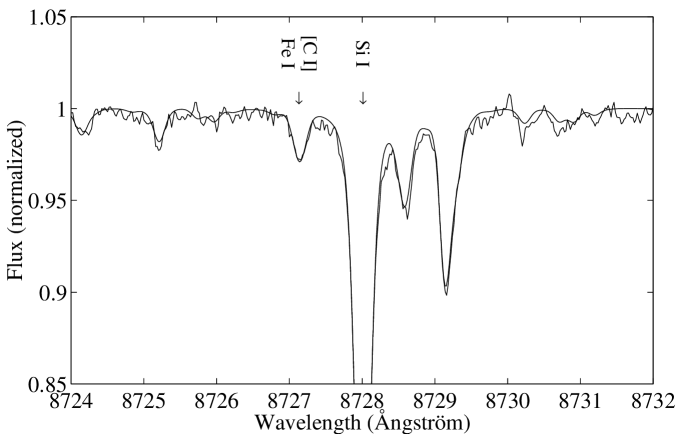
Figure 1: The observed and synthetic spectra of HR 1294 (HD 26491) with the carbon, iron and silicon lines indicated

3 Analysis

3.1 Model atmospheres

The stellar spectra were synthesised with the Uppsala spectrum synthesis program, using the opacity-sampling MARCS model atmospheres described in EAGLNT. These are line-blanketed, one-dimensional atmospheres with mixing-length convection, produced under the assumption of LTE. An example of a comparison between observed and synthetic spectra is shown in Fig. 1.

3.2 Atmospheric parameters

Originally, the atmospheric parameters $T_{\mathrm{eff}}$, $\log g$ and $\mathrm{[Fe/H]}$ of EAGLNT were adopted, and $\xi_{\mathrm{t}}$ was calculated with the formula given in EAGLNT

$$\xi_{\mathrm{t}}=1.25+8\cdot 10^{-4}(T_{\mathrm{eff}}-6000)-1.3(\log g-4.5)\mbox{km\,s${}^{-1}$}.$$ (1)

In EAGLNT, the surface gravities ($g_{\mathrm{phot}}$) were based on the $c_{\mathrm{1}}$ index of the Strömgren photometry. However, surface gravities were alternatively estimated for the stars from the parallaxes given in the HIPPARCOS catalogue ESA (1997) using the equation

$$\log g_{\pi}=4\log\frac{T_{\mathrm{eff}}}{T_{\mathrm{eff}}^{\odot}}+\log\frac{\mathcal{M}}{\mathcal{M}_{\odot}}+2\log\pi+$$

$$0.4(V+BC-0.26)+4.44.$$ (2)

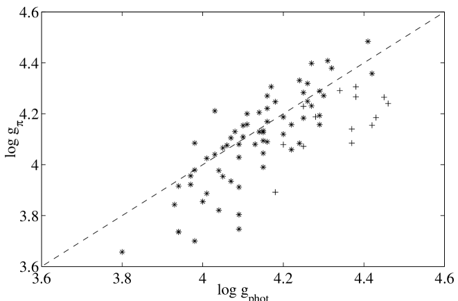
Figure 2: Comparison between $\log g_{\mathrm{phot}}$ given in Edvardsson et al. (1993) (EAGLNT) and $\log g_{\mathrm{\pi}}$ estimated from Hipparcos parallaxes. The plusses represent stars with $\mathrm{[Fe/H]}\leq-0.6$. The dashed line indicates a one-to-one relation to guide the eye

The masses for the stars were estimated from evolutionary tracks by Schaller et al. Schaller et al. (1992) and Claret & Gimenez Claret and Gimenez (1992). Due to the uncertainty in the models and the few tabulated steps in $Z$, the uncertainty in the mass estimate may be $\Delta\mathcal{M}=0.2\mathcal{M}_{\odot}$. Ng & Bertelli Ng and Bertelli (1998) have also estimated masses for these stars showing a good agreement compared to our values. The bolometric corrections were estimated according to Allen Allen (1973). For our stars the bolometric corrections are small. The V-magnitudes from the HIPPARCOS catalogue have been used.

A comparison between $g_{\mathrm{\pi}}$ and $g_{\mathrm{phot}}$ is shown in Fig. 2. In Table 2 the differences between $\log g_{\mathrm{phot}}$ and $\log g_{\mathrm{\pi}}$ are given. It is seen that $g_{\mathrm{phot}}$ is greater in most cases, the mean difference is 0.06 dex, with a formal scatter of 0.12 dex. In Fig. 2 one can also see that all stars with $\mathrm{[Fe/H]}\leq-0.6$ have a lower $g_{\mathrm{\pi}}$ than $g_{\mathrm{phot}}$. The systematic trend that low $\log g$ values become even lower when estimated from parallaxes might be due to errors in the calibration of Strömgren photometry.

We have here chosen to subsequently use $\log g_{\mathrm{phot}}$ since the statistical errors in $\log g_{\mathrm{\pi}}$ are greater. However, systematic errors in the surface gravities may affect the carbon abundance determinations and the comparison with $\log g_{\mathrm{\pi}}$ could give a hint as regards the effects of systematic errors. This is discussed further below.

3.3 Atomic and molecular line data

The [C i] $8727\mbox{{\AA}}$ line is a weak feature, located in the far wing of a stronger Si i line, and care must be exercized so that all relevant blends affecting the line as well as the neighbouring continuum regions are included in the synthetic spectra used in the analysis. The line list used contains all lines existing in the VALD data base (Piskunov et al. 1995) between $8705\mbox{{\AA}}$ and $8750\mbox{{\AA}}$. In addition, data for more than one hundred CN lines, in the interval $8722\mbox{{\AA}}$ to $8732\mbox{{\AA}}$, were added to the list by Bertrand Plez. Theoretically calculated wavelengths of molecular lines are difficult to obtain to high accuracy. Laboratory measured wavelengths were found for three of the CN lines in this interval while the rest were corrected in a semi-empirical way using a program that Patrick de Laverny kindly made available to us. The three laboratory measured wavelengths were also compared to the corrected wavelengths. They agreed to within $0.04\mbox{{\AA}}$. There are evidently many CN lines in the region but none of them seems to affect the [C i] 8727 Å line significantly. The lines in the neighbourhood of the [C i] line are listed in Table 1.

We also searched for telluric emission and absorption lines in the region of interest. These lines can influence the effective equivalent width of the carbon line if not properly removed. We found no evidence for such undesired features.

Table 1: Atomic and molecular line data for lines in the immediate neighbourhood of the 8727 Å [C i] line. Only lines with an equivalent width $W_{\mathrm{\lambda}}>0.05\mbox{m{\AA}}$ are given. The first five columns give, respectively, the rest wavelength, the lower excitation energy, the logarithm of the product of the oscillator strength and the statistical weight, a multiplicative factor to the classical van der Waals damping constant and the radiation damping constant. ^⋆ indicates a change in $\lambda$, $\log gf$, $\Gamma_{6}$ and/or $\Gamma_{\mathrm{rad}}$ relative to the original value in VALD

$\lambda$	$\chi_{\mathrm{l}}$	$\log gf$	$\Gamma_{6}$	$\Gamma_{\mathrm{rad}}$
[Å]	[eV]			[s-1]
C i $\log\epsilon_{\odot}=8.55$
$8727.14^{\star}$	$1.264$	$-8.240^{\star}$	$2.50$	$0.500\mathrm{E}+00^{\star}$
N i $\log\epsilon_{\odot}=7.97$
$8728.90$	$10.330$	$-1.164$	$2.50$	$4.169\mathrm{E}+08$
Si i $\log\epsilon_{\odot}=7.55$
$8728.01$	$6.181$	$-0.370^{\star}$	$2.00^{\star}$	$1.194\mathrm{E}+07^{\star}$
$8728.59$	$6.181$	$-1.550^{\star}$	$2.50$	$1.888\mathrm{E}+07^{\star}$
$8742.45$	$5.871$	$-0.450$	$1.30^{\star}$	$6.839\mathrm{E}+07^{\star}$
Ca i $\log\epsilon_{\odot}=6.36$
$8725.21^{\star}$	$4.624$	$-0.910^{\star}$	$2.50$	$8.892\mathrm{E}+07$
$8725.05$	$4.535$	$-2.400$	$2.50$	$2.023\mathrm{E}+07$
Ti i $\log\epsilon_{\odot}=5.02$
$8725.96^{\star}$	$1.734$	$-2.158^{\star}$	$2.50$	$6.577\mathrm{E}+07$
Fe i $\log\epsilon_{\odot}=7.50$
$8727.13$	$4.186$	$-3.930$	$2.50$	$6.095\mathrm{E}+07$
CN
$8726.23^{\star}$	$1.198$	$-1.788$	$2.50$	$1.000\mathrm{E}+05$
$8726.80$	$1.335$	$-1.481$	$2.50$	$1.000\mathrm{E}+05$
$8727.81$	$1.559$	$-1.465$	$2.50$	$1.000\mathrm{E}+05$

Table 2: Column 2-4 give the atmospheric parameters for the stars adopted from EAGLNT (Edvardsson et al. 1993) and column 5 contains our measured carbon abundances. Column 6 shows the oxygen abundance taken from EAGLNT (they do not give an oxygen abundance for all the stars in our sample) and column 7 is the logarithm of the age also adopted from EAGLNT. Column 8 and 9 contain data from the HIPPARCOS catalogue, the parallax in mas resp. the V-magnitude. Column 10 give the estimate of the mass from evolutionary tracks as described in the text and column 11 give the difference between the photometric $\log g$ adopted from EAGLNT and $\log g$ calculated using HIPPARCOS data

Star	$T_{\mathrm{eff}}$	$\log g$	$\mathrm{[Fe/H]}$	$\mathrm{[C/H]}$	$\mathrm{[O/H]}$	$\log\tau_{9}$	$\pi$	$V$	$\mathcal{M}/\mathcal{M}_{\odot}$	$\Delta\log g$
Id.	[K]	[cgs]				[Gyr]	mas	mag		[cgs]
HR 33	$6204$	$4.07$	$-0.38$	$-0.35\leavevmode\nobreak\ \leavevmode\nobreak\$	$-0.35$	$0.74$	$52.94$	$4.89$	$1.12$	$-0.04$
HR 35	$6577$	$4.26$	$-0.10$	$0.03\leavevmode\nobreak\ \leavevmode\nobreak\$	$-0.24$	$0.29$	$45.85$	$5.24$	$1.18$	$0.01$
HR 107	$6488$	$4.08$	$-0.37$	$-0.15\leavevmode\nobreak\ \leavevmode\nobreak\$		$0.53$	$27.51$	$6.05$	$1.25$	$-0.05$
HR 140	$6408$	$4.18$	$0.05$	$0.07\leavevmode\nobreak\ \leavevmode\nobreak\$	$-0.12$	$0.46$	$39.03$	$5.57$	$1.33$	$-0.07$
HR 235	$6254$	$4.32$	$-0.15$	$-0.04\leavevmode\nobreak\ \leavevmode\nobreak\$		$0.49$	$64.69$	$5.17$	$1.05$	$-0.06$
HR 366	$6474$	$4.10$	$-0.32$	$-0.24\leavevmode\nobreak\ \leavevmode\nobreak\$		$0.54$	$41.01$	$5.14$	$1.25$	$-0.01$
HR 368	$6517$	$4.01$	$-0.24$	$-0.15\leavevmode\nobreak\ \leavevmode\nobreak\$		$0.49$	$22.79$	$5.70$	$1.41$	$0.12$
HR 370	$6081$	$4.26$	$0.12$	$0.16\leavevmode\nobreak\ \leavevmode\nobreak\$	$0.08$	$0.54$	$66.43$	$4.97$	$1.18$	$-0.06$
HR 573	$6239$	$4.25$	$-0.34$	$-0.25\leavevmode\nobreak\ \leavevmode\nobreak\$	$-0.32$	$0.77$	$37.97$	$6.10$	$1.05$	$-0.03$
HR 740	$6436$	$3.94$	$-0.25$	$-0.17\leavevmode\nobreak\ \leavevmode\nobreak\$	$-0.29$	$0.49$	$38.73$	$4.74$	$1.33$	$0.02$
HR 1010	$5889$	$4.41$	$-0.23$	$-0.20\leavevmode\nobreak\ \leavevmode\nobreak\$	$-0.27$	$0.94$	$82.79$	$5.24$	$1.00$	$-0.07$
HR 1083	$6769$	$4.10$	$-0.11$	$-0.05\leavevmode\nobreak\ \leavevmode\nobreak\$	$-0.22$	$0.26$	$46.65$	$4.71$	$1.33$	$-0.05$
HR 1101	$5981$	$4.15$	$-0.11$	$-0.02\leavevmode\nobreak\ \leavevmode\nobreak\$	$-0.09$	$0.77$	$72.89$	$4.29$	$1.05$	$0.11$
HR 1173	$6739$	$4.11$	$0.09$	$0.20\leavevmode\nobreak\ \leavevmode\nobreak\$	$-0.06$	$0.22$	$55.79$	$4.22$	$1.50$	$-0.05$
HR 1257	$6301$	$3.97$	$0.04$	$0.10\leavevmode\nobreak\ \leavevmode\nobreak\$		$0.48$	$28.87$	$5.36$	$1.50$	$0.05$
HR 1294	$5732$	$4.16$	$-0.18$	$-0.14\leavevmode\nobreak\ \leavevmode\nobreak\$	$-0.19$	$1.03$	$43.12$	$6.37$	$0.90$	$-0.11$
HR 1536	$5886$	$3.98$	$0.14$	$0.15\leavevmode\nobreak\ \leavevmode\nobreak\$	$0.06$	$0.64$	$37.73$	$5.77$	$1.18$	$-0.11$
HR 1545	$6425$	$4.11$	$-0.33$	$-0.14\leavevmode\nobreak\ \leavevmode\nobreak\$	$-0.36$	$0.59$	$28.28$	$6.27$	$1.18$	$-0.09$
HR 1673	$6442$	$4.05$	$-0.30$	$-0.17\leavevmode\nobreak\ \leavevmode\nobreak\$	$-0.31$	$0.55$	$39.99$	$5.11$	$1.25$	$-0.02$
HR 1687	$6596$	$4.15$	$0.26$	$0.33\leavevmode\nobreak\ \leavevmode\nobreak\$		$0.19$	$26.04$	$5.89$	$1.50$	$0.02$
HR 1983	$6398$	$4.29$	$-0.07$	$-0.01\leavevmode\nobreak\ \leavevmode\nobreak\$	$-0.14$	$0.43$	$111.49$	$3.59$	$1.12$	$0.00$
HR 2233	$6347$	$4.07$	$-0.17$	$-0.09\leavevmode\nobreak\ \leavevmode\nobreak\$		$0.55$	$28.02$	$5.62$	$1.25$	$0.14$
HR 2493	$6063$	$4.24$	$-0.38$	$-0.33\leavevmode\nobreak\ \leavevmode\nobreak\$	$-0.40$	$0.94$	$37.60$	$6.43$	$1.00$	$-0.09$
HR 2530	$6595$	$4.16$	$-0.43$	$-0.21\leavevmode\nobreak\ \leavevmode\nobreak\$	$-0.41$	$0.42$	$33.45$	$5.78$	$1.25$	$-0.06$
HR 2548	$6460$	$4.06$	$-0.20$	$-0.06\leavevmode\nobreak\ \leavevmode\nobreak\$	$-0.22$	$0.50$	$39.66$	$5.14$	$1.25$	$-0.02$
HR 2835	$6184$	$4.17$	$-0.55$	$-0.39\leavevmode\nobreak\ \leavevmode\nobreak\$		$0.81$	$32.43$	$6.54$	$1.05$	$-0.14$
HR 2883	$5976$	$4.18$	$-0.75$	$-0.47\leavevmode\nobreak\ \leavevmode\nobreak\$	$-0.49$	$1.03$	$33.40$	$5.90$	$0.80$	$0.29$
HR 2906	$6167$	$4.09$	$-0.18$	$-0.04\leavevmode\nobreak\ \leavevmode\nobreak\$	$-0.06$	$0.62$	$38.91$	$4.44$	$1.41$	$0.34$
HR 2943	$6704$	$4.03$	$-0.02$	$0.10\leavevmode\nobreak\ \leavevmode\nobreak\$	$-0.05$	$0.22$	$285.93$	$0.40$	$1.50$	$-0.01$
HR 3018	$5822$	$4.42$	$-0.78$	$-0.62\leavevmode\nobreak\ \leavevmode\nobreak\$	$-0.50$	$1.18$	$65.79$	$5.36$	$0.70$	$0.27$
HR 3220	$6536$	$4.13$	$-0.26$	$-0.18\leavevmode\nobreak\ \leavevmode\nobreak\$	$-0.22$	$0.49$	$46.75$	$4.74$	$1.25$	$0.05$
HR 3578	$5965$	$4.37$	$-0.82$	$-0.49\leavevmode\nobreak\ \leavevmode\nobreak\$	$-0.54$	$1.11$	$46.90$	$5.80$	$0.70$	$0.29$
HR 4012	$6124$	$4.09$	$0.14$	$0.16\leavevmode\nobreak\ \leavevmode\nobreak\$		$0.59$	$19.27$	$6.02$	$1.58$	$0.29$
HR 4039	$6158$	$4.30$	$-0.38$	$-0.30\leavevmode\nobreak\ \leavevmode\nobreak\$		$0.79$	$44.01$	$5.81$	$1.05$	$0.03$
HR 4158	$6140$	$4.22$	$-0.24$	$-0.14\leavevmode\nobreak\ \leavevmode\nobreak\$		$0.78$	$40.67$	$5.71$	$1.05$	$0.06$
HR 4395	$6643$	$3.98$	$-0.10$	$0.02\leavevmode\nobreak\ \leavevmode\nobreak\$		$0.25$	$22.80$	$5.08$	$1.50$	$0.28$
HR 4529	$6083$	$4.04$	$0.16$	$0.17\leavevmode\nobreak\ \leavevmode\nobreak\$	$0.15$	$0.58$	$23.49$	$6.24$	$1.33$	$0.06$
HR 4540	$6176$	$4.14$	$0.13$	$0.17\leavevmode\nobreak\ \leavevmode\nobreak\$	$0.05$	$0.57$	$91.74$	$3.59$	$1.33$	$0.01$
HR 4657	$6247$	$4.38$	$-0.70$	$-0.46\leavevmode\nobreak\ \leavevmode\nobreak\$	$-0.42$	$0.73$	$44.34$	$6.11$	$0.80$	$0.07$
HR 4903	$5953$	$4.00$	$0.24$	$0.33\leavevmode\nobreak\ \leavevmode\nobreak\$	$0.22$	$0.54$	$25.17$	$5.89$	$1.33$	$0.15$

Table 2: continued. ^⋆ indicates a derived upper limit in $\mathrm{[C/H]}$

Star	$T_{\mathrm{eff}}$	$\log g$	$\mathrm{[Fe/H]}$	$\mathrm{[C/H]}$	$\mathrm{[O/H]}$	$\log\tau_{9}$	$\pi$	$V$	$\mathcal{M}/\mathcal{M}_{\odot}$	$\Delta\log g$
Id.	[K]	[cgs]				[Gyr]	mas	mag		[cgs]
HR 4989	$6314$	$4.25$	$-0.28$	$-0.10\leavevmode\nobreak\ \leavevmode\nobreak\$	$-0.25$	$0.64$	$55.49$	$4.90$	$1.12$	$0.07$
HR 5338	$6177$	$3.94$	$-0.11$	$-0.03\leavevmode\nobreak\ \leavevmode\nobreak\$	$0.00$	$0.48$	$46.74$	$4.07$	$1.33$	$0.20$
HR 5459	$5720$	$4.27$	$0.15$	$0.22\leavevmode\nobreak\ \leavevmode\nobreak\$	$0.15$	$0.62$	$742.12$	$-0.01$	$1.00$	$0.04$
HR 5542	$6001$	$4.09$	$0.13$	$0.15\leavevmode\nobreak\ \leavevmode\nobreak\$	$0.03$	$0.69$	$24.99$	$6.30$	$1.33$	$0.06$
HR 5698	$6341$	$4.04$	$0.01$	$0.14\leavevmode\nobreak\ \leavevmode\nobreak\$	$-0.02$	$0.51$	$29.27$	$4.99$	$1.58$	$0.22$
HR 5723	$6532$	$3.93$	$-0.13$	$-0.02\leavevmode\nobreak\ \leavevmode\nobreak\$		$0.41$	$30.90$	$4.92$	$1.41$	$0.09$
HR 5996	$5831$	$4.03$	$0.23$	$0.17\leavevmode\nobreak\ \leavevmode\nobreak\$	$0.09$	$0.72$	$34.60$	$6.32$	$1.18$	$-0.18$
HR 6189	$6200$	$3.98$	$-0.56$	$-0.48\leavevmode\nobreak\ \leavevmode\nobreak\$	$-0.48$	$0.74$	$23.02$	$6.33$	$1.18$	$0.00$
HR 6243	$6435$	$3.80$	$0.00$	$0.12\leavevmode\nobreak\ \leavevmode\nobreak\$		$0.28$	$27.04$	$4.64$	$1.65$	$0.14$
HR 6409	$6480$	$3.94$	$0.09$	$0.14\leavevmode\nobreak\ \leavevmode\nobreak\$	$-0.04$	$0.38$	$19.80$	$5.53$	$1.58$	$0.20$
HR 6569	$6675$	$4.15$	$-0.27$	$-0.06\leavevmode\nobreak\ \leavevmode\nobreak\$		$0.33$	$45.72$	$4.76$	$1.33$	$0.02$
HR 6649	$6088$	$4.24$	$-0.34$	$-0.21\leavevmode\nobreak\ \leavevmode\nobreak\$	$-0.29$	$0.86$	$30.55$	$6.19$	$1.05$	$0.16$
HR 6907	$6382$	$4.15$	$0.13$	$0.19\leavevmode\nobreak\ \leavevmode\nobreak\$	$0.01$	$0.35$	$27.53$	$5.90$	$1.41$	$0.06$
HR 7126	$6655$	$4.16$	$0.21$	$0.10\leavevmode\nobreak\ \leavevmode\nobreak\$		$0.19$	$31.24$	$5.56$	$1.50$	$-0.01$
HR 7560	$6146$	$4.14$	$0.09$	$0.02\leavevmode\nobreak\ \leavevmode\nobreak\$		$0.63$	$51.57$	$5.12$	$1.25$	$-0.07$
HR 7766	$5964$	$4.22$	$-0.36$	$-0.19\leavevmode\nobreak\ \leavevmode\nobreak\$	$-0.26$	$0.94$	$30.84$	$6.26$	$1.00$	$0.16$
HR 7875	$5991$	$4.09$	$-0.44$	$-0.30\leavevmode\nobreak\ \leavevmode\nobreak\$	$-0.30$	$0.87$	$41.33$	$5.11$	$1.12$	$0.18$
HR 8027	$6285$	$4.20$	$-0.37$	$-0.35\leavevmode\nobreak\ \leavevmode\nobreak\$	$-0.31$	$0.73$	$35.07$	$5.76$	$1.12$	$0.08$
HR 8041	$5813$	$4.20$	$0.11$	$0.27\leavevmode\nobreak\ \leavevmode\nobreak\$		$0.89$	$37.80$	$6.21$	$1.05$	$0.01$
HR 8077	$6166$	$4.05$	$-0.07$	$0.07\leavevmode\nobreak\ \leavevmode\nobreak\$		$0.62$	$27.06$	$5.94$	$1.18$	$0.10$
HR 8181	$6139$	$4.34$	$-0.67$	$-0.62\leavevmode\nobreak\ \leavevmode\nobreak\$	$-0.57$	$0.96$	$108.50$	$4.21$	$0.80$	$0.05$
HR 8665	$6228$	$4.15$	$-0.32$	$-0.17\leavevmode\nobreak\ \leavevmode\nobreak\$		$0.72$	$61.54$	$4.20$	$1.18$	$0.16$
HR 8697	$6288$	$3.97$	$-0.25$	$-0.18\leavevmode\nobreak\ \leavevmode\nobreak\$		$0.56$	$37.25$	$5.16$	$1.18$	$0.01$
HR 8969	$6255$	$4.16$	$-0.17$	$-0.10\leavevmode\nobreak\ \leavevmode\nobreak\$		$0.64$	$72.51$	$4.13$	$1.12$	$0.07$
HD 6434	$5813$	$4.42$	$-0.54$	$-0.33\leavevmode\nobreak\ \leavevmode\nobreak\$	$-0.34$	$1.10$	$24.80$	$7.72$	$0.90$	$0.06$
HD 14938	$6164$	$4.09$	$-0.37$	$-0.30\leavevmode\nobreak\ \leavevmode\nobreak\$	$-0.17$	$0.67$	$18.58$	$7.20$	$1.05$	$0.01$
HD 17548	$5977$	$4.27$	$-0.59$	$-0.35^{\star}$	$-0.48$	$1.06$	$18.90$	$8.16$	$1.00$	$-0.13$
HD 25704	$5844$	$4.43$	$-0.85$	$-0.68\leavevmode\nobreak\ \leavevmode\nobreak\$	$-0.57$	$1.22$	$19.02$	$8.11$	$0.70$	$0.25$
HD 51929	$5845$	$4.28$	$-0.64$	$-0.58\leavevmode\nobreak\ \leavevmode\nobreak\$	$-0.43$	$1.14$	$26.58$	$7.39$	$0.70$	$0.09$
HD 69611	$5795$	$4.29$	$-0.58$	$-0.40\leavevmode\nobreak\ \leavevmode\nobreak\$	$-0.28$	$1.08$	$20.46$	$7.74$	$0.90$	$0.10$
HD 78747	$5824$	$4.45$	$-0.64$	$-0.56\leavevmode\nobreak\ \leavevmode\nobreak\$	$-0.38$	$1.08$	$25.16$	$7.72$	$0.70$	$0.19$
HD 130551	$6237$	$4.25$	$-0.62$	$-0.36\leavevmode\nobreak\ \leavevmode\nobreak\$	$-0.46$	$0.85$	$20.94$	$7.16$	$0.80$	$0.18$
HD 165401	$5758$	$4.31$	$-0.47$	$-0.34\leavevmode\nobreak\ \leavevmode\nobreak\$		$1.18$	$41.00$	$6.80$	$0.90$	$-0.10$
HD 188815	$6181$	$4.29$	$-0.58$	$-0.40\leavevmode\nobreak\ \leavevmode\nobreak\$	$-0.42$	$0.86$	$17.82$	$7.47$	$1.05$	$0.13$
HD 199289	$5894$	$4.38$	$-1.03$	$-0.66\leavevmode\nobreak\ \leavevmode\nobreak\$	$-0.72$	$1.26$	$18.94$	$8.28$	$0.70$	$0.11$
HD 201891	$5867$	$4.46$	$-1.06$	$-0.55^{\star}$	$-0.33$	$1.23$	$28.26$	$7.37$	$0.70$	$0.22$
HD 205294	$6236$	$4.01$	$-0.36$	$-0.24\leavevmode\nobreak\ \leavevmode\nobreak\$	$-0.28$	$0.64$	$18.78$	$6.86$	$1.18$	$-0.02$
HD 210752	$5910$	$4.25$	$-0.64$	$-0.50^{\star}$	$-0.56$	$1.15$	$26.57$	$7.44$	$0.70$	$0.02$
HD 215257	$5983$	$4.37$	$-0.65$	$-0.55\leavevmode\nobreak\ \leavevmode\nobreak\$	$-0.52$	$1.06$	$23.66$	$7.41$	$0.70$	$0.23$
HD 218504	$5945$	$4.20$	$-0.62$	$-0.40\leavevmode\nobreak\ \leavevmode\nobreak\$	$-0.43$	$1.03$	$16.20$	$8.11$	$0.70$	$0.12$

A solar MARCS model was used to produce a synthetic spectrum of the Sun. This spectrum was compared with a solar high-resolution flux spectrum (Kurucz et al. 1984) in order to calibrate the oscillator strengths of some larger and more important lines including our [C i] line (see Table 1). The differential analysis is consequently performed relative to the Sun.

The carbon line is supposed to be blended by a weak Fe i line at $8727.13\mbox{{\AA}}$. In our analysis, the $\log gf$ value ($\log gf_{\mathrm{Fe\leavevmode\nobreak\ {\scriptscriptstyle I}}}=-3.93$) from VALD was used. An upper limit of $\log gf_{\mathrm{Fe\leavevmode\nobreak\ {\scriptscriptstyle I}}}=-3.60$ can be estimated from oscillator strengths of Fe i lines of the same multiplet observed in the solar spectrum (Lambert & Ries 1977). Using this upper limit, we find that the contribution from the Fe i line to the total equivalent width is less than 15% for the coldest and most iron rich of our programme stars, and less than that for the others. Also, due to the differential analysis, the uncertainty in the $\log gf_{\mathrm{Fe\leavevmode\nobreak\ {\scriptscriptstyle I}}}$ does not affect the derived carbon abundances by more than 10% for the hottest stars in the sample.

In order to verify the assumption that the carbon line is responsible for most of the equivalent width of the line at $8727\mbox{{\AA}}$, we studied the thermal broadening by measuring the FWHM of the feature in the solar flux spectrum (Kurucz et al. 1984). We determined the width of the combination of the instrumental profile and macroturbulence by fitting the neighbouring Si i lines and next calculated the $8727\mbox{{\AA}}$ feature, alternatively assuming it to be due to [C i] and Fe i, respectively. The FWHM of the line feature in the spectrum was measured to $\mathrm{FWHM}_{\mathrm{8727\leavevmode\nobreak\ feature}}=0.20\mbox{{\AA}}$ while the carbon and the iron line in the calculated spectra were measured to $\mathrm{FWHM}_{\mathrm{[C\leavevmode\nobreak\ {\scriptscriptstyle I}]}}=0.19\mbox{{\AA}}$ and $\mathrm{FWHM}_{\mathrm{Fe\leavevmode\nobreak\ {\scriptscriptstyle I}}}=0.15\mbox{{\AA}}$, respectively. This indicates that the observed feature is primarily the [C i] line.

4 Resulting abundances

The abundance determinations were made by using synthetic spectra, calculated for a model atmosphere, tailored for each star. The synthetic spectra were convolved with macroturbulence, rotational and instrumental broadening profiles, in order to match the observed spectral lines. In most cases the rotational convolution was not necessary. We based the convolution parameters for each spectrum on the profiles of the Si i line at $8728.01\mbox{{\AA}}$ and the Si i line at $8742.45\mbox{{\AA}}$. There is, however, no unique way to convolve the spectra to obtain the observed line profiles. By changing the parameters of the convolution in different ways we could see that the derived carbon abundances were not sensitive to the choice of convolution profile. The carbon abundance was next changed until a good fit to the observed spectrum was provided.

The derived abundances are presented in Table 2. In the spectra for the stars HD 17548, HD 201891 and HD 210752 the carbon line was too weak to allow an accurate measurement of the carbon abundance, so we could only determine an upper limit. Those stars are excluded from further analysis.

Table 3: Effects on logarithmic abundances derived when changing the fundamental parameters of the model atmospheres. Three stars of different parameters are presented. The parameters ($T_{\mathrm{eff}},\log g,\mathrm{[Fe/H]},\xi_{\mathrm{t}}$) are, respectively: $\mathrm{(5965,4.37,-0.82,1.39),(6480,3.94,0.09,2.36)}$ and $\mathrm{(6517,4.01,-0.24,2.15)}$

	HR 3578			HR 6409			HR 368
Change	$\mathrm{\Delta[C/H]}$	$\mathrm{\Delta[C/Fe]}$		$\mathrm{\Delta[C/H]}$	$\mathrm{\Delta[C/Fe]}$		$\mathrm{\Delta[C/H]}$	$\mathrm{\Delta[C/Fe]}$
$\Delta T_{\mathrm{eff}}=+100\,\mbox{K}$	$+0.03$	$-0.03$		$+0.03$	$-0.03$		$+0.04$	$-0.02$
$\Delta\log g=+0.2$	$+0.07$	$+0.08$		$+0.07$	$+0.08$		$+0.06$	$+0.07$
$\mathrm{\Delta[Fe/H]=+0.1}$	$+0.02$	$+0.02$		$+0.01$	$+0.01$		$+0.01$	$+0.01$

5 Error analysis

5.1 Errors in observed spectra and continuum location

The largest statistical errors are introduced when measuring the abundance – that is when determining the continuum and fitting the synthetic spectrum to the observed one. These errors vary from star to star depending on the quality of the spectra. The estimated mean error for the more metal poor half of the stars is $\pm 0.07\leavevmode\nobreak\ \mbox{dex}$ and for the metal rich half $\pm 0.04\leavevmode\nobreak\ \mbox{dex}$.

5.2 Errors in fundamental parameters

The stars in our sample are chosen among the stars analysed in EAGLNT, where an extensive error analysis is also provided. A discussion on the model atmospheres, used also in this study, and the derivation of the fundamental atmospheric parameters used for the model atmospheres are presented in EAGLNT.

The statistical errors of the effective temperature are estimated in EAGLNT to be of the order of $50\,\mathrm{K}$. In addition to these random errors, systematic shifts in the temperature scale of $50-100\,\mathrm{K}$ should be considered. This limit on systematic errors is consistent with the tests performed for some of the stars from EAGLNT by Tomkin et al. Tomkin et al. (1995).

The logarithm of the gravity has estimated statistical errors of $0.07\leavevmode\nobreak\ \mbox{dex}$, but with possible systematic errors of $0.2\leavevmode\nobreak\ \mbox{dex}$ or even more, cf. the discussion below.

The statistical errors in the model metallicity and in the microturbulence, $\mathrm{\xi}_{\mathrm{t}}$, are estimated to be unimportant for the derived carbon and iron abundances, cf. Andersson & Edvardsson Andersson and Edvardsson (1994).

The propagation of these parameter errors to the carbon abundance estimate has been investigated by changing the fundamental parameters with a representative amount and then running the synthetic spectrum program to obtain the change in carbon abundance. This is shown in Table 3 for three stars, spanning the parameter space. The statistical error in the carbon to hydrogen ratio due to the uncertainties in the fundamental parameters is around $0.03\leavevmode\nobreak\ \mbox{dex}$. The systematic error is larger, $0.08\leavevmode\nobreak\ \mbox{dex}$, mainly reflecting the significance of the errors in $\log g$.

5.3 Errors due to departures from LTE and oversimplified models

The carbon line being used here ($\mathrm{2p^{1}S-2p^{1}D}$) is forbidden due to the change of the orbital angular momentum quantum number by two units for transitions between the two states. These low excitation states are the first and second excited states of carbon. Stürenburg & Holweger Stuerenburg and Holweger (1990) found for the Sun and Vega that non-LTE abundance effects of neutral carbon increase with the strength of a spectral line. For the Sun, the departure coefficients of the levels included in the [C i] $8727\mbox{{\AA}}$ line are negligible for all optical depths. The lowest three levels of C i are strongly coupled to the ground state through collisions. In their model for Vega (A0 V) these low lying states show strong under-population due to the stronger UV field, but are still strongly coupled to each other. Rentzsch-Holm Rentzsch-Holm (1996) showed in a non-LTE analysis of carbon that the non-LTE effects depend on equivalent widths of the lines. In her $7000\leavevmode\nobreak\ \mbox{K}$ model the lowest three levels are in LTE all the way out in the photosphere. Non-LTE effects increase with effective temperature. It seems therefore unlikely that the [C i] $8727\mbox{{\AA}}$ line will be subject to non-LTE effects. Thus, no serious systematic errors are to be expected due to our assumption of LTE.

Other systematic errors in the model atmospheres, e.g. in the temperature structure, errors in the basic assumptions of the modelling of the atmospheres such as that of plane-parallel stratification and effects of unresolved binary stars, are in general terms discussed in EAGLNT. For the carbon abundances derived here, these errors may be judged to be less significant than abundance determinations for most elements, in view of the relatively low excitation energy of the line, its weakness and the fact that it represents the dominating ionization stage of carbon. The error in the carbon abundance due to the errors in the determination of the oscillator strength of the carbon line is only $\pm 0.01\leavevmode\nobreak\ \mbox{dex}$ (Andersson & Edvardsson 1994).

6 Relations between abundances and comparison with other results

In Fig. 3 we show $\mathrm{[C/H]}$ vs. $\mathrm{[Fe/H]}$ for the stars observed. Obviously there is a tight correlation. Assuming a linear model, the spread in the points is found to be consistent with errors in $\mathrm{[Fe/H]}\sim 0.05\leavevmode\nobreak\ \mbox{dex}$, as found by EAGLNT, and with errors in [C/H] according to the random errors estimated in the discussion above. The slope $\mathrm{\Delta[C/H]/\Delta[Fe/H]}$ is $\mathrm{(0.85\pm 0.03)}$, with the error representing the statistical errors. What are the effects of the systematic errors discussed above on this relation? A systematic trend is found when comparing the $\log g$-values derived from Strömgren photometry (Edvardsson et al. 1993) and the values obtained using parallaxes measured by the Hipparcos satellite. For stars of low metallicities an even lower abundance is derived – that is, a steeper increase of $\mathrm{[C/H]}$ vs. $\mathrm{[Fe/H]}$ is found – if Hipparcos parallaxes are used. The slope is in the latter case $\mathrm{\Delta[C/H]/\Delta[Fe/H]=}$ $\mathrm{(0.88\pm 0.03)}$.

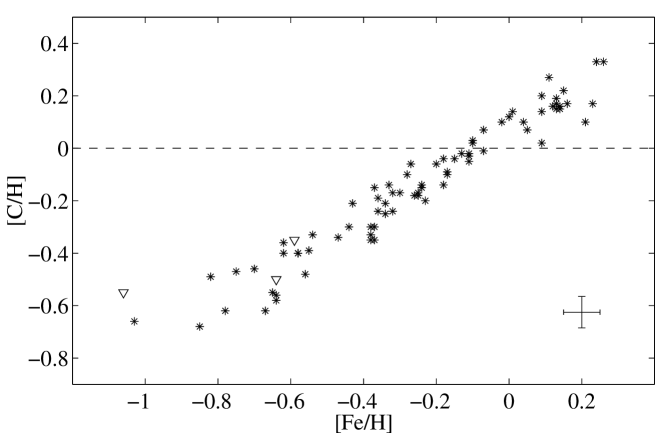
Figure 3: $\mathrm{[C/H]}$ as a function of $\mathrm{[Fe/H]}$. The triangles denote upper limits in $\mathrm{[C/H]}$ and will be excluded in the analysis. A typical error bar is shown in the lower right corner

In Fig. 4a, we have plotted the $\mathrm{[C/Fe]}$ ratios for the observed stars as a function of $\mathrm{[Fe/H]}$. There is a well defined relation with a small scatter around it:

$$\mathrm{[C/Fe]}=(-0.17\pm 0.03)\times\mathrm{[Fe/H]}+(0.065\pm 0.008).$$ (3)

The standard deviation is $0.06$ which again is consistent with the estimated random errors in carbon and iron abundances. Also in this case the effects on the slope from possible systematic errors in $\log g$ are minute.

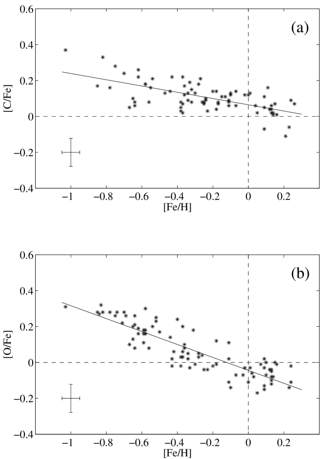
Figure 4: a $\mathrm{[C/Fe]}$ as a function of $\mathrm{[Fe/H]}$. The asterisks denote abundances of observed stars and the full line is the determined slope given in Eq. 3. b $\mathrm{[O/Fe]}$ as a function of $\mathrm{[Fe/H]}$ with data taken from Edvardsson et al. (1993). The slope calculated from this data is given in Eq. 4. Typical error bars are shown in the lower left corners

The small scatter around the linear relations discussed here indicates that the estimates made above of random errors in the carbon abundances are not underestimated. The slope in the second relation, $-0.17\pm 0.03$ is significantly less steep than that in the relation between [O/Fe] and [Fe/H],

$$\mathrm{[O/Fe]}=(-0.36\pm 0.02)\times\mathrm{[Fe/H]}-(0.044\pm 0.010),$$ (4)

as obtained from the results of EAGLNT and also shown in Fig. 4b. The slopes as such reflect the slowly growing significance of iron-producing supernovae Type ia during the evolution of the Galaxy, as compared with the rapid production of oxygen by Supernovae Type ii (see, e.g., EAGLNT). However, the difference between these two slopes will be the major issue in our discussion.

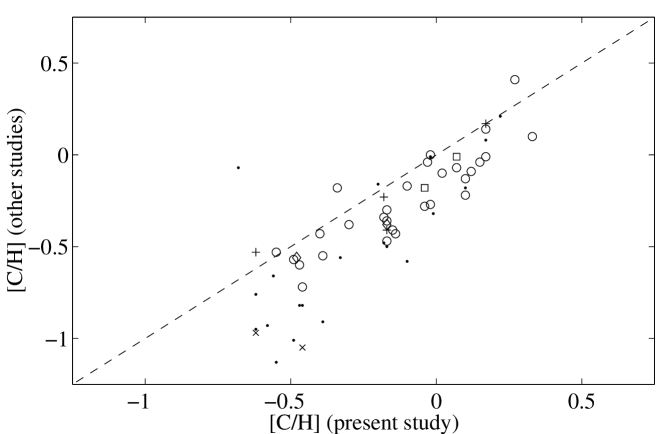
Figure 5: Comparison of derived $\mathrm{[C/H]}$ for the stars in common between earlier studies and present study. Plusses ($+$) are from Clegg et al. (1981), crosses ($\times$) are from Tomkin & Lambert (1984), points ($\cdot$) are from Laird (1985), squares ($\Box$) are from Friel & Boesgaard (1990), diamonds ($\Diamond$) are from Friel & Boesgaard (1992), and open circles ($\circ$) are from Tomkin et al. (1995). The dashed line shows the loci of identical results

Carbon abundances of Galactic Disk stars have been determined by several other groups. We have 20 stars in common with the study of Laird Laird (1985) and 29 in common with Tomkin et al. Tomkin et al. (1995). Furthermore, we have a few stars in common with the studies of Friel & Boesgaard (1990, 1992) and Tomkin & Lambert Tomkin and Lambert (1984) and Clegg et al. Clegg et al. (1981). A comparison between the different results is shown in Fig. 5.

Andersson & Edvardsson Andersson and Edvardsson (1994) found a slope in C/Fe, based on the same line as we have used, however, for fewer stars and lower S/N, of $-0.2$. They also extracted data from previous analyses and separated abundances based on separate features for comparison. The abundances found by Laird Laird (1985) from CH molecular lines show a slope in the $\mathrm{[C/Fe]}$ vs. $\mathrm{[Fe/H]}$ of $-0.10$ if only stars with $\mathrm{[Fe/H]}\geq-1.0$ are considered. The data show considerable scatter, however. Clegg et al. Clegg et al. (1981) found a mean slope of $\approx-0.16\pm 0.08$ from highly excited C i lines, the [C i] $8727\mbox{{\AA}}$ line and CH lines in F and G main-sequence stars. Their data demonstrate systematic differences between results from the different lines used: The highly excited C i and the [C i] $8727\mbox{{\AA}}$ line give a slope of $-0.18$ and the CH-based abundances give $-0.27$, while a slope of $0.00$ was obtained from C₂ lines. Friel & Boesgaard (1990, 1992) show from highly excited C i lines in field stars a slope of $-0.18$, while , more recently, Tomkin et al. Tomkin et al. (1995) derived from the C i line at $7100\mbox{{\AA}}$ of field disk stars a slope of $-0.28$.

In Fig. 5 we also note a small offset of our data; e.g. relative to those of Tomkin et al. (1995) we tend to obtain $\mathrm{[C/H]}$ ratios greater by $0.1\leavevmode\nobreak\ \mbox{dex}$. This may be due to the use of different carbon lines. If our results were true they also indicate a tendency for the Sun to be somewhat carbon poor or iron rich (cf. also Fig. 3). This latter circumstance should be compared with the possible tendency for the Sun to be somewhat poor also in other elements like Mg, Al and Si relative to Fe (Gustafsson 1998). In view of the possible systematic errors involved, e.g., in the gravity scale, we do not consider our offsets from the identity line in Fig. 5 and our finding for the solar type stars to have non-solar $\mathrm{[C/Fe]}$ ratios to be very significant. This, however, deserves further study. Our data show a smaller spread in the $\mathrm{[C/Fe]}$ vs. $\mathrm{[Fe/H]}$ relation than do the other studies. We ascribe this to the high quality of our data, and the insensitivity of the $8727\mbox{{\AA}}$ [C i] line to temperature.

7 Discussion

7.1 Possible sources of carbon

As was mentioned in the Introduction a number of different production sites have been suggested for carbon: supernovae, novae, Wolf Rayet stars, intermediate and low mass stars in connection with the planetary-nebulae stages or even before by superwinds at the end of the red-giant phase. Here, we shall discuss these different possibilities in the light of our observations.

If carbon were produced essentially by SNe ii, with yields relatively independent of the initial metal abundances of the massive stars from which the supernovae originate as is the case for oxygen, then one would expect the slope in the two relations in Fig. 4 to be the same. This is because the yield of carbon produced by a generation of massive stars would scale with that of oxygen. True enough, the $\mathrm{C/O}$ ratios of the nuclei produced and expelled by SNe ii of different mass may be different. E.g., from the tables of Nomoto et al. Nomoto et al. (1997) we find ${}^{12}\mathrm{C}/^{16}\mathrm{O}$ ratios varying from $0.23$ (at $15\mathcal{M}_{\odot}$), $0.21$ ($18\mathcal{M}_{\odot}$), $0.049$ ($25\mathcal{M}_{\odot}$) and $0.016$ ($40\mathcal{M}_{\odot}$). An analogous trend is found from the grid of supernovae models of Woosley & Weaver Woosley and Weaver (1995) (henceforth referred to as WW95) although their $\mathrm{C/O}$ ratios are greater, reflecting their lower rates for the critical $\mathrm{{}^{12}C(\alpha,\gamma)^{16}O}$ reaction. However, the time scale difference between stars in the lower end of the mass interval that produce SNe ii and stars of very great masses is still much smaller than the characteristic time scale for SNe ia, producing iron. Therefore, these different yields of supernovae of different mass are not expected to lead to any significant slope differences in Fig. 4. If the $\mathrm{C/O}$ ratios were dependent on the initial metallicity of the star evolving to a supernova this would, however, lead to a difference. In effect, if the most metal-poor stars would produce relatively more oxygen one could at least qualitatively reproduce the slopes in Fig. 4. However, the SN ii models with different metallicity do not predict any substantial differences in the $\mathrm{C/O}$ ratios of the yields. E.g., the models with solar initial abundances of WW95 have yields with $\mathrm{O/C}=7.1$, when integrated with a mass distribution corresponding to a Salpeter IMF, while those for 1/100 solar metallicity lead to $\mathrm{O/C}=6.6$. Also note that the absolute amount of carbon produced in the models mentioned, as compared with other SN ii products, e.g., Mg, is not sufficient to explain the abundance difference of a factor of 10 found, e.g. in the Sun, cf. WW95 and Thielemann et al. Thielemann et al. (1996). Although there are uncertainties still in predicted carbon yields for SNe ii due to the uncertainty in the $\mathrm{{}^{12}C(\alpha,\gamma)^{16}O}$ rate and the details in the treatment of convection, cf. WW95, the uncertainties do not seem large enough to admit an increase of the carbon yields by a factor of 5. Obviously, another source of carbon is needed.

Supernovae of Type ia, believed to produce most of the iron, do not contribute significant amounts of carbon. E.g., the various models listed by Nomoto et al. Nomoto et al. (1997) give carbon yields smaller than 10% of their iron yields.

Novae may also be ruled out as important sites for the production of carbon since the frequency of such events and their mass loss are too low to enrich the interstellar medium enough with common elements such as ${}^{12}\mathrm{C}$ (Gehrz et al. 1998).

Massive stars may, however, contribute processed material in earlier phases, due to their massive radiation-driven winds. These winds may then contain He and C due to hydrogen and helium burning, but only smaller amounts of O and heavier elements. Maeder Maeder (1992) suggested yields from stars more massive than $25\mathcal{M}_{\odot}$ to be strongly dependent on metallicity, reflecting the fact that more metal rich gas has a much greater cross section for radiation in the ultraviolet. E.g., a $40\mathcal{M}_{\odot}$ solar composition model is suggested to eject about 10% of its mass as He and 10% as C into the interstellar medium, while a corresponding model with 1/20 of the solar metallicity hardly looses anything. These calculations have been detailed by Portinari et al. Portinari et al. (1998) who also produce results for intermediate metallicities. In their models, $\mathrm{C/O}$ of the winds is less than solar for initial masses in the interval $12$ - $30\mathcal{M}_{\odot}$. Not until the mass is on the order of $40\mathcal{M}_{\odot}$ or greater does $\mathrm{C/O}$ become greater than one. Although there is a general agreement between observed and predicted relations for $\mathrm{[C/Fe]}$ vs. $\mathrm{[Fe/H]}$ and $\mathrm{[O/Fe]}$ vs. $\mathrm{[Fe/H]}$, the fit is not perfect. E.g., for carbon a bump with high carbon abundances is predicted around $\mathrm{[Fe/H]}=-0.5$, with a steep slope down in $\mathrm{[C/Fe]}$ when proceeding towards solar $\mathrm{[Fe/H]}$. This is not seen in our observations. On these grounds, however, the origin of carbon in massive stars may certainly not be refuted. The substantial uncertainties in calculated yields, both from supernovae and the massive winds in earlier stages of massive stars, may well explain these deviations from observations.

A more empirical estimate verifies the role that massive stars may play through their winds. The number of WR stars within $3\mbox{kpc}$ from the Sun, a volume for which the sample is thought to be complete, is about 60 (Conti 1988). Of these, about half are WC stars which then implies a number of WC stars in the Galaxy on the order of 300. Typical mass-loss rates from WC stars are $7\cdot 10^{-5}\,\mathcal{M}_{\odot}$/year and $\mathrm{C/He}$ mass ratios range in the interval $0.5$ - $3.3$ (de Freitas & Machado 1988). This implies a total annual carbon contribution to the ISM from the WC stars of about $0.01\mathcal{M}_{\odot}$, which is a very considerable number. In model calculations to be described below, we find a value fairly consistent with that, considering the uncertainties: with the yields of Portinari et al. Portinari et al. (1998) we obtain a total carbon contribution from massive stellar winds of $0.0035\mathcal{M}_{\odot}$ per year, for a star formation rate of $1\mathcal{M}_{\odot}$ per year in the Galaxy, and a Salpeter IMF.

Stars of intermediate and low masses ($<10\mathcal{M}_{\odot}$) may also be significant contributors of carbon on the galactic scale, as was suggested by Tinsley Tinsley (1978), Sarmiento & Peimbert Sarmiento and Peimbert (1985) and Timmes et al. Timmes et al. (1995). The basic argument for these authors was that the estimated contribution from supernovae and novae was not enough to account for the observed carbon abundance. The theoretical yields of carbon from intermediate and low mass stars are, however, highly uncertain, not the least for the numerous low-mass stars. The pioneering calculation of yields by Renzini & Voli Renzini and Voli (1981) were not successful in predicting observed $\mathrm{C/O}$ and $\mathrm{N/O}$ ratios for stars and planetary nebulae, nor could they reproduce the carbon stars of relatively low luminosities in the Magellanic clouds (cf. Note added in proofs by these authors). These calculations are now surpassed by those of Marigo et al. (1996, 1998) who have published yields based on semi-analytical models of AGB stars with mass loss, with several free parameters to describe dredge-up of processed material. They find significant contributions of carbon from stars in the mass interval $1.5$ - $4\mathcal{M}_{\odot}$. Forestini & Charbonnel Forestini and Charbonnel (1997) have calculated evolutionary models to the tip of the AGB with pulsations included and found significant contributions of carbon for the lowest masses, amounting to a few percent of a solar mass for stars around $2$ - $2.5\mathcal{M}_{\odot}$. Both these papers suggest greater yields of carbon for low metallicities (Fig. 9). Empirically, the finding that 50% of the planetary nebulae are carbon rich (with $\mathrm{C/O}\geq 1$), (Zuckerman & Aller 1986; Rola & Stasinska 1994) and a PN birth rate of 1 per year in the Galaxy (Pottasch 1992) and a PN mass of $0.3\mathcal{M}_{\odot}$, suggests a carbon contribution of about $0.003\mathcal{M}_{\odot}$ per year to the ISM. With such a contribution, the PNe could be a major source of carbon. One may ask whether mass loss from carbon stars, i.e. before the PN stage, also could be a major source. Adopting typical mass-loss rates (see Olofsson et al. 1993, 1996; Jura & Kleinmann 1989), $\mathrm{C/O}$ ratios (Lambert et al. 1986) and carbon-star frequencies we find a total carbon contribution of $2\cdot 10^{-4}$ $\mathcal{M}_{\odot}/\mathrm{year}$, which should not be very significant in the global carbon budget of the Galaxy. We note also that Prantzos et al. Prantzos et al. (1994), argue that the time scale for the halo phase of about $1$ - $2\leavevmode\nobreak\ \mbox{Gyrs}$ admits the contribution of carbon by intermediate mass stars to the initial abundance of the Galactic Disk, as predicted from the yields of Renzini & Voli Renzini and Voli (1981), but that the lack of a peak in the $\mathrm{C/O}$ ratio around $\mathrm{[Fe/H]}=-1.0$ suggests other production sites. They conclude from their model calculations that an origin in massive winds as suggested by Maeder Maeder (1992) is most probable.

7.2 Tests of possible carbon sources

One may now ask which of the two major remaining carbon sources – massive stars through massive stellar winds, presumably in the Wolf Rayet WC stage, or the contribution from intermediate/low mass stars through planetary nebulae – is the most significant source. These two different sources could reveal themselves in different strengths of the correlations between carbon abundance and metallicity, and age, respectively. The WC origin of carbon should be expected to lead to a stronger correlation of the carbon abundance with metallicity, while if the age is the dominating factor, determining the carbon abundance as in the planetary nebulae case, one would expect a stronger correlation between $\mathrm{[C/H]}$ and age.

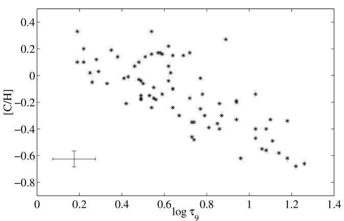
Figure 6: $\mathrm{[C/H]}$ as a function of $\log\tau_{9}$. The scatter in this relation is much greater than in the $\mathrm{[C/H]}$ vs. $\mathrm{[Fe/H]}$ relation (Fig. 3), partly due to errors in the age estimates

In contrast to the strong correlation between the carbon abundance and metallicity, as illustrated in Fig. 3, a much greater scatter is found in the $\mathrm{[C/H]}$ vs. stellar age relation (Fig. 6). A similarly great scatter is found in the [Fe/H]-age diagramme (see EAGLNT, their Fig. 14a). This could indicate a cosmic spread in [Fe/H] at a given age, which then indicates that $\mathrm{[C/H]}$ is more tightly related to metallicity than to age. Another possibility is that the scatter in Fig. 6 is due to random errors in age. If so, these errors must be as large as $0.2\leavevmode\nobreak\ \mbox{dex}$ or around 60%. The estimated errors in the ages are more likely on the order of 25%. Therefore, it seems likely that there is a real spread in the metallicity-age relation and that the primary dependence is on metallicity. This argument is weakened, however, by the possibility that the spread in the $\mathrm{[Fe/H]-age}$ relation is due to the diffusion of stars formed at different distances from the Galactic centre into orbits close to the solar one (Wielen et al. 1996).

We here suggest another test, built on the following argument: If carbon is produced in massive stars, but with metal-abundance dependent yields due to the radiatively driven winds, one would expect a gradual increase of the $\mathrm{C/O}$ ratio with $\mathrm{[Fe/H]}$. This is also observed in the Disk, (Fig. 7). Similarly, if less massive stars produce carbon and expel it as PNe, one again expects a gradual increase of $\mathrm{C/O}$ in the Disk, reflecting the difference in time scale between the carbon producing stars and the massive stars producing oxygen.

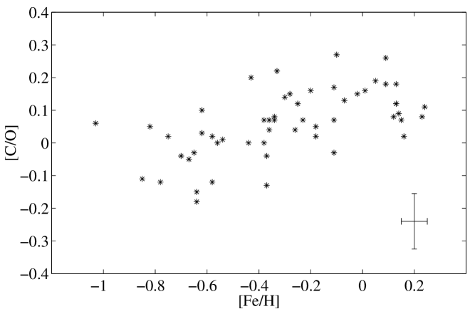
Figure 7: $\mathrm{[C/O]}$ as a function of $\mathrm{[Fe/H]}$. We can see a gradual increase in $\mathrm{[C/O]}$ with $\mathrm{[Fe/H]}$. This observed enhancement of carbon to the ISM could be a result of carbon production in massive stars with metallicity dependent yields or intermediate- and low-mass stars, or possibly a mixture

Our test is built on the fact that these two factors behind the $\mathrm{C/O}$ increase – metallicity and time-scale – are interrelated in different ways in different galaxies. Thus, irregular galaxies, like the Magellanic Clouds, have a lower metallicity ($\mathrm{[Fe/H]_{irr}}$), while the time scale for a more or less continuous star formation history may be of the same order of magnitude as for the Galactic Disk. For these irregulars we therefore expect the massive star contribution of carbon relative to oxygen to be be comparable to that from massive stars in the Disk, when its metal-abundance was $\mathrm{[Fe/H]_{irr}}$. Thus the same slope should be delineated in the $\mathrm{[C/O]}$-$\mathrm{[Fe/H]}$ diagram by the irregulars and the Galactic Disk stars. For the contribution of carbon from intermediate- and low-mass stars, however, we expect a smaller contribution in the Disk when the metal abundance was $\mathrm{[Fe/H]_{irr}}$ if the latter is small enough ($\leq-0.5$), since time then had still not admitted these stars to contribute much. In the more slowly evolving irregulars, however, these contributions are fully developed. Thus, we predict a greater slope in the $\mathrm{[C/O]}$-$\mathrm{[Fe/H]}$ diagramme for the Galactic Disk stars if intermediate- and low-mass stars are more significant as carbon sources.

It should be noted that Edmunds & Pagel Edmunds and Pagel (1978) pointed out that, provided that nitrogen would be formed as a primary element in low-mass stars, the N/O-O/H diagramme could be used for dating galaxy populations. Here, we use a similar idea, for another purpose.

7.3 Models of carbon synthesis in galaxies

We shall now illustrate our discussion by using models of Galactic chemical evolution. Such models must, however, be used with care – in particular when compared quantitatively to real observations – since they are marred by the uncertainties in the in-going data, in particular in yields. Also, the uncertainties in the basic assumptions made in the models are significant. This is illustrated in Fig. 3 of Carigi Carigi (1994) where a number of different models from the literature are intercompared.

Our chemical evolution model is based on the analytical model of the local outer Disk, developed by Pagel & Tautvaišienė Pagel and Tautvaisiene (1995). This model uses the inflow formalism of Clayton Clayton (1985) and the delayed production approximation introduced by Pagel Pagel (1989).

The differential equations describing the chemical evolution are:

$$\frac{\mathrm{d}Z_{1}}{\mathrm{d}u}+\frac{F}{\omega g}Z_{1}=y_{1}(Z(u))$$ (5)

$$\frac{\mathrm{d}Z_{2}}{\mathrm{d}u}+\frac{F}{\omega g}Z_{2}=0\qquad\qquad\mathrm{if}u<\omega\Delta;$$ (6)

$$\frac{\mathrm{d}Z_{2}}{\mathrm{d}u}+\frac{F}{\omega g}Z_{2}=y_{2}(Z(u))\frac{g(u-\omega\Delta)}{g(u)}\qquad\mathrm{if}u\geq\omega\Delta,$$ (7)

where the total mass fraction of a species, $Z_{i}=Z_{1}+Z_{2}$, is the sum of the mass fractions from instantaneous and delayed production. Here, $Z$ is the overall metallicity (per mass). The time-like integration variable $u$, is defined as

$$u\equiv\int_{0}^{t}\omega(t^{\prime})\mathrm{d}t^{\prime},$$ (8)

where $\omega$ ($=0.3\leavevmode\nobreak\ \mbox{Gyr${}^{-1}$}$) is the transition probability for gas to change into stars in unit time at time $t$. The function describing the inflow is of the form

$$\frac{F}{\omega g}=\frac{k}{u+u_{0}}$$ (9)

and can be chosen to be switched on at a specific time $u_{1}$. $F$ is the mass inflow rate, while the parameters $k$ and $u_{0}$ are choosen to fix the ratio of final to initial mass of the system. In this model, $u_{1}=0.14$, $k=3$ and $u_{0}=1.3$, as in Pagel & Tautvaišienė Pagel and Tautvaisiene (1995). Note that before the inflow begins, the second term on the left hand side of Eqs. 5, 6 and 7 is identically zero.

Eventually, the evolution of the gas mass, $g(u)$, is given by

$$\frac{dg}{du}+g=\frac{F}{\omega}.$$ (10)

All parameter values describing the chemical evolution are the same as those chosen by Pagel & Tautvaišienė except for their choice of constant net yields. We explore the effects of metallicity dependent yields $p_{\mathrm{iM}}(Z(u))$, where $Z(u)$ is the overall metallicity. The net yields ($y_{\mathrm{i}}$ in Eqs. 5 and 7) are mass-integrated stellar yields divided by the lock-up fraction, which is treated in the instantaneous recycling approximation.

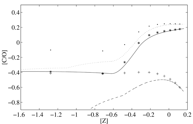
Figure 8: Synthetic $\mathrm{[C/O]}$ ratio of the local disk and dwarf irregular galaxies derived from a chemical evolution model using metallicity dependent yields (Portinari et al. 1998). The full line shows the $\mathrm{[C/O]}$ ratio of the Galactic Disk with carbon produced by high mass stars, the dashed line shows the Disk with products from intermediate and low mass stars, the dotted line is the combined $\mathrm{[C/O]}$ ratio with carbon from high, intermediate and low mass stars in the Disk. The asterisks ($\ast$) represent dwarf irregular galaxy models with carbon from high mass stars, the plusses ($+$) are dwarf irregular galaxies with carbon from intermediate and low mass stars and the points ($\cdot$) represent dwarf irregular galaxies with carbon produced by high, intermediate and low mass stars. The sharp upturn in $\mathrm{[C/O]}$ at $[Z]=-0.6$ is a result of the highly increasing theoretical carbon yield of high mass stars with increasing metallicity

We have used carbon and oxygen yields of Portinari et al. Portinari et al. (1998) for high mass stars and carbon yields of Marigo et al. (1996, 1998) and Forestini & Charbonnel Forestini and Charbonnel (1997) for intermediate and low mass stars. With an adopted linear time-metallicity relation normalized to the solar value, i.e. $Z=0.0055u$, we can calculate the evolution of the $\mathrm{[C/O]}$ ratio with $Z$ (Fig. 8). Oxygen was assumed to be recycled instantaneously while carbon was divided into an instantaneous part (representing carbon production by high-mass stars) and several delayed production parts with different time delays $\omega\Delta$, from $\omega\Delta=0.015$ to $\omega\Delta=1.000$, corresponding to carbon production by stars with masses from $6$ - $9M_{\odot}$ to $1$ - $2M_{\odot}$.

The dwarf irregulars were simulated like local Disk systems (i.e. same parameters as the Disk), however, with different slopes of the time-metallicity relation in order to mimic the slower metal production of heavy elements leading to a lower present metallicity. All systems were evolved for $15\leavevmode\nobreak\ \mbox{Gyrs}$ ($u=4.5$) and thereafter the $\mathrm{[C/O]}$ ratio was read off for comparison with observations.

The results of the simulations are shown in Fig. 8. It is seen that the $\mathrm{C/O}$ ratio for the Galactic Disk, if the carbon is produced by massive stars, shows a gradual and rather steep increase with Disk star metallicities, reflecting the metal-abundance sensitivity of the radiatively driven winds. The models representing dwarf irregulars line up nicely along the Disk curve. When carbon production from intermediate and low mass stars is added, the dwarf irregulars are elevated above the $\mathrm{C/O}$ ratios of the Disk, in particular for the low metallicity systems. Thus, in this case the dwarf irregulars should delineate a relation with smaller slope in the diagramme, as was argued on qualitative grounds above. In the extreme case (lower part of the figure) when only intermediate- and low-mass stars contribute the slope difference is very pronounced.

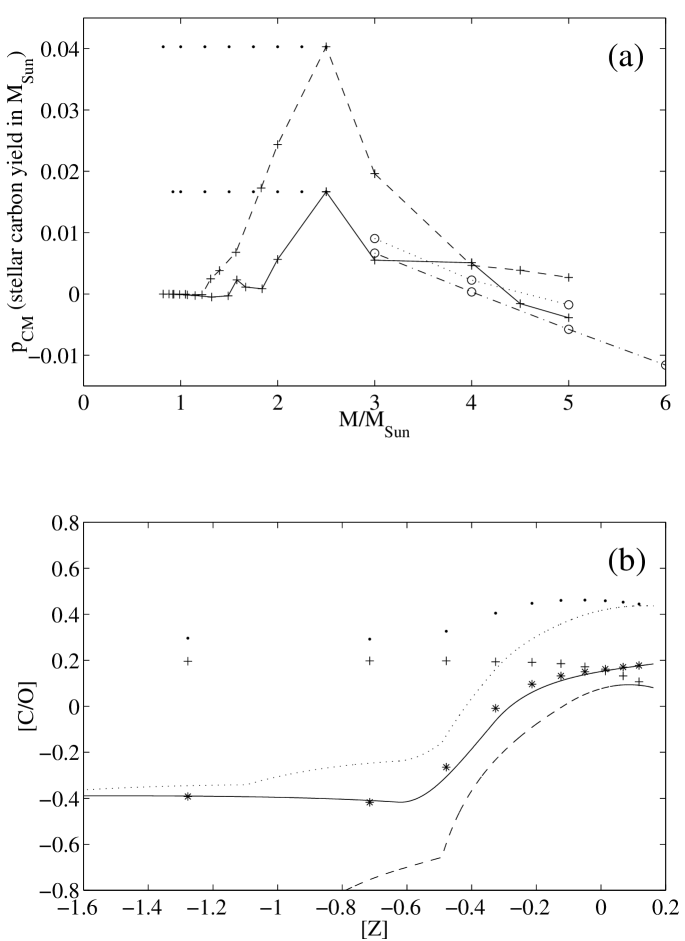
Figure 9: a Theoretical stellar carbon yields (in $\mathcal{M}_{\odot}$) for intermediate and low mass stars. The full line is the yield at $Z=0.02$ and the dashed line is the yield at $Z=0.008$ from Marigo et al. (1996, 1998). The dash-dotted and the dotted lines show the yield at $Z=0.02$ and $Z=0.005$ respectively, calculated by Forestini & Charbonnel (1997). Alternative increased carbon yields for low mass stars ($0.95$ - $2.5\mathcal{M}_{\odot}$) are indicated as dotted horizontal lines. b Synthetic $\mathrm{[C/O]}$ ratios in the Galactic Disk with the increased carbon yields for low mass stars. Symbols as in Fig. 8

Since the relative contribution to the production of carbon of stars of different masses is highly uncertain we have ad hoc increased the yields of Marigo et al. for the stars with masses below $2.5\mathcal{M}_{\odot}$ according to Fig. 9a. Such a change will guarantee that the frequency of planetary nebulae with $\mathrm{C/O}\geq 1$ gets as high (or even higer) than observed, and that the absolute amount of carbon produced is as high as observed. This is illustrated in Fig. 9b. Again we notice the very pronounced slope difference between the Disk star relation and that of dwarf irregulars.

7.4 Results of the tests

Before we discuss the results of the test it should be noted that our observations of stars in the Solar neighbourhood may not map the chemical evolution all the way back to the time of formation of the Disk. Short lived intermediate-mass stars could have enriched the ISM, provided that they are sites of high carbon production. This is in clear contradiction, though, to the theoretical yield calculations (Fig. 9a) which indicate that the intermediate-mass stars in the upper mass region do not produce carbon in large amounts. They are also less numerous in comparison to stars of lower mass which further limits their relative contribution to the ISM. Moreover, if intermediate-mass stars were the main origin of carbon in the Disk in general, the carbon yield has to be metal dependent as for the massive stars, again in contradiction to the theoretical yields which rather decrease with increasing metallicity. However, the yields are uncertain and observationally, we are not able to exclude them as carbon producers of some importance.

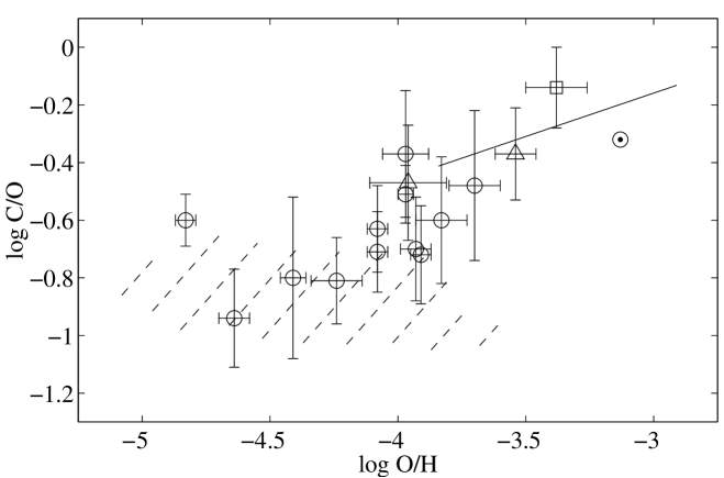
Figure 10: Observed $\mathrm{C/O}$ ratios in various metal-poor galaxies. Open circles ($\circ$) represent data for H ii regions in different galaxies from Kobulnicky & Skillman (1998) and references therein, the square ($\Box$) is the mean $\log\mathrm{C/O}$ ratio calculated from several observations of the Orion nebula. The triangles ($\triangle$) are $\mathrm{C/O}$ ratios deduced from supergiant stars in LMC and SMC by Hill et al. (1995, 1997). The full line indicates the calculated slope of the Galactic Disk stars, derived from observed carbon and oxygen abundances. The hatched area in the lower part of the figure indicates the location of halo dwarf stars, studied by Tomkin et al. (1992). The location in the horizontal direction of these stars is relatively uncertain due to temperature uncertainties. The Sun is also indicated in the figure as a $\odot$. The slope of the Disk stars is not steeper than the slope of the dwarf irregulars, indicating that low-mass stars are not significant carbon contributors relative to metal-rich high-mass stars. The role of the short lived intermediate-mass stars should be further investigated

In order to carry out the test empirically we first use the observations of massive supergiants in the Magellanic Clouds. The determinations for supergiants in the SMC (Hill et al. 1997) and LMC (Hill et al. 1995) are plotted in Fig. 10. The relation for the Disk stars was obtained by combining Eqs. 3 and 4. From this we find that the stars in the Magellanic Clouds seem to take positions in the diagramme characteristic of the Galactic Disk stars which does not support the hypothesis of C being made in intermediate- or low-mass stars. However, the supergiant CNO abundances may be affected by dredge-up of CNO processed material, which makes the value of this test uncertain.

In Fig. 10 we have also plotted the location of H ii regions in various metal-poor galaxies according to Kobulnicky & Skillman Kobulnicky and Skillman (1998) and references therein and the locus of halo dwarf stars according to Tomkin et al. Tomkin et al. (1992). There seems to be a tendency for the halo stars to have low C/O ratios as compared with Disk stars. This may, however, be due to systematic errors is the analysis of the halo stars, or possibly of the Disk stars (the latter is suggested by the deviating position of the sun in Fig. 10), but the suggested tendency is worth further investigation.

In Fig. 10 we find the galaxies to define a slope that seems as steep or even steeper than that of the Galactic Disk stars. Although adopting an [O/Fe] slope of $-0.40$ (cf. Eq. 4 and Fig. 4b) the picture does not alter significantly. Actually, if we drop the mathematically derived equations (Eqs. 3 and 4), a somewhat higher value of both the [O/Fe]- and [C/Fe] slope may be argued for just by inspecting Fig. 4 by eye. The C/O slope would then again decrease towards the adopted value (Fig. 10). Even if the slope of the Disk stars is further steepened when the halo stars are added, the locii of the metal-poor galaxies do not seem compatible with the hypothesis that carbon has been formed mainly in stars of lower mass. The most direct conclusion from this would thus be that the production of carbon occurs at a time-scale characteristic of high-mass or possibly intermediate-mass stars of relatively high mass, but that the yields are metal-abundance dependent, just as is expected from massive stellar radiatively driven winds, e.g. from WC stars.

There may be several arguments against a test of this character. One may be the possibility that carbon, and oxygen as well as iron, could be severely depleted by grain formation in the interstellar medium of the irregular galaxies. A depletion independent of metallicity for carbon, but increasing with metallicity for oxygen, seems possible and would qualitatively lead to the effect observed. It is, however, questionable whether this effect could be as great as required to explain the full effect or to fully compensate for the effect due to carbon formation by low-mass stars.

Another possibility may be that the remnants from the oxygen producing SNe are lost from the irregulars, and more so later in their evolution when the gas density in the galaxy and its surroundings is less, while the slower carbon-rich winds from the PNe are mostly retained. This would, however, diminish the slope of the irregulars in the diagramme, which would then strengthen our arguments for the high-mass stars as main contributors of carbon.

The dwarf irregular galaxies could be systems of much smaller age than the Galactic Disk. E.g., even if Garnett et al. Garnett et al. (1997) have pointed out that a population of stars older than the present star burst is probable in I Zw 18, the mean age of stars in this system could still be much younger than the Galactic Disk. However, at least in the Large Magellanic Cloud there is strong evidence for a dominating population of an age comparable to that of the Galactic Disk (Ardeberg et al. 1997).

Finally, if the main source of carbon is high-mass stars one has to explain why planetary nebulae, found above to provide as much as $0.003\mathcal{M}_{\odot}$ of carbon per year to the Galaxy today, do not constitute a major carbon source. The statistics of PNe must comprize low-mass stars ($\leq 2\mathcal{M}_{\odot}$) as a major group; in view of the great PN birth rate. Therefore, if the masses, the birth rate or the carbon abundances of the PNe are not seriously overestimated, one has to advocate metal-abundance sensitive yields for these, such that the amount of carbon produced be greater the higher the metal-abundance. This is contrary to the tendency found in model calculations both by Marigo et al. (1996, 1998) and by Forestini & Charbonnel Forestini and Charbonnel (1997).

8 Conclusions

We have determined accurate carbon abundances for a set of 80 Galactic Disk stars. We find the resulting $\mathrm{[C/H]}$ values to correlate very well with the iron abundances $\mathrm{[Fe/H]}$, with a slope, however, that is smaller than unity such that $\mathrm{\Delta[C/Fe]/\Delta[Fe/H]}=-0.17\pm 0.03$. From this, and the corresponding variation of $\mathrm{[C/O]}$, we conclude by comparing to dwarf irregular galaxies of different metallicity that carbon is predominantly produced in the Galactic Disk by massive stars, ejecting carbon in radiatively driven massive winds, in particular during their Wolf Rayet stage. Estimates of yields from massive stars support this conclusion, even if yields from intermediate- and low-mass stars also suggest those to be of some significance as sources of carbon. A particular problem is raised by the estimates that about half the planetary nebulae may be carbon rich (with $\mathrm{C/O}\geq 1$); if so one has to explain where this excess carbon has gone. In particular, why is it not visible as a steeper slope for the Disk stars than for the dwarf galaxies in the $\mathrm{[C/O]}$ – $\mathrm{[O/H]}$ diagramme?

The systematic study of carbon abundances of WR stars, carbon stars and planetary nebulae of different progenitor mass and metallicity in the Galaxy and neighbouring galaxies should be persued, in order to establish more reliable empirical yields for high-, intermediate- and low-mass stars. These abundances should also be related to the abundances of nitrogen and the s elements which are thought to be formed in intermediate- and low-mass stars. A test similar to that applied here with metal-poor galaxies should be possible and rewarding by using radial gradients in C/O and O/H measured for disk galaxies. Also, isotopic characteristics of WR stars in solar-system material, e.g. as presolar grains in meteorites, should be further looked for. At present that situation is not clear; according to the recent review by Arnould et al. (1997) there is to date no clear and unambiguous signature of the existence in meteorites of presolar grains of WR origin identified in the laboratory, while grains of AGB star origin have most probably been identified (Anders & Zinner 1993).