The geometry of second–order statistics – biases in common estimators

Abstract

Second–order measures, such as the two–point correlation function, are geometrical quantities describing the clustering properties of a point distribution. In this article well–known estimators for the correlation integral are reviewed and their relation to geometrical estimators for the two–point correlation function is put forward. Simulations illustrate the range of applicability of these estimators. The interpretation of the two–point correlation function as the excess of clustering with respect to Poisson distributed points has led to biases in common estimators. Comparing with the approximately unbiased geometrical estimators, we show how biases enter the estimators introduced by ?, ?, and ?. We give recommendations for the application of the estimators, including details of the numerical implementation. The properties of the estimators of the correlation integral are illustrated in an application to a sample of IRAS galaxies. It is found that, due to the limitations of current galaxy catalogues in number and depth, no reliable determination of the correlation integral on large scales is possible. In the sample of IRAS galaxies considered, several estimators using different finite–size corrections yield different results on scales larger than 20$h^{-1}$Mpc, while all of them agree on smaller scales.

1 Introduction

Second–order measures, also called two–point measures, are still one of the major tools to characterize the spatial distribution of galaxies and clusters. Probably the best known are the two–point correlation function $g(r)$ and the normed cumulant $\xi_{2}(r)=g(r)-1$ (e.g. ?). With the mean number density denoted by $\overline{\rho}$,

$$\overline{\rho}^{2}g(r)\ {\rm d}V({\mathbf{x}}_{1}){\rm d}V({\mathbf{x}}_{2})$$ (1)

describes the probability to find a point in the volume element ${\rm d}V({\mathbf{x}}_{1})$ and another point in ${\rm d}V({\mathbf{x}}_{2})$, at the distance $r=\|{\mathbf{x}}_{1}-{\mathbf{x}}_{2}\|$, $\|\cdot\|$ is the Euclidean norm of a vector. The correlation integral $C(r)$ (e.g. ?) is the average number of points inside a ball of radius $r$ centred on a point of the distribution; hence,

$$C(r)=\int_{0}^{r}{\rm d}s\ \overline{\rho}\ 4\pi s^{2}g(s).$$ (2)

In Appendix A we discuss other common two–point measures.

The correlation integral $C(r)$ and the two–point correlation function $g(r)$ are defined as ensemble averages. If we want to estimate $C(r)$ from one given point set, as provided by the spatial coordinates of galaxies, we have to use volume averages which yield an estimator $\widehat{C}(r)$.

Since all astronomical catalogues are spatially limited, i.e.  the observed galaxies lie inside a spatial domain ${\cal D}$, we must correct for boundary effects. Estimators of the two–point correlation function including finite–size corrections have been proposed by ?, ?, ?, ?, ?, ?, and ?, to name only a few. In a recent paper ? introduced improved estimators of point process statistics, with special emphasis on the accurate estimation of the density $\overline{\rho}$.

An estimator $\widehat{C}(r)$ is called unbiased if the expectation of $\widehat{C}(r)$ equals the true value of $C(r)$:

$${\mathbb{E}}\ [\widehat{C}(r)]=C(r).$$ (3)

${\mathbb{E}}$ denotes the expectation value, the average over realizations of the point process. An estimator is called consistent, if the estimates $\widehat{C}(r)$ obtained inside a finite sample geometry ${\cal D}$ from one space filling realization, converge towards the true value of $C(r)$, as the sample volume $|{\cal D}|$ increases:

$$\widehat{C}(r)\overset{|{\cal D}|\rightarrow\infty}{\longrightarrow}C(r).$$ (4)

We call an estimator ratio–unbiased if it is the quotient of two unbiased quantities. Whether such a quotient gives a reliable estimate must be tested . Often this is only possible with simulations (see Sect. 2.5, see also ?).

For the comparison of a simulated point distribution with an observed galaxy distribution within the same sample geometry and with the same selection effects, unbiasedness (or consistency) is not a major concern. It is more important that the variance of the estimator is small. This may give tighter bounds on the cosmological parameters entering the simulations.

This article is organized as follows. In Sect. 2 we will review several estimators for the correlation integral. With simulations of two drastically different point process models, namely a featureless Poisson process and a highly structured line segment process, the variance and the bias of the estimators are investigated. Closely connected to these estimators for the correlation integral are the geometrical estimators for the two–point correlation function which will be discussed in Sect. 3. Some popular pair–count estimators for the two-point correlation function are considered in Sect. 4. We derive the geometrical properties of the pair–counts. By comparing with the geometrical estimators of Sect. 3 and with numerical examples we show how biases enter. We comment on the improved estimators of ? in Sect. 5. As an application, we investigate the clustering properties of galaxies in a volume limited sample of the IRAS 1.2 Jy redshift catalogue in Sect. 6. We conclude and give recommendation for the application of the estimators in Sect. 8. In the Appendices we summarize currently used two–point measures and discuss some details concerning the numerical implementation of the estimators.

2 Estimators for the correlation integral $C(r)$

Consider a set of points ${\cal X}=\{{\mathbf{x}}_{i}\}_{i=1}^{N}$, ${\mathbf{x}}_{i}\in{\mathbb{R}}^{3}$, supplied by the redshift coordinates of a galaxy or cluster survey. All points ${\mathbf{x}}_{i}$ are inside the sample geometry ${\cal D}$.

2.1 The naïve estimator for $C(r)$

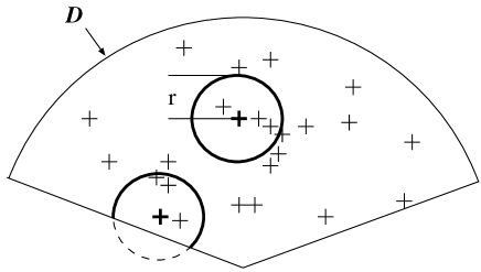
Figure 1: In the naïve estimator $\widehat{C_{0}}(r)$ all points are used as centres for the determination of $N_{i}(r)$. $N_{i}(r)$ is underestimated for points near the boundary of ${\cal D}$.

The naïve and biased estimator of the correlation integral $\widehat{C_{0}}(r)$ is defined by

$$\widehat{C_{0}}(r)=\frac{1}{N}\sum_{i=1}^{N}N_{i}(r),$$ (5)

where

$$N_{i}(r)=\sum_{j=1;j\neq i}^{N}\mbox{1l}_{[0,r]}(\|{\mathbf{x}}_{i}-{\mathbf{x}}_{j}\|)$$ (6)

is the number of points in a sphere with radius $r$ around the point ${\mathbf{x}}_{i}$.

$$\mbox{1l}_{A}(x)=\begin{cases}1&\text{for }x\in A,\\ 0&\text{for }x\notin A\end{cases}$$ (7)

denotes the indicator function of the set $A$. $\widehat{C_{0}}(r)$ is the mean value of $N_{i}(r)$, averaged over all points ${\mathbf{x}}_{i}$. For points ${\mathbf{x}}_{i}$ near the boundary of ${\cal D}$ and for large radii $r$ in particular the number of points $N_{i}(r)$ is underestimated, and $\widehat{C_{0}}(r)$ is biased towards smaller values (see Fig. 1).

2.2 Minus–estimators for $C(r)$

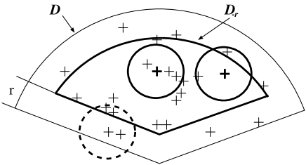
Figure 2: In the minus–estimators only points inside ${\cal D}_{-r}$ are taken into account in the determination of $N_{i}(r)$.

As an obvious restriction, only points, further than $r$ away from the boundary of ${\cal D}$ are used as centres for the calculation of $N_{i}(r)$. Doing so we make sure, that we see all data points inside the sphere of radius $r$ around a point ${\mathbf{x}}_{i}$. ${\cal D}_{-r}$ is the shrunken window (see Fig. 2)

$${\cal D}_{-r}=\{{\mathbf{y}}\in{\cal D}\leavevmode\nobreak\ :\leavevmode\nobreak\ {\cal B}_{r}({\mathbf{y}})\subset{\cal D}\},$$ (8)

where ${\cal B}_{r}({\mathbf{y}})$ denotes a sphere of radius $r$ centred on ${\mathbf{y}}$, and

$$N_{r}=\sum_{i=1}^{N}\mbox{1l}_{{\cal D}_{-r}}({\mathbf{x}}_{i}).$$ (9)

yields the number of points inside ${\cal D}_{-r}$ The minus–estimator $\widehat{C_{1}}(r)$ reads:

$$\widehat{C_{1}}(r)=\frac{1}{N_{r}}\ \sum_{i=1}^{N}\mbox{1l}_{{\cal D}_{-r}}({\mathbf{x}}_{i})\ N_{i}(r)\quad\text{ for }N_{r}>0.$$ (10)

In the case of stationary point processes this estimator is ratio–unbiased (e.g. ?). However, for large radii only a small fraction of the points is included as centres. Therefore, we are limited to scales up to the radius of the largest sphere that lies completely inside the sample geometry. With this estimator we do not have to make any assumption about the distribution of points outside the window ${\cal D}$. This is important for the investigation of inhomogeneous, scale–invariant or “fractal” point distributions. Pietronero and coworkers employed this type of estimator (see Appendix A and ?).

Let us introduce another variant of the minus–estimator, which also does not require any assumption about the missing data outside the sample window ${\cal D}$. An unbiased estimator of the number density is given by

$$\widehat{\rho_{1}}=\frac{N}{|{\cal D}|},$$ (11)

and an alternative ratio–unbiased minus–estimator may be defined by

$$\widehat{C_{2}}(r)=\frac{1}{\widehat{\rho_{1}}\ |{\cal D}_{-r}|}\ \sum_{i=1}^{N}\mbox{1l}_{{\cal D}_{-r}}({\mathbf{x}}_{i})\ N_{i}(r)\quad\text{ for }|{\cal D}_{-r}|>0.$$ (12)

$\widehat{C_{2}}(r)$ differs from $\widehat{C_{1}}(r)$ in that we estimate the number density with $N_{r}/|{\cal D}_{-r}|$ instead of $\widehat{\rho_{1}}$, and an estimate of $\overline{\rho}$ from a larger volume than in $\widehat{C_{1}}(r)$ is used. This may be important, if the galaxy catalogue under consideration is centred on a large cluster. Then $N_{r}\geq|{\cal D}_{-r}|\leavevmode\nobreak\ \widehat{\rho_{1}}$, and therefore $\widehat{C_{1}}(r)$ systematically underestimates the correlation integral $C(r)$. On the other hand, in $\widehat{C_{1}}(r)$ the same points are used for the determination of the numerator and denominator, which empirically yields a reduced variance. In Sect. 2.5 we will see that the large variance of $\widehat{C_{2}}(r)$ makes this estimator rather useless.

2.3 Ripley–estimator for $C(r)$

The Ripley–estimator Ripley (1976) uses all points inside ${\cal D}$ as centres for the counts $N_{i}(r)$ (see Eq. 6). The bias in $\widehat{C_{0}}(r)$ is corrected with weights:

$$\widehat{C_{3}}(r)=\frac{1}{N}\sum_{i=1}^{N}\sum_{j=1;j\neq i}^{N}\mbox{1l}_{[0,r]}(\|{\mathbf{x}}_{i}-{\mathbf{x}}_{j}\|)\times\\ \times\ \omega_{l}({\mathbf{x}}_{i},\|{\mathbf{x}}_{i}-{\mathbf{x}}_{j}\|)\ \omega_{g}(\|{\mathbf{x}}_{i}-{\mathbf{x}}_{j}\|),$$ (13)

with the local pair weight Ripley (1976)

$$\omega_{l}({\mathbf{x}}_{i},s)=\begin{cases}\frac{4\pi s^{2}}{\text{area}(\partial{\cal B}_{s}({\mathbf{x}}_{i})\cap{\cal D})}&\text{for }\partial{\cal B}_{s}({\mathbf{x}}_{i})\cap{\cal D}\neq\emptyset,\\ 0&\text{for }\partial{\cal B}_{s}({\mathbf{x}}_{i})\cap{\cal D}=\emptyset,\end{cases}$$ (14)

inversely proportional to the part of the spherical surface with radius $s$ around the point ${\mathbf{x}}_{1}$ which is inside the survey boundaries (see Fig 3). $\partial{\cal B}_{s}({\mathbf{x}})$ is the surface of the sphere ${\cal B}_{s}({\mathbf{x}}_{i})$ with radius $s$ centred on ${\mathbf{x}}_{i}$. With $\omega_{l}({\mathbf{x}}_{i},s)$ we correct locally for possible points at distance $s$ outside the sample geometry ${\cal D}$.

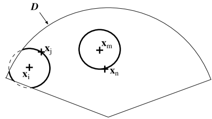
Figure 3: The local weight $\omega_{l}({\mathbf{x}}_{m},s)$ equals unity for the point ${\mathbf{x}}_{m}$ with $s=\|{\mathbf{x}}_{m}-{\mathbf{x}}_{n}\|$. At the point ${\mathbf{x}}_{i}$ with $s=\|{\mathbf{x}}_{i}-{\mathbf{x}}_{j}\|$ the local weight is larger than unity.

The global weight

$$\omega_{g}(s)=\frac{|{\cal D}|}{|\{{\mathbf{z}}\in{\cal D}\leavevmode\nobreak\ |\leavevmode\nobreak\ \partial{\cal B}_{s}({\mathbf{z}})\cap{\cal D}\neq\emptyset\}|},$$ (15)

was introduced by ?. $\omega_{g}(s)$ is inversely proportional to the volume occupied by points ${\mathbf{z}}\in{\cal D}$ for which the surface $\partial{\cal B}_{s}({\mathbf{z}})$ intersects the sample geometry ${\cal D}$ (see Fig. 4).

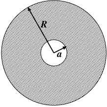
Figure 4: The shaded area marks the set $\{{\mathbf{x}}\in{\cal D}\leavevmode\nobreak\ |\leavevmode\nobreak\ \partial{\cal B}_{s}({\mathbf{x}})\cap{\cal D}\neq\emptyset\}$ for a spherical sample geometry ${\cal D}={\cal B}_{R}$, with $s=R+a$.

In typical sample geometries the global weight $\omega_{g}(s)$ is equal to unity up to fairly large radii $s$. For example, $\omega_{g}(s)$ exceeds unity only for $s>R$ in a spherical sample geometry with radius $R$ (see Fig. 4). For $r<\max\{s\in{\mathbb{R}}^{+}\text{ with }|\{{\mathbf{x}}\in{\cal D}\leavevmode\nobreak\ |\leavevmode\nobreak\ \partial{\cal B}_{s}({\mathbf{x}})\cap{\cal D}\neq\emptyset\}|>0\}$, $\widehat{C_{3}}(r)$ is ratio–unbiased Ohser (1983).

2.4 Ohser and Stoyan estimators for $C(r)$

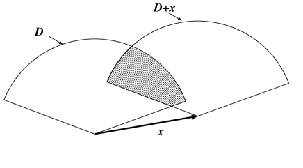
Figure 5: The set–covariance $\gamma_{\cal D}({\mathbf{x}})$ is the volume of the shaded set ${\cal D}\cap{\cal D}+{\mathbf{x}}$.

Another estimator using a weighting strategy of point pairs was proposed by ?:

$$\widehat{C_{4}}(r)=\frac{1}{N}\sum_{i=1}^{N}\sum_{j=1;j\neq i}^{N}\mbox{1l}_{[0,r]}(\|{\mathbf{x}}_{i}-{\mathbf{x}}_{j}\|)\ \frac{|{\cal D}|}{\gamma_{\cal D}({\mathbf{x}}_{i}-{\mathbf{x}}_{j})}\\ \text{if }\gamma_{\cal D}({\mathbf{x}}_{i}-{\mathbf{x}}_{j})>0\text{ for all }\|{\mathbf{x}}_{i}-{\mathbf{x}}_{j}\|<r.$$ (16)

Here the pair–weight is equal to the fraction $|{\cal D}|/\gamma_{\cal D}({\mathbf{x}})$, with the set–covariance (see Fig. 5)

$$\gamma_{\cal D}({\mathbf{x}})=|{\cal D}\cap{\cal D}+{\mathbf{x}}|.$$ (17)

${\cal D}+{\mathbf{x}}$ is the sample geometry shifted by the vector ${\mathbf{x}}$, and $\gamma_{\cal D}({\mathbf{x}})$ is the volume of the intersection of the original sample with the shifted sample. This estimator is ratio–unbiased for stationary point processes; isotropy is not needed in the proof Ohser & Stoyan (1981).

Closely related to the estimator $\widehat{C_{4}}(r)$ is its isotropized counterpart Ohser & Stoyan (1981):

$$\widehat{C_{5}}(r)=\frac{1}{N}\sum_{i=1}^{N}\sum_{j=1;j\neq i}^{N}\mbox{1l}_{[0,r]}(\|{\mathbf{x}}_{i}-{\mathbf{x}}_{j}\|)\ \frac{|{\cal D}|}{\overline{\gamma_{\cal D}}(\|{\mathbf{x}}_{i}-{\mathbf{x}}_{j}\|)},\\ \text{for }\overline{\gamma_{\cal D}}(r)>0,$$ (18)

where $\overline{\gamma_{\cal D}}(r)$ is the isotropized set–covariance:

$$\overline{\gamma_{\cal D}}(r)=\frac{1}{4\pi}\int_{0}^{2\pi}\int_{0}^{\pi}\ \sin(\theta){\rm d}\theta{\rm d}\phi\ \gamma_{\cal D}({\mathbf{x}}(r,\theta,\phi)).$$ (19)

2.5 Comparison of the estimators for $C(r)$

Since the estimators for $C(r)$ considered above are only ratio–unbiased, we have tested whether they give reliable results with two drastically different examples of point processes. This also enables us to compare the variances of the estimators. Several analytical approaches have been put forward to investigate the variance of estimators for two–point measures. The majority of them relies on Poisson or binomial processes (e.g. ?, and ?, see however ?, and ?). A similar numerical comparison of estimators for two–point measures in the two–dimensional case was performed by ?.

Figure 6: A comparison of the estimators $\widehat{C_{0}}(r)$ to $\widehat{C_{5}}(r)$ for a Poisson process with number density $\overline{\rho}=200$ in the unit box. The solid line marks the sample mean, the shaded area is the 1$\sigma$–range estimated from 10,000 realizations, and the dashed line is the true $C_{P}(r)$.

As a simple point process model showing no large–scale structure we study the behaviour of the estimators for a Poisson process with mean number density $\overline{\rho}$. The mean value of the correlation integral is then

$$C_{P}(r)=\overline{\rho}\ \frac{4\pi}{3}r^{3}.$$ (20)

In Fig. 6 a numerical comparison of the estimators $\widehat{C_{0}}(r)$ to $\widehat{C_{5}}(r)$ for a Poisson process with $\overline{\rho}=200$ in the unit cube is shown. The mean and the variance were determined from 10,000 realizations. As expected, a strong bias towards lower values for large $r$ is seen in $\widehat{C_{0}}(r)$; the other estimators do not show any bias. $\widehat{C_{1}}(r)$ is defined only for samples with $N_{r}>0$. Since there were samples with $N_{r}=0$ for $r\geq 0.325$ within the 10,000 realizations of the Poisson process, $\widehat{C_{1}}(r)$ is shown only for radii smaller than $0.325$.

Looking at the absolute errors in Fig. 6, we see that the minus–estimators exhibit larger errors than the others in particular, $\widehat{C_{2}}(r)$ becomes useless on larger scales. The relative errors (the standard error per mean value) exhibit a “shot noise” peak for small $r$ (see Fig. 7). All the estimators using weighting schemes show comparable errors, but especially for large $r$, the Ripley estimator $\widehat{C_{3}}(r)$ gives the smallest errors.

Figure 7: The comparison of the relative errors of the estimators for a poisson process with number density $\overline{\rho}=200$ in the unit box: $\widehat{C_{0}}(r)$ (solid), $\widehat{C_{1}}(r)$ (dotted), $\widehat{C_{2}}(r)$ (short dashed), $\widehat{C_{3}}(r)$ (long dashed), $\widehat{C_{4}}(r)$ (short dashed–dotted, on top of $\widehat{C_{0}}(r)$), $\widehat{C_{5}}(r)$ (long dashed–dotted, on top of $\widehat{C_{0}}(r)$).

Figure 8: A comparison of the estimators with number density $\widehat{C_{0}}(r)$ to $\widehat{C_{5}}(r)$ for a random distribution of points with $\overline{\rho}=200$ on line segments with lenght $l=0.1$ and segment density $\overline{\rho}_{s}=20$ in the unit box. The solid line marks the sample mean, the shaded area is the 1$\sigma$–range estimated from 10,000 realizations, and the dashed line is the true $C_{S}(r)$.

To investigate the performance of the estimators for highly structured and clustered point process models, we study points randomly distributed on line segments which are themselves uniformly distributed in space and direction. From ?, p. 286 (see also ?) we obtain:

$$C_{S}(r)=\begin{cases}\overline{\rho}\ \frac{4\pi}{3}r^{3}+\frac{\overline{\rho}}{\overline{\rho}_{s}}\left(\frac{2r}{l}-\frac{r^{2}}{l^{2}}\right)&\text{ for }r<l\\ \overline{\rho}\ \frac{4\pi}{3}r^{3}+\frac{\overline{\rho}}{\overline{\rho}_{s}}&\text{ for }r\geq l;\\ \end{cases}$$ (21)

$l$ is the length of the line segments and $\overline{\rho}_{s}$ is the mean number density of line segments; $l\overline{\rho}_{s}$, $\overline{\rho}/(l\overline{\rho}_{s})$, $\overline{\rho}$ denote the mean length density, the mean number of points per line segment, and the mean number density in space, respectively. A similar model for the distribution of galaxies is discussed by ?. In Fig. 8 we compare the mean and the variance of the estimators for 10,000 realizations of a line segment process with $\overline{\rho}=200$, $l=0.1$ and $\overline{\rho}_{s}=20$.

As before, $\widehat{C_{0}}(r)$ shows a strong bias on large scales, but also the other estimators include some bias towards smaller values. Some of the random samples showed $N_{r}=0$ for $r<0.175$, therefore $\widehat{C_{1}}(r)$ is given only for smaller radii. Comparing Fig. 8 and Fig. 6 we see that this clustered point distribution leads to a significantly larger variance (see also ?). The relative errors (Fig. 9) on large scales are nearly twice as large as in the case of a Poisson process with the same number density (Fig. 7). Since we are looking at a clustered distribution, the “shot noise” peak is shifted to very small radii, not visible in Fig. 9. Again, the minus–estimator $\widehat{C_{2}}(r)$ becomes unreliable for large $r$. The estimators using weighting schemes display a significantly smaller variance on all scales, whereas the Ripley estimator $\widehat{C_{3}}(r)$ gives the smallest variance on large scales. Simulations with different parameters $l$ and $\overline{\rho_{s}}$ led to the same conclusions.

Figure 9: The comparison of the relative errors of the estimators for a random distribution of points with number density $\overline{\rho}=200$ on line segments with lenght $l=0.1$ and segment density $\overline{\rho}_{s}=20$ in the unit box: $\widehat{C_{0}}(r)$ (solid), $\widehat{C_{1}}(r)$ (dotted), $\widehat{C_{2}}(r)$ (short dashed), $\widehat{C_{3}}(r)$ (long dashed), $\widehat{C_{4}}(r)$ (short dashed–dotted), $\widehat{C_{5}}(r)$ (long dashed–dotted, on top of $\widehat{C_{4}}(r)$).

A possible explanation why $\widehat{C_{3}}(r)$ shows a smaller variance than $\widehat{C_{4}}(r)$ and $\widehat{C_{5}}(r)$ (see Figs. 7 and 9) is that the local weight $\omega_{l}({\mathbf{x}}_{i},s)$ used in $\widehat{C_{3}}(r)$ is larger than unity only for a point ${\mathbf{x}}_{i}$ with another point at distance $s(\leq r)$ and with ${\mathbf{x}}_{i}$ closer to the boundary of the sample than $s$. The weight equals unity for all other point pairs. Contrary, in $\widehat{C_{4}}(r)$ and $\widehat{C_{5}}(r)$ the corresponding weights are larger than unity for all point pairs. Each of these three estimators is ratio–unbiased, hence, correcting for finite size effects, but a frequent use of weights larger than unity increases the variance. ? calculate the weights used in the estimation of the factorial moments minimizing the variance of the factorial moments (see also ?).

3 Geometrical estimators for the two–point correlation function $g(r)$

In contrast to estimators for the correlation integral, all estimators of the two–point correlation function using a finite bin width $\Delta$ are biased. A property similar to unbiasedness is that the expectation of such an estimator converges towards the true mean value of $g(r)$ for $\Delta\rightarrow 0$. We call this approximately unbiased.

In this section we discuss estimators for two–point correlation function $g(r)=1+\xi_{2}(r)$ which can be derived from the estimators for the correlation integral given in Sect. 2, by using the relation

$$\overline{\rho}\ 4\pi r^{2}\ g(r)=\overline{\rho}\ 4\pi r^{2}(1+\xi_{2}(r))=\frac{{\rm d}}{{\rm d}r}C(r).$$ (22)

3.1 The naïve estimator for $g(r)$

In analogy to the estimator $\widehat{C_{0}}(r)$ we obtain the naïve estimator $\widehat{g_{0}}(r)$ for the two–point correlation function $g(r)$:

$$\widehat{g_{0}}(r)=\frac{1}{N}\sum_{i=1}^{N}\frac{n_{i}^{\Delta}(r)}{4\pi r^{2}\Delta\ \widehat{\rho_{1}}}\ ,$$ (23)

where

$$n_{i}^{\Delta}(r) =\sum_{j=1,j\neq i}^{N}\mbox{1l}_{[r,r+\Delta]}(\|{\mathbf{x}}_{i}-{\mathbf{x}}_{j}\|)$$ (24)

$$=N_{i}(r+\Delta)-N_{i}(r)\ ,$$

is the number of points in the shell with radius in $[r,r+\Delta]$ around a point ${\mathbf{x}}_{i}$. $\widehat{\rho_{1}}=\tfrac{N}{|{\cal D}|}$ provides an estimate of the mean number density $\overline{\rho}$. The quotient $\tfrac{n_{i}(r)}{\Delta}$ approximates $\tfrac{{\rm d}N_{i}(r)}{{\rm d}r}$:

$$4\pi r^{2}\widehat{\rho_{1}}\ \widehat{g_{0}}(r)\ \overset{\Delta\rightarrow 0}{\longrightarrow}\ \frac{{\rm d}}{{\rm d}r}\widehat{C_{0}}(r)\ .$$ (25)

Similar to $\widehat{C_{0}}(r)$, $\widehat{g_{0}}(r)$ underestimates the two–point correlation function $g(r)$.

3.2 Minus–estimators for $g(r)$

The minus–estimators for $g(r)$ are defined as follows:

$$\widehat{g_{1}}(r) =\frac{1}{N_{r}}\ \sum_{i=1}^{N}\mbox{1l}_{{\cal D}_{-r}}({\mathbf{x}}_{i})\frac{n_{i}^{\Delta}(r)}{4\pi r^{2}\Delta\ \widehat{\rho_{1}}}\ ,$$ (26)

$$\widehat{g_{2}}(r) =\frac{1}{|{\cal D}_{-r}|\leavevmode\nobreak\ \widehat{\rho_{1}}}\ \sum_{i=1}^{N}\mbox{1l}_{{\cal D}_{-r}}({\mathbf{x}}_{i})\frac{n_{i}^{\Delta}(r)}{4\pi r^{2}\Delta\ \widehat{\rho_{1}}}\ ,$$ (27)

with $N_{r}>0$ and $|{\cal D}_{-r}|>0$. As in Sect. 3.1 we obtain the minus–estimators for $g(r)$ as derivatives of the minus–estimators for the correlation integral. Therefore, $\widehat{g_{1}}(r)$ and $\widehat{g_{2}}(r)$ are ratio–unbiased in the limit $\Delta\rightarrow 0$. Pietronero and coworkers use $\widehat{\rho_{1}}\ {}\widehat{g_{1}}(r)$ to estimate the conditional density $\Gamma(r)$.

3.3 Rivolo estimator for $g(r)$

? suggested a pair–weighted estimator, defined as:

$$\widehat{g_{3}}(r) =\frac{1}{N}\sum_{i=1}^{N}\frac{n_{i}^{\Delta}(r)}{4\pi r^{2}\Delta\ \widehat{\rho_{1}}}\ \omega_{l}({\mathbf{x}}_{i},r)$$ (28)

$$=\frac{|{\cal D}|}{N^{2}}\sum_{i=1}^{N}\frac{n_{i}^{\Delta}(r)/\Delta}{\text{area}(\partial{\cal B}_{r}({\mathbf{x}}_{i})\cap{\cal D})}.$$

For small $\Delta$ we obtain

$$\frac{n_{i}(r)^{\Delta}}{\Delta}\ \omega_{l}({\mathbf{x}}_{i},r)\ \overset{\Delta\rightarrow 0}{\longrightarrow}\\ \sum_{j=1;j\neq i}^{N}\delta^{D}(r-\|{\mathbf{x}}_{i}-{\mathbf{x}}_{j}\|)\ \omega_{l}({\mathbf{x}}_{i},\|{\mathbf{x}}_{i}-{\mathbf{x}}_{j}\|),$$ (29)

with the Dirac distribution $\delta^{D}(s)$. On small and intermediate scales, the global weight $\omega_{g}$ equals unity (see Eq. (13)), and the Rivolo estimator converges for $\Delta\rightarrow 0$ towards the derivative of the ratio–unbiased Ripley estimator:

$$4\pi r^{2}\ \widehat{\rho_{1}}\ \widehat{g}_{3}(r)\ \overset{\Delta\rightarrow 0}{\longrightarrow}\ \frac{{\rm d}}{{\rm d}r}\widehat{C}_{3}(r).$$ (30)

Hence, the Rivolo estimator is approximately unbiased for radii $r$ were $\omega_{g}(r)=1$.

3.4 The Fiksel and Ohser estimators for $g(r)$

? introduced the following estimator for the two–point correlation function (see also ?):

$$\widehat{g_{4}}(r)=\frac{|{\cal D}|}{N^{2}}\times\\ \times\sum_{i=1}^{N}\sum_{j=1;j\neq i}^{N}\frac{\mbox{1l}_{[r,r+\Delta]}(\|{\mathbf{x}}_{i}-{\mathbf{x}}_{j}\|)}{4\pi r^{2}\ \Delta}\ \frac{|{\cal D}|}{\gamma_{\cal D}({\mathbf{x}}_{i}-{\mathbf{x}}_{j})},\\ \text{if }\gamma_{\cal D}({\mathbf{x}}_{i}-{\mathbf{x}}_{j})>0\text{ for all }\|{\mathbf{x}}_{i}-{\mathbf{x}}_{j}\|<r.$$ (31)

With arguments presented in Sect. 3.3, this estimator can be derived from the corresponding estimator $\widehat{C_{4}}(r)$ for the correlation integral.

Its isotropized counterpart $\widehat{g_{5}}(r)$ is given by (see ? and ?):

$$\widehat{g_{5}}(r)=\frac{|{\cal D}|^{2}}{N^{2}\ \overline{\gamma_{\cal D}}(r)}\sum_{i=1}^{N}\ \frac{n_{i}^{\Delta}(r)}{4\pi r^{2}\ \Delta},\text{ for }\overline{\gamma_{\cal D}(r)}>0.$$ (32)

? use a kernel–based method instead of $n_{i}^{\Delta}(r)$ (see Sect. 7).

4 Estimators for the two–point correlation function $g(r)$ based on $DR$ and $RR$

In the cosmological literature, estimators for $g(r)$ are often constructed by generating an additional set of random points. In the following we consider $N_{\rm rd}$ Poisson distributed points $\{{\mathbf{y}}_{j}\}_{j=1}^{N_{\rm rd}}$, all inside the sample geometry ${\mathbf{y}}_{j}\in{\cal D}$, with the number density $\overline{\rho_{\rm rd}}=\tfrac{N_{\rm rd}}{|{\cal D}|}$. The set of the $N$ data points (e.g. galaxies) is given by $\{{\mathbf{x}}_{i}\}_{i=1}^{N}$, as before. We employ the common notation, and define

$$DD(r)=\sum_{i=1}^{N}\ n_{i}^{\Delta}(r),$$ (33)

the number of data–data pairs with a distance $[r,r+\Delta]$; pairs are counted twice. The number of data–random pairs with a distance $[r,r+\Delta]$ is denoted by

$$DR(r)=\sum_{i=1}^{N}\ dr_{i}^{\Delta}(r),$$ (34)

and

$$dr_{i}^{\Delta}(r)=\sum_{j=1}^{N_{\rm rd}}\ \mbox{1l}_{[r,r+\Delta]}(\|{\mathbf{x}}_{i}-{\mathbf{y}}_{j}\|)$$ (35)

is the number of random points inside a shell with thickness $\Delta$ at a distance $r$ from the data point ${\mathbf{x}}_{i}$. Similarly,

$$RR(r)=\sum_{i=1}^{N_{\rm rd}}rr_{i}^{\Delta}(r)$$ (36)

is the number of random–random pairs with a distance $[r,r+\Delta]$; pairs are counted twice. Finally, the number of random points inside a shell with thickness $\Delta$ at a distance $r$ from the random point ${\mathbf{y}}_{i}$ is given by

$$rr_{i}^{\Delta}(r)=\sum_{j=1,j\neq i}^{N_{\rm rd}}\ \mbox{1l}_{[r,r+\Delta]}(\|{\mathbf{y}}_{i}-{\mathbf{y}}_{j}\|).$$ (37)

Firstly, we show that $DR(r)$ and $RR(r)$ are Monte–Carlo–versions of well defined geometrical quantities. Secondly, we rewrite the estimators using the pair–counts $DD(r)$, $DR(r)$, and $RR(r)$, in terms of these geometric quantities and calculate the biases entering the pair–count estimators.

4.1 The geometric interpretation of $DR$ and $RR$

For large $N_{\rm rd}$ and small $\Delta$ we obtain

$$dr_{i}^{\Delta}(r)=\overline{\rho_{\rm rd}}\ \text{area}(\partial{\cal B}_{r}({\mathbf{x}}_{i})\cap{\cal D})\ \Delta,$$ (38)

and therefore

$$DR(r) = \overline{\rho_{\rm rd}}\ \Delta\ \sum_{i=1}^{N}\text{area}(\partial{\cal B}_{r}({\mathbf{x}}_{i})\cap{\cal D})$$ (39)

$$= 4\pi r^{2}\Delta\ \overline{\rho_{\rm rd}}\ \sum_{i=1}^{N}\frac{1}{\omega_{l}({\mathbf{x}}_{i},r)}$$

is proportional to the average inverse local weight $\omega_{l}$ (see Eq. 14).

To clarify the geometrical properties of $RR(r)$ we rewrite the set–covariance (Eq.(17)) as a Monte–Carlo integration using $N_{\rm rd}$ random points ${\mathbf{y}}_{i}\in{\cal D}$. With $N_{\rm rd}\rightarrow\infty$ we obtain:

$$\gamma_{\cal D}({\mathbf{x}})=\frac{|{\cal D}|}{N_{\rm rd}}\sum_{i=1}^{N_{\rm rd}}\mbox{1l}_{\cal D}({\mathbf{y}}_{i}-{\mathbf{x}}).$$ (40)

After angular averaging (see Eq.(19)) we insert an integral over the delta distribution $\delta^{D}$:

$$\overline{\gamma_{\cal D}}(r) = \frac{|{\cal D}|}{4\pi N_{\rm rd}}\sum_{i=1}^{N_{\rm rd}}\ \int_{0}^{2\pi}\int_{0}^{\pi}\sin(\theta){\rm d}\theta{\rm d}\phi\int_{0}^{\infty}{\rm d}r^{\prime}$$ (41)

$$\qquad\times\delta^{D}(r^{\prime}-r)\ \mbox{1l}_{\cal D}({\mathbf{y}}_{i}+{\mathbf{x}}(r^{\prime},\theta,\phi))$$

$$= \frac{|{\cal D}|}{4\pi r^{2}N_{\rm rd}}\sum_{i=1}^{N_{\rm rd}}\int_{{\mathbb{R}}^{3}}{\rm d}^{3}z_{i}$$

$$\qquad\times\delta^{D}(\|{\mathbf{z}}_{i}-{\mathbf{y}}_{i}\|-r)\ \mbox{1l}_{\cal D}({\mathbf{z}}_{i}).$$

The volume integral in the last line can be written as a Monte–Carlo integration:

$$\overline{\gamma_{\cal D}}(r)=\frac{|{\cal D}|^{2}}{4\pi r^{2}N_{\rm rd}(N_{\rm rd}-1)}\sum_{i=1}^{N_{\rm rd}}\sum_{j=1,j\neq i}^{N_{\rm rd}}\delta(\|{\mathbf{y}}_{i}-{\mathbf{y}}_{j}\|-r).$$ (42)

For large $N_{\rm rd}$ and small $\Delta$ this results in

$$\overline{\gamma_{\cal D}}(r)=\frac{|{\cal D}|^{2}}{N_{\rm rd}^{2}}\ \sum_{i=1}^{N_{\rm rd}}\frac{rr_{i}^{\Delta}(r)}{4\pi r^{2}\ \Delta}.$$ (43)

Therefore $RR(r)$ is proportional to the isotropized set–covariance. We summarize:

$$RR(r) =4\pi r^{2}\Delta\ \overline{\rho_{\rm rd}}^{2}\ \overline{\gamma_{\cal D}}(r),$$ (44)

$$DR(r) =4\pi r^{2}\Delta\ \overline{\rho_{\rm rd}}\ \sum_{i=1}^{N}\frac{1}{\omega_{l}({\mathbf{x}}_{i},r)}.$$ (45)

4.2 The $DD/RR$ estimator for $g(r)$

Traditionally, the two–point correlation function is estimated by $DD/RR$,

$$\widehat{g_{6}}(r)=\frac{N_{\rm rd}^{2}}{N^{2}}\frac{DD(r)}{RR(r)}.$$ (46)

From Eq. (33) and (44) we see, that $\widehat{g_{6}}(r)$ is a Monte–Carlo version of the Ohser estimator $\widehat{g_{5}}(r)$, which is ratio–unbiased for $\Delta\rightarrow 0$.

4.3 The Davis–Peebles estimator for $g(r)$

? popularized the $DD/DR$ estimator,

$$\widehat{g_{7}}(r)=\frac{N_{\rm rd}}{N}\ \frac{DD(r)}{DR(r)}.$$ (47)

? have shown that this estimator is biased. Rewriting $\widehat{g_{6}}(r)$ with Eq. (33) and (39) gives

$$\widehat{g_{7}}(r)=\frac{|{\cal D}|}{N^{2}}\ \frac{\sum_{i=1}^{N}n_{i}^{\Delta}(r)/\Delta}{\tfrac{1}{N}\sum_{i=1}^{N}\frac{4\pi r^{2}}{\omega_{l}({\mathbf{x}}_{i},r)}}.$$ (48)

A comparison with the Rivolo estimator (Eq. (28)),

$$\widehat{g_{3}}(r)=\frac{|{\cal D}|}{N^{2}}\sum_{i=1}^{N}\frac{n_{i}^{\Delta}(r)/\Delta}{\frac{4\pi r^{2}}{\omega_{l}({\mathbf{x}}_{i},r)}}$$

which is ratio–unbiased for $\Delta\rightarrow 0$, reveals the geometrical nature of the bias. In $\widehat{g_{7}}(r)$ the local weights $\omega_{l}$ are replaced by an average over these local weights with the tacit assumption that the local weight for a sample point is independent of its relative position with respect to the boundary, which is unjustified.

Let us consider the difference

$$\widehat{g_{7}}(r)-\widehat{g_{3}}(r)=\frac{1}{N}\ \sum_{i=1}^{N}\frac{n_{i}^{\Delta}(r)}{\widehat{\rho_{1}}\ 4\pi r^{2}\Delta}\ A({\mathbf{x}}_{i},r),$$ (49)

with

$$A({\mathbf{x}}_{i},r)=\frac{1}{\tfrac{1}{N}\sum_{j=1}^{N}\tfrac{1}{\omega_{l}({\mathbf{x}}_{j},r)}}-\omega_{l}({\mathbf{x}}_{i},r).$$ (50)

Fig. 10 displays the ensemble average of

$$\widehat{a}(r)=\frac{1}{N}\sum_{i=1}^{N}A({\mathbf{x}}_{i},r)$$ (51)

and illustrates the bias entering $\widehat{g_{7}}(r)$. If we look at a clustered distribution with $g(r)\gg 1$, the bias is negligible on small scales. However, on large scales, we have $\widehat{a}(r)>0$ of order unity. Since for a stationary point process $g(r)$ also approaches unity on large scales, the bias from $\widehat{a}(r)$ is important, and $g(r)$ may be overestimated by $\widehat{g_{7}}(r)$.

Furthermore, $n_{i}^{\Delta}(r)$ and $A({\mathbf{x}}_{i},r)$ are not independent, and ${\mathbb{E}}\ [\widehat{a}(r)]$ may overestimate the true bias, but since $n_{i}^{\Delta}(r)\geq 0$ and the term $\frac{n_{i}^{\Delta}(r)}{\widehat{\rho_{1}}\ 4\pi r^{2}\Delta}$ from Eq.(49) is of order unity on large scales for a homogeneous point process, $n_{i}^{\Delta}(r)$ and $A({\mathbf{x}}_{i},r)$ have to conspire, to give ${\mathbb{E}}\ [\widehat{g_{7}}(r)-\widehat{g_{3}}(r)]=0$, if $\widehat{g_{7}}(r)$ should be unbiased.

Figure 10: The average of $\widehat{a}(r)$ over 10,000 realizations of a Poisson process with $\overline{\rho}=200$ (solid), a line segment process with number density $\overline{\rho}=200$, segment length $l=0.3$, and segment density $\overline{\rho}=1$ (dotted), $\overline{\rho}_{s}=3$ (short dashed), $\overline{\rho}_{s}=5$ (long dashed), and $\overline{\rho}_{s}=10$ (short dashed–dotted).

4.4 The Landy–Szalay estimator for $g(r)$

? introduced a new estimator for the two–point correlation function (see also ?):

$$\widehat{g_{8}}(r)=\frac{N_{\rm rd}^{2}}{N^{2}}\frac{DD(r)}{RR(r)}-2\frac{N_{\rm rd}}{N}\frac{DR(r)}{RR(r)}+2.$$ (52)

By using Eq. (44) and (45) and the definition of $\widehat{g_{6}}(r)$ we have

$$\widehat{g_{8}}(r)=\widehat{g_{6}}(r)-2\ \widehat{b}(r)+2,$$ (53)

with

$$\widehat{b}(r)=\frac{N_{\rm rd}}{N}\frac{DR(r)}{RR(r)}=\frac{\frac{1}{N}\ \sum_{i=1}^{N}\frac{1}{\omega_{l}({\mathbf{x}}_{i},r)}}{\overline{\gamma_{\cal D}}(r)/|{\cal D}|}.$$ (54)

Since $\widehat{g_{5}}(r)$ and equivalently $\widehat{g_{6}}(r)$ are ratio–unbiased for $\Delta\rightarrow 0$, $\widehat{g_{8}}(r)$ is approximately unbiased only if

$${\mathbb{E}}\ [\widehat{b}(r)]=1.$$ (55)

For a Poisson process in a spherical window this can be verified from basic geometric considerations. ? showed that $\widehat{g_{8}}(r)$ is ratio–unbiased for Poisson and binomial processes in arbitrary windows. By definition, neither a Poisson process nor a binomial process show large–scale structures. To investigate the bias entering $\widehat{g_{8}}(r)$ we estimate ${\mathbb{E}}\ [\widehat{b}(r)]$ numerically for the highly structured line segment process. In Fig. 11 a strong bias is visible if only few line segments are inside the sample geometry. When more and more structure elements enter, ${\mathbb{E}}\ [\widehat{b}(r)]$ tends towards unity. Similar to the properties of the $DD/DR$ estimator, this bias $\widehat{b}(r)$ is unimportant on small scales for a clustering process (with $g(r)\gg 1$), as provided by the galaxy distribution. However for a point distribution with structures on the size of the sample (see e.g. ?), $\widehat{b}(r)$ introduces a bias towards higher values in $\widehat{g_{8}}(r)$ on large scales.

Figure 11: The average of the bias $2-2\widehat{b}(r)$ over 10,000 realizations of a Poisson process in the unit cube with $\overline{\rho}=200$ (solid line), and line segment processes (see Sect. 2.5) with the same number density, the segment length $l=0.3$, and mean number of lines per volume $\overline{\rho}_{s}=1$ (dotted), $\overline{\rho}_{s}=3$ (short dashed), $\overline{\rho}_{s}=5$ (long dashed), and $\overline{\rho}_{s}=10$ (short dashed–dotted).

4.5 The Hamilton estimator for $g(r)$

? suggested the following estimator:

$$\widehat{g_{9}}(r)=\frac{DD(r)RR(r)}{DR(r)^{2}}.$$ (56)

With Eq. (33), (44), (45), and (54) we obtain

$$\widehat{g_{9}}(r)=\frac{\widehat{g_{7}}(r)}{\widehat{b}(r)},$$ (57)

The Hamilton estimator is unbiased only in the unlikely case where the biases from $1/\widehat{b}(r)$ and $\widehat{g_{7}}(r)$ cancel, .

? found a negative bias in $\widehat{g_{9}}(r)$ for a Poisson and a Matérn cluster process. They attribute this to an inappropriate estimate of the density (see Sect. 5). A simulation of a Matérn cluster process, gives a ${\mathbb{E}}\ [\widehat{b}(r)]\approx 1$ as for the Poisson process, which suggests that mainly the same bias as in the Davis–Peebles estimator contributes (see also ?).

5 Improved estimators for $C(r)$ and $g(r)$

Recently, ? proposed several improvements for ratio–unbiased estimators of point process statistics.

With

$$\kappa(r)=\overline{\rho}\ C(r),$$ (58)

the density of point–pairs with a distance smaller than $r$, ratio–unbiased estimators of the correlation integral $C(r)$ may be written as

$$\widehat{C}(r)=\frac{\widehat{\kappa}(r)}{\widehat{\rho}(r)}.$$ (59)

Unbiased estimates of $\kappa(r)$ are given by

$$\widehat{\kappa_{3}}(r)= \sum_{i=1}^{N}\sum_{j=1;j\neq i}^{N}\mbox{1l}_{[0,r]}(\|{\mathbf{x}}_{i}-{\mathbf{x}}_{j}\|)\ \times$$ (60)

$$\quad\times\ \omega_{l}({\mathbf{x}}_{i},\|{\mathbf{x}}_{i}-{\mathbf{x}}_{j}\|)\ \frac{\omega_{g}(\|{\mathbf{x}}_{i}-{\mathbf{x}}_{j}\|)}{|{\cal D}|},$$

$$\widehat{\kappa_{4}}(r)= \sum_{i=1}^{N}\sum_{j=1;j\neq i}^{N}\mbox{1l}_{[0,r]}(\|{\mathbf{x}}_{i}-{\mathbf{x}}_{j}\|)\ \frac{1}{\gamma_{\cal D}({\mathbf{x}}_{i}-{\mathbf{x}}_{j})}$$ (61)

$$\widehat{\kappa_{5}}(r)= \sum_{i=1}^{N}\sum_{j=1;j\neq i}^{N}\mbox{1l}_{[0,r]}(\|{\mathbf{x}}_{i}-{\mathbf{x}}_{j}\|)\ \frac{1}{\overline{\gamma_{\cal D}}(\|{\mathbf{x}}_{i}-{\mathbf{x}}_{j}\|)}.$$ (62)

Using the unbiased estimate $\widehat{\rho_{1}}=N/|{\cal D}|$ of the density $\overline{\rho}$ in Eq. (59), we recover the ratio–unbiased estimators $\widehat{C_{3}}(r)$ to $\widehat{C_{5}}(r)$.

? showed that one can do better. For stationary point processes they consider the following unbiased estimate of the density $\overline{\rho}$, also depending on the scale $r$ under consideration:

$$\widehat{\rho_{V}}(r)=\frac{\sum_{i=1}^{N}p_{V}({\mathbf{x}}_{i},r)}{\int_{\cal D}{\rm d}^{3}x\ p_{V}({\mathbf{x}},r)},$$ (63)

where $p_{V}({\mathbf{x}},r)$ is a non–negative weight function. For estimators of Ripley’s $K(r)=C(r)/\overline{\rho}$ (see Appendix A), ? employ the volume weight:

$$p_{V}({\mathbf{x}},r)=\frac{|{\cal D}\cap{\cal B}_{r}({\mathbf{x}})|}{4\pi/3\ r^{3}}.$$ (64)

For $\mu=3,4,5$ we define the improved ratio–unbiased estimators $\widehat{C^{i}_{\mu}}(r)$ for the correlation integral

$$\widehat{C^{i}_{\mu}}(r)=\frac{\widehat{\kappa_{\mu}}(r)}{\widehat{\rho_{V}}(r)}.$$ (65)

A numerical comparison, similar to the one performed in Sect. 2.5, showed that the variance of the Ripley–estimator $\widehat{C_{3}}(r)$ is already equal to its improved counterpart $\widehat{C^{i}_{3}}(r)$. The improved estimators $\widehat{C^{i}_{4}}(r)$ and $\widehat{C^{i}_{5}}(r)$ now show the same variance as the Ripley–estimator, hence a smaller variance than the original estimators $\widehat{C_{4}}(r)$ and $\widehat{C_{5}}(r)$. The biases do not change between the normal and the improved versions of the estimators.

In close analogy to the estimators of the correlation integral, the estimators of the two–point correlation function can also be improved. Consider the product density $\eta(r)=\rho_{2}({\mathbf{x}}_{1},{\mathbf{x}}_{2})$ with $r=\|{\mathbf{x}}_{1}-{\mathbf{x}}_{2}\|$ (see Appendix A) then

$$\overline{\rho}^{2}\ g(r)=\eta(r).$$ (66)

Ratio–unbiased estimators of the two–point correlation function $g(r)$ may be written as

$$\widehat{g^{i}_{\mu}}(r)=\frac{\widehat{\eta^{\Delta}_{\mu}}(r)}{\widehat{\rho^{2}}(r)}.$$ (67)

The estimators $\widehat{\eta^{\Delta}_{\mu}}(r)$ may be defined in terms of the estimators $\widehat{\kappa_{\mu}}(r)$ (for details see ?):

$$\widehat{\eta^{\Delta}_{\mu}}(r)=\frac{\widehat{\kappa_{\mu}}(r+\Delta)-\widehat{\kappa_{\mu}}(r)}{4\pi r^{2}\Delta}.$$ (68)

An additional complication enters, since now we have to estimate $\overline{\rho}^{2}$, instead of $\overline{\rho}$. Neither $(\widehat{\rho})^{2}$, nor $\widehat{\rho}(\widehat{\rho}|{\cal D}|-1)/|{\cal D}|$ give unbiased estimates of $\overline{\rho}^{2}$ (the last one is unbiased for a Poisson process).

Assuming the two–point correlation function $g(r)$ to be known, ? showed that an unbiased estimate of $\overline{\rho}^{2}$ is given by

$$\widehat{\rho^{2}}(r)=\sum_{i=1}^{N}\sum_{j=1,j\neq i}^{N}\frac{p_{V}({\mathbf{x}}_{i},r)p_{V}({\mathbf{x}}_{j},r)}{g(\|{\mathbf{x}}_{i}-{\mathbf{x}}_{j}\|)}.$$ (69)

? suggest a self–consistent iterative estimation of both $g(r)$ and $\overline{\rho}^{2}$. From simulations ? infer that the estimators $\widehat{g_{4}}$ and $\widehat{g_{9}}$ are biased towards smaller values, in the case of a Poisson and a Matérn cluster process. This bias is reduced in the corresponding improved estimators $\widehat{g^{i}_{4}}$ and $\widehat{g^{i}_{9}}$. In their analysis $\overline{\rho}^{2}$ was estimated by $(\widehat{\rho_{S}}(r))^{2}$ where instead of $p_{V}({\mathbf{x}},r)$ the surface weight

$$p_{S}({\mathbf{x}},r)=\frac{\text{area}({\cal D}\cap\partial{\cal B}_{r}({\mathbf{x}}))}{4\pi\ r^{2}}$$ (70)

was used in Eq. (63).

6 Correlation integral of IRAS galaxies

We apply the estimators for the correlation to a volume limited sample with 80$h^{-1}$Mpc  depth, of the IRAS 1.2 Jy redshift catalogue Fisher et al. (1995). As suggested by the sample geometry, we analyse the northern part (galactic coordinates) with 412 galaxies, and the southern part with 376 galaxies, separately.

Figure 12: Different estimates of the correlation integral for a volume limited sample of the IRAS 1.2 Jy galaxy catalogue with 80$h^{-1}$Mpc  depth are shown. The solid line marks the results for the northern, the dashed line the result for the southern part, the dotted area marks the 1$\sigma$ range of a Poisson process with the same number density.

In Fig. 12 we compare the correlation integral for the northern and southern parts with the correlation integral for a Poisson process with the same number density, estimated with $\widehat{C_{0}}(r)$ to $\widehat{C_{5}}(r)$. As expected, $\widehat{C_{0}}(r)$ is biased towards lower values. The minus–estimators, especially $\widehat{C_{2}}(r)$, show large fluctuations on scales above 20$h^{-1}$Mpc. On small scales out to 10$h^{-1}$Mpc all the estimates $\widehat{C_{1}}(r)$ to $\widehat{C_{5}}(r)$ of the correlation integral give nearly the same results and are clearly above the Poisson result, indicating clustering. Already ? showed, that on small scales the dependence of the conditional density $\Gamma(r)$ on the chosen estimator is negligible. In Fig. 13 we observe a strong scatter in the estimates of the correlation integral on large scales. The minus–estimators $\widehat{C_{1}}(r)$ and $\widehat{C_{2}}(r)$ deviate from $\widehat{C_{3}}(r)$ to $\widehat{C_{5}}(r)$; also the Ripley estimator $\widehat{C_{3}}(r)$ gives different results, compared with $\widehat{C_{4}}(r)$ and $\widehat{C_{5}}(r)$. Whether the observed correlation integral becomes consistent with the correlation integral of a Poisson process on large scales, depends on the chosen estimator.

Figure 13: A comparison of the estimators on large scales for the southern part of the IRAS sample: $\widehat{C_{0}}(r)$ dotted line; $\widehat{C_{1}}(r)$ short dashed line; $\widehat{C_{2}}(r)$ long dashed line; $\widehat{C_{3}}(r)$ dotted – short dashed line; $\widehat{C_{4}}(r)$ dotted – long dashed line; $\widehat{C_{5}}(r)$ short dashed – long dashed line.

Additionally to the differences between the estimators, we observe fluctuations in the correlation integral between the northern and the southern part (see also ?). ? argued that these fluctuations are real structural differences between the northern and southern part of the sample, observable out to scales of 200$h^{-1}$Mpc.

6.1 A note on scaling

The Fig. 14 displays the same data from Fig. 12 in a double logarithmic plot.

Figure 14: A double logarithmic plot of different estimates of the correlation integral, for the northern part (solid line) and the southern part (long dashed line), together with functions proportional to $r^{2}$ (dotted line) and $r^{3}$ (short dashed line).

With all estimators we observe $C(r)\propto r^{D}$, $D\approx 2$ within an approximate scaling regime up to at least 10$h^{-1}$Mpc. Above 20$h^{-1}$Mpc  there seems to be a turnover towards $D\approx 3$. ? argue, that this turnover is due to the sparseness of this galaxy catalogue. In the limit $r\rightarrow 0$ the scaling exponent $D$ is equal to the correlation dimension $D_{2}$ Grassberger & Procaccia (1984). Clearly we find approximately the same scaling properties as ?, who analysed this IRAS sample, and a number of others, using minus–estimators equivalent to $\widehat{g_{1}}(r)$ and $\widehat{C_{1}}(r)$. Similar results have been obtained by ?, who determined Ripleys $K(r)=C(r)/\overline{\rho}$ with the Ripley–estimator, eqivalent to $\widehat{C_{3}}(r)$, for a volume limited sample with 120$h^{-1}$Mpc  depth. In their Figure 10 the scaling regime with $D\approx 2$ extends out to $\approx 15$$h^{-1}$Mpc, showing a turnover towards $D\approx 3$ on larger scales.

Figure 15: The number $N_{r}$ of galaxies with a distance larger than $r$ to the boundary of the sample window ${\cal D}$, for the northern part (solid line) and the southern part (dashed line).

In Fig. 15 we observe that the number $N_{r}$ of galaxies, more distant than $r$ from the boundary of the sample window ${\cal D}$ (see Eq. (9)), becomes critically small, on scales larger than 20$h^{-1}$Mpc. This leads to the fluctuations in the minus estimators. Likewise, the corrections from the weights in the estimators $\widehat{C_{3}}(r)$ to $\widehat{C_{5}}(r)$ become more and more important on scales larger than 20$h^{-1}$Mpc. Therefore, it is not clear whether the trend towards a scaling exponent $D\approx 3$ on large scales is a true physical one, or a result of the weighting schemes used.

A lively debate on the extent of the scaling regime is going on. See for example the Princeton discussion between ? and ?, the discussions at the Ringberg meeting Bender et al. (1997), and more recently ?, ?, ?, ?, and ?.

We want to emphasize, that two–point measures are insensitive to structures on large scales (see the examples in ? and ?). Therefore, the possible observation of $C(r)\propto r^{3}$ on large scales does not imply, that we are looking at Poisson distributed points.

On the other hand, an estimate of the correlation dimension $D_{2}$ from one and a half decades only is error prone. To illustrate this, we calculate local scaling exponents $\nu_{l}$ from $N_{l}(r)\propto r^{\nu_{l}}$ (see Eq. (6), ?, ? and ?). We restrict ourselves to 167 points ${\mathbf{x}}_{l}$ with a distance larger than 12.5$h^{-1}$Mpc from the boundary of the window to determine $N_{l}(r)$. $\nu_{l}$ is estimated using a linear regression of $\log(N_{l}(r))$ against $\log(r)$. The frequency histogram of the local scaling exponents peaks at $\nu\approx 2$, consistent with $C(r)\propto r^{2}$ on small scales out to 10$h^{-1}$Mpc, but shows a large scatter (Fig. 16). A constant scaling exponent $D$ may be identified with the correlation dimension $D_{2}$ only, if the scaling regime of the correlation integral extends over several decades. In ?, Fig. 3 a scaling over 15 decades is observed, as an unambiguous trace of fractality. ? addresses the problem of a limited scaling regime in the estimation of (multi–) fractal dimensions in detail.

Figure 16: The frequency distribution of the local scaling exponents $\nu_{l}$.

7 Remarks

• The qualitative interpretation of clustering properties is easier with the two–point correlation function than with the correlation integral. However, the necessary binning in the estimators of the two–point correlation function may give misleading results, whereas a quantitative analysis with the correlation integral is straightforward.

• Estimates of the two–point correlation function $g(r)$ may be impaired by shot–noise, due to the finite binning $\Delta$. However, no binning is needed in the correlation integral, a shot–noise contribution is visible only at small scales, if at all.

• Sometimes kernel–based methods are used for the determination of the two–point correlation function. The number of points in a shell $n_{i}^{\Delta}(r)$ (Eq. (24)) is replaced by

  $$\sum_{j=1,j\neq i}^{N}k_{\Delta}(r-\|{\mathbf{x}}_{i}-{\mathbf{x}}_{j}\|),$$

  where $k_{\Delta}$ is a kernel function of width $\Delta$, satisfying $k_{\Delta}(r)=k_{\Delta}(-r)\geq 0$ and $\int_{-\infty}^{\infty}{\rm d}r\ k_{\Delta}(r)=1$ (see e.g. ? and ?).

• In the Rivolo– and in the biased Davis–Peebles–estimator we have set the global weight $\omega_{g}$ to unity, which is correct for small and intermediate scales. On larger scales we have $\omega_{g}>1$ and both estimators underestimate the two–point correlation function.

• On small scales, the weights used in the estimators of the correlation integral and the two–point correlation function converge towards unity and the biases $\widehat{a}$ and $\widehat{b}$ converge towards zero and unity, respectively. Therefore, all estimators of the correlation integral and the two–point correlation function give the same results on small scales. However, the quadratic pole at zero in the estimators $\widehat{g_{3}}$ to $\widehat{g_{5}}$ gives rise to biases on very small scales (see ? and ?).

• Only finite–size corrections were discussed. Therefore, the estimators described are applicable to complete or volume–limited samples. Usually a correction for systematic incompleteness effects in magnitude limited catalogues is performed by weighting with the inverse selection function (see e.g. ?). This relies on the assumption, that the clustering properties of galaxies are independent of their absolute magnitude.

• Estimators for the $n$–point correlation functions, similar to the Landy–Szalay– and Hamilton–estimators for the two–point correlation function were introduced by ? and ?. It is not clear, whether the biases found in the estimators for the two–point correlation function are also present in the related estimators for the $n$–point correlation function. Unbiased estimators for the $n$–th moment measures are discussed by ?.

• The fit of a straight line to the log–log plot of the non parametric estimate of the correlation integral is only one way to determine the scaling properties of the point distribution. Maximum likelihood methods are discussed by ?.

• The attribute (ratio–) unbiased of an estimator makes sense only for a stationary point processes. We emphasize that stationarity (i.e.  homogeneity) is a model assumption. It is not possible to test global stationarity in an objective way with one realization only. See ? for a detailed discussion of the problems inherent in a statistical analysis of one data set.

8 Conclusions and recommended estimators

In this article we are concerned with the geometrical nature of the two–point measures. As a starting point we discussed several well–known, ratio–unbiased estimators of the correlation integral. From two examples we saw that all the estimators could reproduce the theoretical mean values of the correlation integral for a Poisson process and with a small negative bias for a line segment process. The estimators using weighting schemes show a small variance, whereas the variance of the minus–estimators becomes prohibitive on large scales. We investigated the close relation of the geometrical estimators of the two–point correlation function $g(r)$ with the estimators of the correlation integral $C(r)$.

Expressing the pair–counts $DR$ and $RR$ in terms of geometrical quantities enabled us to calculate the biases entering the Davis–Peebles–estimator, the Landy–Szalay–estimator, and the Hamilton–estimator. With simulations of a structured point process we have quantified these biases: on small scales they are unimportant in the analysis of clustered galaxies. However, on large scales the biases are not negligible, especially when only a few structure elements like filaments or sheets are inside the sample.

As a real–life example we applied the estimators to a volume limited sample extracted from the IRAS 1.2 Jy galaxy catalogue Fisher et al. (1995) with 80$h^{-1}$Mpc depth. On scales up to 10$h^{-1}$Mpc  the estimators $\widehat{C_{1}}(r)$ to $\widehat{C_{5}}(r)$ gave nearly identical results, and the shape of $C(r)$ is well determined in the northern and southern part (galactic coordinates) of the sample separately. However, on scales larger than 20$h^{-1}$Mpc the results differ, not only between the minus–estimators and the estimators using weighting schemes, but also between ratio–unbiased estimators using different weighting schemes. In a scaling analysis we found a $C(r)\propto r^{D}$ with $D\approx 2$ up to 10$h^{-1}$Mpc, and a possible turnover to $D\approx 3$ on scales larger than 20$h^{-1}$Mpc. However, the extent of this scaling regime cannot be reliably determined from this galaxy sample. Since the scaling regime is roughly one and a half decades only, an estimate of the correlation dimension $D_{2}$ from the scaling exponent $D$ is unreliable. The large scatter seen in the local scaling exponents reflects this uncertainty. We could also confirm the fluctuations found by ? in the clustering properties between the northern and southern parts of the sample (see also ?).

These large scale fluctuations and the differences in the estimated correlation integral suggest that we have to wait for the next generation surveys, like the SDSS and the 2dF, if we want to determine the two–point measures of galaxies unambiguously on large scales.

8.1 Recommended estimators

A general recommendation is that one should compare the results of at least two estimators. Since estimators of the two–point correlation function are ratio–unbiased only in the impracticable limit of zero bin width, statistical tests should be based on integral quantities like the correlation integral $C(r)$ or the $L(r)$ function defined in Appendix A.

On small scales the weights in the estimators converge towards unity and also the biases become negligible for the clustered galaxy distribution. This is confirmed by our analysis of the IRAS 1.2 Jy catalogue, where all estimators of $C(r)$ give nearly the same results on scales smaller than 10$h^{-1}$Mpc. Therefore, on small and intermediate scales, i.e. on scales where $\xi_{2}(r)$ is of the order or larger than unity, the best estimator is the one with the smallest variance and the smallest bias. For the correlation integral this is the Ripley estimator $\widehat{C_{3}}$. For complicated sample geometries the numerical implementation of $\widehat{C_{4}}$ is simpler than $\widehat{C_{3}}$ (see Appendix B). Additionally, the variance of $\widehat{C_{4}}$ is only slightly increased, and the assumption of isotropy is not entering the construction of this estimator.

On large scales, i.e. on scales with $\xi_{2}(r)<1$, the comparison of the results obtained with different ratio–unbiased estimators may serve as an internal consistency check, and provide conclusive means to judge the reliability of the estimates. The scale at which significant differences between ratio–unbiased estimators are found can be used to define a scale of reliability for the sample under consideration. In particular, a comparison between the Ripley–estimator $\widehat{C_{3}}$ and the Ohser–Stoyan–estimator $\widehat{C_{4}}$ is useful, since the assumption of isotropy does not enter the construction of the Ohser–Stoyan estimator. A final comparison with the minus–estimator $\widehat{C_{1}}$ can illustrate the reliability of the results on large scales.

Guided by our analysis of estimators for the correlation integral we expect that the estimators of the two–point correlation function behave similar and that one may use either the Rivolo $\widehat{g_{3}}$, or the Fiksel estimator $\widehat{g_{4}}$ on small and intermediate scales. On very small scales the quadratic pole at zero in the estimators $\widehat{g_{3}}$ to $\widehat{g_{5}}$ can lead to biases Stoyan & Stoyan (1994). No estimator of the correlation integral is impaired by this pole. Similarly to the correlation integral a comparison of the Rivolo–estimator $\widehat{g_{3}}$, the Fiksel–estimator $\widehat{g_{4}}$, and the minus–estimator $\widehat{g_{1}}$ may serve as an internal consistency check on large scales.

In Sect. 4 we discussed how biases enter the Davis–Peebles estimator $\widehat{g_{7}}$, the Landy–Szalay estimator $\widehat{g_{8}}$, and the Hamilton estimator $\widehat{g_{9}}$ for arbitrary stationary and isotropic point processes. We quantified them for a line segment process. The relevance of these biases in cosmological situations, and a comparison of the variances of the pair–count estimators with the variances of the geometrical estimators will be subject of future work.

Appendix A Two–point measures

In this appendix we summarize common two–point measures.

The product density

$$\rho_{2}({\mathbf{x}}_{1},{\mathbf{x}}_{2}){\rm d}V({\mathbf{x}}_{1}){\rm d}V({\mathbf{x}}_{2})$$ (71)

is the probability to find a point in the infinitesimal volume ${\rm d}V({\mathbf{x}}_{1})$ and in ${\rm d}V({\mathbf{x}}_{2})$. In the following we assume that the point process is stationary and isotropic, hence the statistical properties of ensemble averages do not depend on the specific location and orientation in space. In this case $\rho_{2}({\mathbf{x}}_{1},{\mathbf{x}}_{2})$ only depends on the distance $r=\|{\mathbf{x}}_{1}-{\mathbf{x}}_{2}\|$ of the two points:

$$\overline{\rho}^{2}g(r)=\overline{\rho}^{2}(1+\xi_{2}(r))=\rho_{2}({\mathbf{x}}_{1},{\mathbf{x}}_{2}).$$ (72)

The correlation integral $C(r)=\int_{0}^{r}{\rm d}s\ \overline{\rho}\ 4\pi s^{2}g(s)$ is related to Ripley’s $K$–function (also known as the reduced second moment measure Stoyan et al. (1995)) by

$$C(r)=\overline{\rho}K(r).$$ (73)

For statistical test, often the $L(r)$ function is used:

$$L(r)=\left(\frac{K(r)}{r^{3}4\pi/3}\right)^{1/3}.$$ (74)

Care has to be taken, since the definition of $L(r)$ is not unique throughout the literature. In some applications the integrated normed cumulant is considered:

$$J_{3}(r)=\int_{0}^{r}{\rm d}s\ s^{2}\ \xi_{2}(s).$$ (75)

Clearly, $C(r)=\overline{\rho}\frac{4\pi}{3}\ r^{3}+\overline{\rho}\ 4\pi\ J_{3}(r)$. ? use

$$\Gamma^{\star}(r)=\frac{C(r)}{r^{3}4\pi/3}\text{ and }\Gamma(r)=\overline{\rho}\ g(r).$$ (76)

Another common tool is the variance of cell counts. We are interested in the fluctuations in the number of points $N({\cal C})$ in a spatial domain ${\cal C}$. The variance of $N({\cal C})$ is given by (see e.g. ?)

$${\mathbb{V}}[N({\cal C})] = {\mathbb{E}}\ [N({\cal C})^{2}]-{\mathbb{E}}\ [N({\cal C})]^{2}=$$

$$= \int_{\cal C}{\rm d}^{d}x_{1}\int_{\cal C}{\rm d}^{d}x_{2}\ \rho_{2}({\mathbf{x}}_{1},{\mathbf{x}}_{2})+\overline{\rho}|{\cal C}|-(\overline{\rho}|{\cal C}|)^{2}.$$

${\mathbb{E}}$ is the ensemble average, i.e. the average over different realizations. For a Poisson process ${\mathbb{V}}[N({\cal C})]=\overline{\rho}|{\cal C}|$. Also $\sigma(r)^{2}$, the fluctuations in excess of Poisson inside a sphere ${\cal B}_{r}$ with radius $r$ are considered:

$${\mathbb{V}}[N({\cal B}_{r})]=\overline{\rho}|{\cal B}_{r}|+\sigma(r)^{2}(\overline{\rho}|{\cal B}_{r}|)^{2}.$$ (78)

Hence,

$$\sigma(r)^{2} =\frac{1}{|{\cal B}_{r}|^{2}}\int_{{\cal B}_{r}}\int_{{\cal B}_{r}}{\rm d}^{3}x{\rm d}^{3}y\ \xi_{2}(\|{\mathbf{x}}-{\mathbf{y}}\|)$$

$$=\frac{C(r)}{\overline{\rho}|{\cal B}_{r}|}-1=(L(r))^{3}-1.$$ (79)

Often spectral methods are used. The power spectrum can be defined as the Fourier transform of the normed cumulant $\xi_{2}$:

$$P({\mathbf{k}})=\frac{1}{(2\pi)^{3}}\ \int_{{\mathbb{R}}^{3}}{\rm d}^{3}x\ {\rm e}^{-i{\mathbf{k}}\cdot{\mathbf{x}}}\ \xi_{2}(\|{\mathbf{x}}\|).$$ (80)

? discuss problems in the estimation of the power–spectrum.

Appendix B Implementation

In this Appendix we give a short description of the implementation of the estimators.

B.1 Minus estimators:

The main computational problem is to determine the distance from a galaxy to the boundary of the sample, or equivalently, whether the galaxy is inside the shrunken window ${\cal D}_{-r}$. No general recipe is available and the implementation depends on the specific survey geometry under consideration.

B.2 Ripley and Rivolo estimators

For both the Ripley and the Rivolo estimators $\widehat{C_{3}}$ and $\widehat{g_{3}}$ we have to calculate the local weight Eq. (14):

$$\omega_{l}({\mathbf{x}}_{i},s)=\begin{cases}\frac{4\pi s^{2}}{\text{area}(\partial{\cal B}_{s}({\mathbf{x}}_{i})\cap{\cal D})}&\text{for }\partial{\cal B}_{s}({\mathbf{x}}_{i})\cap{\cal D}\neq\emptyset,\\ 0&\text{for }\partial{\cal B}_{s}({\mathbf{x}}_{i})\cap{\cal D}=\emptyset,\end{cases}$$

is inversely proportional to the part of the surface of a sphere with radius $s$ drawn around the point ${\mathbf{x}}_{1}$ which is inside the survey geometry ${\cal D}$ (see Fig 3). For a cuboid sample ? give explicit expressions. In our calculations we discretized the sphere ${\cal B}_{s}({\mathbf{x}}_{i})$, and approximated $\omega_{l}({\mathbf{x}}_{i},s)$ by the inverse fraction of surface elements inside the sample geometry ${\cal D}$. Equivalently, a random distribution of points on the sphere may be used. In both approaches, we need a fast method to determine if a point is inside the sample ${\cal D}$. ? suggested to count the number of random points inside ${\cal D}$ in the shell of radius $s$ and width $\Delta$ around ${\mathbf{x}}_{i}$ to estimate

$$\overline{\rho_{\rm rd}}\ \text{area}(\partial{\cal B}_{s}({\mathbf{x}}_{i})\cap{\cal D})\ \Delta.$$

Explicit expressions for the global weight

$$\omega_{g}(s)=\frac{|{\cal D}|}{|\{{\mathbf{x}}\in{\cal D}\leavevmode\nobreak\ |\leavevmode\nobreak\ \partial{\cal B}_{s}({\mathbf{x}})\cap{\cal D}\neq\emptyset\}|},$$

for a cuboid sample can be found in ?. For more general sample geometries it seems necessary to use Monte-Carlo methods. In our calculations we considered only radii $s$ for which $\omega_{g}(s)=1$ is fulfilled.

B.3 Ohser–Stoyan type estimators

For the Ohser–Stoyan $\widehat{C_{4}}$ and the Fiksel estimator $\widehat{g_{4}}$, we have to calculate the set–covariance Eq. (17):

$$\gamma_{\cal D}({\mathbf{x}})=|{\cal D}\cap{\cal D}+{\mathbf{x}}|.$$

We obtain for a vector ${\mathbf{x}}=(x,y,z)$ and a cuboid sample with side lengths $L_{x}>|x|,L_{y}>|y|,L_{z}>|z|$

$$\gamma_{\cal D}({\mathbf{x}})=(L_{x}-|x|)(L_{y}-|y|)(L_{z}-|z|),$$ (81)

and for a spherical sample with Radius $R$ and $r=\|{\mathbf{x}}\|<R$

$$\gamma_{\cal D}({\mathbf{x}})=\frac{4\pi}{3}\left(R^{3}-\frac{3}{4}rR^{2}+\frac{1}{16}r^{3}\right).$$ (82)

For more general sample geometries one has to rely on a Monte–Carlo method: draw random points ${\mathbf{y}}_{i}$ inside ${\cal D}$ and estimate $\gamma_{\cal D}({\mathbf{x}})/|{\cal D}|$ by the fraction of points ${\mathbf{y}}_{i}+{\mathbf{x}}$ inside the sample ${\cal D}$.

The isotropized set–covariance $\overline{\gamma_{\cal D}}(r)$ used in the estimators $\widehat{C_{5}}$ and $\widehat{g_{5}}$ can be calculated from $\gamma_{\cal D}({\mathbf{x}})$. For a cuboid sample we obtain

$$\overline{\gamma_{\cal D}}(r)=L_{x}L_{y}L_{z}-\frac{r}{2}(L_{x}L_{y}+L_{x}L_{z}+L_{y}L_{z})+\\ +\frac{2r^{2}}{3\pi}(L_{x}+L_{y}+L_{z})-\frac{r^{3}}{4\pi},$$ (83)

and for a spherical sample $\overline{\gamma_{\cal D}}(\|{\mathbf{x}}\|)=\gamma_{\cal D}({\mathbf{x}})$. Again, for more general sample geometries one has to rely on a Monte–Carlo method: consider randomly distributed points ${\mathbf{y}}_{i}$ inside ${\cal D}$ and unit vectors ${\mathbf{u}}_{j}$ randomly distributed on the sphere. Now estimate $\overline{\gamma_{\cal D}}(r)/|{\cal D}|$ by the fraction of points ${\mathbf{y}}_{i}+r{\mathbf{u}}_{j}$ inside the sample ${\cal D}$. Another possibility is to use the number of random point pairs $RR(r)$ inside the sample to estimate $4\pi r^{2}\Delta\ \overline{\rho_{\rm rd}}^{2}\ \overline{\gamma_{\cal D}}(r)$ according to Eq. (44).

B.4 $DD$, $DR(r)$, and $RR$:

$DD(r)$, $DR(r)$, and $RR(r)$ are the number of data–data, data–random, and random–random point pairs inside ${\cal D}$ with a distance in $[r,r+\Delta]$. Point pairs in $DD(r)$ and $RR(r)$ are counted twice. Care has to be taken to use enough random points $N_{\rm rd}$:

For small $r$ the value of the isotropized set–covariance $\overline{\gamma_{\cal D}}(r)$ is close to $|{\cal D}|$, and $RR(r)$ has to be approximately $4\pi r^{2}\Delta N_{\rm rd}^{2}/|{\cal D}|$ (see Eq. (44)). If significant deviations for small $r$ occur, the number of random points $N_{\rm rd}$ should be increased.

At small scales the local weight $\omega_{l}({\mathbf{x}}_{i},r)$ equals unity for most of the points ${\mathbf{x}}_{i}$. From Eq. (45) we recognize that $DR(r)$ is approximately $4\pi r^{2}\Delta N_{\rm rd}N/|{\cal D}|$. Again a significant deviation indicates that more random points are needed.

References

- Baddeley et al. (1993) Baddeley A. J., Moyeed R. A., Howard C. V., Boyde A., 1993, Appl. Statist. 42, 641–668
- Bender et al. (1997) Bender R., Buchert T., Schneider P. (eds.), 1997, Proc. SFB workshop on astro–particle physics Ringberg 1996, Report SFB375/P002, Ringberg, Tegernsee
- Bernstein (1994) Bernstein G. M., 1994, ApJ 424, 569–577
- Borgani (1995) Borgani S., 1995, Physics Rep. 251, 1–152
- Buryak & Doroshkevich (1996) Buryak O. E., Doroshkevich A. G., 1996, A&A 306, 1–8
- Coleman & Pietronero (1992) Coleman P. H., Pietronero L., 1992, Physics Rep. 213, 311–389
- Colombi et al. (1998) Colombi S., Szapudi I., Szalay A. S., 1998, MNRAS 296, 253
- Davis (1996) Davis M.: 1996, In: Turok N. (ed.), Critical Dialogues in Cosmology (Singapore), World Scientific
- Davis & Peebles (1983) Davis M., Peebles P. J. E., 1983, ApJ 267, 465–481
- Doguwa & Upton (1989) Doguwa S. I., Upton G. J., 1989, Biom. J. 31, 563–675
- Fiksel (1988) Fiksel T., 1988, Statistics 19, 67–75
- Fisher et al. (1995) Fisher K. B., Huchra J. P., Strauss M. A. et al., 1995, ApJS 100, 69
- Grassberger & Procaccia (1984) Grassberger P., Procaccia I., 1984, Physica D 13, 34–54
- Guzzo (1997) Guzzo L., 1997, New Astronomy 2(6), 517—532
- Hamilton (1993) Hamilton A. J. S., 1993, ApJ 417, 19–35
- Hanisch (1983) Hanisch K.-H., 1983, Math. Operationsforsch. u. Statist., Ser. Statist. 14, 421–435
- Hewett (1982) Hewett P. C., 1982, MNRAS 201, 867–883
- Huchra et al. (1990) Huchra J. P., Geller M. J., De Lapparent V., Corwin Jr. H. G., 1990, ApJS 72, 433–470
- Hui & Gaztanaga (1998) Hui L., Gaztanaga E. submitted to ApJ, astro-ph/9810194, 1998
- Jing & Börner (1998) Jing Y. P., Börner G., 1998, ApJ 503, 37
- Kerscher (1998) Kerscher M., 1998, A&A 336, 29–34
- Kerscher et al. (1998) Kerscher M., Schmalzing J., Buchert T., Wagner H., 1998, A&A 333, 1–12
- Landy & Szalay (1993) Landy S. D., Szalay A. S., 1993, ApJ 412, 64–71
- Lemson and Sanders (1991) Lemson G., Sanders R. H., 1991, MNRAS 252, 319–328
- Martínez (1996) Martínez V. J.: 1996, In: Bonometto S., Primack J., Provenzale A. (eds.), Proceedings of the international school of physics Enrico Fermi. Course CXXXII: Dark matter in the Universe (Varenna sul Lago di Como), Società Italiana di Fisica
- Martínez et al. (1998) Martínez V. J., Pons–Bordería M.-J., Moyeed R. A., Graham M. J., 1998, MNRAS 298, 1212–1222
- Matheron (1989) Matheron G., 1989, Estimating and Choosing: An Essay on Probability in Practice, Springer Verlag, Berlin
- McCauley (1997) McCauley J. L. submitted, astro-ph/9703046 1997
- McCauley (1998) McCauley J. L., 1998, Fractals 6, 109–119
- Newman et al. (1994) Newman W. I., Haynes M. P., Terzian Y., 1994, ApJ 431, 147–155
- Ogata & Katsura (1991) Ogata Y., Katsura K., 1991, Biometrika 87, 463–674
- Ohser (1983) Ohser J., 1983, Math. Operationsforsch. u. Statist., Ser. Statist. 14, no. 163–71
- Ohser & Stoyan (1981) Ohser J., Stoyan D., 1981, Biom. J. 23, no. 6 523–533
- Ohser & Tscherny (1988) Ohser J., Tscherny H., 1988, Grundlagen der quantitativen Gefügeanalyse, VEB Deutsche Verlag für Grundstoffindustrie, Leibzig
- Peebles (1980) Peebles P. J. E., 1980, The large scale structure of the Universe, Princeton University Press, Princeton, New Jersey
- Pietronero et al. (1996) Pietronero L., Montuori M., Sylos Labini F.: 1996, In: Turok N. (ed.), Critical Dialogues in Cosmology (Singapore), World Scientific
- Pons–Bordería et al. (1998) Pons–Bordería M.-J., Martínez V. J., Stoyan D. et al. 1998, MNRAS submitted
- Ripley (1976) Ripley B. D., 1976, J. Appl. Prob. 13, 255–266
- Ripley (1988) Ripley B. D., 1988, Statistical inference for spatial processes, Cambridge University Press, Cambridge
- Rivolo (1986) Rivolo A. R., 1986, ApJ 301, 70–76
- Stoyan (1983) Stoyan D., 1983, Math. Operationsforsch. u. Statist., Ser. Statist. 14, 409–419
- Stoyan & Stoyan (1994) Stoyan D., Stoyan H., 1994, Fractals, random shapes and point fields, John Wiley & Sons, Chichester
- Stoyan & Stoyan (1998) Stoyan D., Stoyan H. Improving Ratio Estimators of Point Process Statistics, preprint 98-3, Technische Universität Bergakademie Freiberg 1998
- Stoyan et al. (1993) Stoyan D., Bertram U., Wendrock H., 1993, Ann. Inst. Statist. Math. 45, 211–221
- Stoyan et al. (1995) Stoyan D., Kendall W. S., Mecke J., 1995, Stochastic geometry and its applications, 2nd ed., John Wiley & Sons, Chichester
- Sylos Labini et al. (1998) Sylos Labini F., Montuori M., Pietronero L., 1998, Physics Rep. 293, 61–226
- Szalay (1997) Szalay A. S.: 1997, In: Olinto A. (ed.), Proc. of the 18th Texas Symposium on Relativistic Astrophysics (New York), AIP
- Szapudi & Colombi (1996) Szapudi I., Colombi S., 1996, ApJ 470, 131
- Szapudi & Szalay (1998) Szapudi I., Szalay A. S., 1998, ApJ 494, L41
- Wu et al. (1998) Wu K. K. S., Lahav O., Rees M. J. 1998, Nature submitted, astro-ph/9804062