Diffuse continuum gamma rays from the Galaxy

Abstract

A new study of the diffuse Galactic $\gamma$-ray continuum radiation is presented, using a cosmic-ray propagation model which includes nucleons, antiprotons, electrons, positrons, and synchrotron radiation. Our treatment of the inverse Compton scattering includes the effect of anisotropic scattering in the Galactic interstellar radiation field (ISRF) and a new evaluation of the ISRF itself. Models based on locally measured electron and nucleon spectra and synchrotron constraints are consistent with $\gamma$-ray measurements in the 30–500 MeV range, but outside this range excesses are apparent. A harder nucleon spectrum is considered but fitting to $\gamma$-rays causes it to violate limits from positrons and antiprotons. A harder interstellar electron spectrum allows the $\gamma$-ray spectrum to be fitted above 1 GeV as well, and this can be further improved when combined with a modified nucleon spectrum which still respects the limits imposed by antiprotons and positrons.

A large electron/inverse Compton halo is proposed which reproduces well the high-latitude variation of $\gamma$-ray emission; this is taken as support for the halo size for nucleons deduced from studies of cosmic-ray composition. Halo sizes in the range 4–10 kpc are favoured by both analyses. The halo contribution of Galactic emission to the high-latitude $\gamma$-ray intensity is large, with implications for the study of the diffuse extragalactic component and signatures of dark matter. The constraints provided by the radio synchrotron spectral index do not allow all of the $<$30 MeV $\gamma$-ray emission to be explained in terms of a steep electron spectrum unless this takes the form of a sharp upturn below 200 MeV. This leads us to prefer a source population as the origin of the excess low-energy $\gamma$-rays, which can then be seen as a continuation of the hard X-ray continuum measured by OSSE, GINGA and RXTE.

1. Introduction

Despite much effort the origin of the diffuse Galactic continuum $\gamma$-ray emission is still subject to considerable uncertainties. While the main $\gamma$-ray production mechanisms are agreed to be inverse Compton (IC) scattering, $\pi^{0}$-production, and bremsstrahlung, their individual contributions depend on many details such as interstellar electron and nucleon spectra, interstellar radiation and magnetic fields, gas distribution etc. At energies above $\sim 1$ GeV and below $\sim 30$ MeV the dominant physical mechanisms are yet to be established (see, e.g., Hunter et al. (1997), Skibo et al. (1997), Pohl & Esposito (1998), Moskalenko, Strong, & Reimer 1998, hereafter MSR (98), Moskalenko & Strong 1999a, hereafter MS99a ).

The spectrum of Galactic $\gamma$-rays as measured by EGRET shows enhanced emission above 1 GeV in comparison with calculations based on locally measured proton and electron spectra (Hunter et al. (1997)). Mori (1997) and Gralewicz et al. (1997) proposed a harder interstellar proton spectrum as a solution. This possibility has been tested using cosmic-ray antiprotons and positrons (MSR (98), MS99a ). Another explanation has been proposed by Porter & Protheroe (1997) and Pohl & Esposito (1998), who suggested that the average interstellar electron spectrum can be harder than that locally observed due to the spatially inhomogeneous source distribution and energy losses. Pohl & Esposito (1998) made detailed Monte Carlo simulations of the high-energy electron spectrum in the Galaxy taking into account the spatially inhomogeneous source distribution, and showed that the $\gamma$-ray excess could indeed be explained in terms of inverse Compton emission from a hard electron spectrum.

The situation below several MeV is also unclear; Skibo et al. (1997) showed that the diffuse flux measured by OSSE below 1 MeV (Purcell et al. (1996)) can be explained by bremsstrahlung only if there is a steep upturn in the electron spectrum at low energies, but that this requires very large energy input into the interstellar medium. A model for the acceleration of low-energy electrons has been proposed by Schlickeiser (1997). An analysis of the emission in the 1–30 MeV range, based on the latest COMPTEL data, has been made by MS99a , who found that the predicted intensities are significantly below the observations, and that a point-source component is probably necessary. Solving these puzzles requires a systematic study including all relevant astrophysical data and a corresponding self-consistent approach to be adopted.

With this motivation a numerical method and corresponding computer code (‘GALPROP’) for the calculation of Galactic cosmic-ray propagation has been developed (Strong & Moskalenko 1998, hereafter SM (98)). Primary and secondary nucleons, primary and secondary electrons, secondary positrons and antiprotons, as well as $\gamma$-rays and synchrotron radiation are included. The basic spatial propagation mechanisms are diffusion and convection, while in momentum space energy loss and diffusive reacceleration are treated. Fragmentation and energy losses are computed using realistic distributions for the interstellar gas and radiation fields. Our preliminary results were presented in Strong & Moskalenko (1997, hereafter SM (97)) and full results for protons, Helium, positrons, and electrons in Moskalenko & Strong (1998a, hereafter MS98a ). The evaluation of the B/C and ¹⁰Be/⁹Be ratios, evaluation of diffusion/convection and reacceleration models, and full details of the numerical method are given in SM (98). Antiprotons have been evaluated in the context of the ‘hard interstellar nucleon spectrum’ hypothesis in MSR (98). The effect of anisotropy on the inverse Compton scattering of cosmic-ray electrons in the Galactic radiation field is described in Moskalenko & Strong (2000, hereafter MS (00)). As an application of our model, the Green’s functions for the propagation of positrons from dark-matter particle annihilations in the Galactic halo have been evaluated in Moskalenko & Strong (1999b).

The rationale for our approach was given previously (SM (98), MS98a , MSR (98), Strong, Moskalenko, & Reimer (2000)). Briefly, the idea is to develop a model which simultaneously reproduces observational data of many kinds related to cosmic-ray origin and propagation: directly via measurements of nuclei, electrons, and positrons, indirectly via $\gamma$-rays and synchrotron radiation. These data provide many independent constraints on any model and our approach is able to take advantage of this since it aims to be consistent with many types of observation. We emphasize also the use of realistic astrophysical input (e.g. for the gas distribution) as well as theoretical developments (e.g. reacceleration). The code is sufficiently general that new physical effects can be introduced as required. We aim for a ‘standard model’ which can be improved with new astrophysical input and additional observational constraints.

Comparing our approach with the model for EGRET data by Hunter et al. (1997), which used a spiral-arm model with cosmic-ray/gas coupling, we concentrate less on obtaining an exact fit to the angular distribution of $\gamma$-rays and more on the relation to cosmic-ray propagation theory and data.

With this paper we complete the description of our model by describing the $\gamma$-ray calculation, and make a new derivation of the ISRF. The $\gamma$-rays allow us to test some aspects of the model, such as halo size, which come from the previous work based on nucleon propagation (SM (98)). We then use the complete model to try to answer the question: what changes to the ‘conventional’ approach are required to fit the $\gamma$-ray data, and which are consistent with other constraints imposed by synchrotron, positrons, antiprotons, etc. ? Although no final answer is provided, we hope to have made a contribution to the solution.

For interested users our model including software and result datasets is available in the public domain on the World Wide Web.

2. Basic features of the GALPROP models

The GALPROP models have been described in full detail elsewhere (SM (98)); here we just summarize briefly their basic features.

The models are three dimensional with cylindrical symmetry in the Galaxy, and the basic coordinates are $(R,z,p)$ where $R$ is Galactocentric radius, $z$ is the distance from the Galactic plane and $p$ is the total particle momentum. In the models the propagation region is bounded by $R=R_{h}$, $z=\pm z_{h}$ beyond which free escape is assumed. We take $R_{h}=30$ kpc. For a given $z_{h}$ the diffusion coefficient as a function of momentum and the reacceleration parameters are determined by B/C. Reacceleration provides a natural mechanism to reproduce the B/C ratio without an ad-hoc form for the diffusion coefficient. The spatial diffusion coefficient is taken as $\beta D_{0}(\rho/\rho_{0})^{\delta}$. Our reacceleration treatment assumes a Kolmogorov spectrum with $\delta=1/3$. For the case of reacceleration the momentum-space diffusion coefficient $D_{pp}$ is related to the spatial coefficient (Seo & Ptuskin (1994), Berezinskii et al. (1990)). The injection spectrum of nucleons is assumed to be a power law in momentum, $dq(p)/dp\propto p^{-\gamma}$ for the injected particle density, if necessary with a break.

The total magnetic field is assumed to have the form

$$B_{tot}=B_{0}\,e^{-(R-R_{\odot})/R_{B}-|z|/z_{B}}.$$ (1)

The values of the parameters ($B_{0},R_{B},z_{B}$) are adjusted to match the 408 MHz synchrotron longitude and latitude distributions. The interstellar hydrogen distribution uses HI and CO surveys and information on the ionized component; the Helium fraction of the gas is taken as 0.11 by number. Energy losses for electrons by ionization, Coulomb interactions, bremsstrahlung, inverse Compton, and synchrotron are included, and for nucleons by ionization and Coulomb interactions following Mannheim & Schlickeiser (1994). The distribution of cosmic-ray sources is chosen to reproduce the cosmic-ray distribution determined by analysis of EGRET $\gamma$-ray data (Strong & Mattox (1996)). The source distribution adopted was described in SM (98). It adequately reproduces the observed $\gamma$-ray based gradient, while being significantly flatter than the observed distribution of supernova remnants.

The ISRF, which is used for calculation of the IC emission and electron energy losses, is based on stellar population models and COBE results, plus the cosmic microwave background (CMB), more details are given in Sect. 2.1. IC scattering is treated using the formalism for an anisotropic radiation field described in MS (00).

Gas related $\gamma$-ray intensities are computed from the emissivities as a function of $(R,z,E_{\gamma})$ using the column densities of HI and H₂ for Galactocentric annuli based on 21-cm and CO surveys (Strong & Mattox (1996)). Our $\pi^{0}$-decay calculation is given in MS98a . In addition our bremsstrahlung and synchrotron calculations are described in the present paper in Appendices A, B; together with previous papers in this series this completes the full presentation of the details of our model.

In our analysis we distinguish the following main cases: the ‘conventional’ model which after propagation matches the observed electron and nucleon spectra, the ‘hard nucleon spectrum’ model, and the ‘hard electron spectrum’ model. The ‘hard spectrum’ models are chosen so that the calculated $\gamma$-ray spectrum matches the $\gamma$-ray EGRET data.

Figure 1.— ISRF energy density as function of $R$ at $z=0$ (left), and of $z$ at $R=4$ kpc (right). Shown are the contributions of stars (dashed), dust (dash-dot), CMB (dash-3-dots), and total (full line).

2.1. Interstellar radiation field

Since Mathis, Mezger, & Panagia (1983), Bloemen (1985), Cox & Mezger (1989), and Chi & Wolfendale (1991) no calculations of the large-scale Galactic ISRF have appeared in the literature despite the considerable amount of new information now available especially from IRAS and COBE. These results reduce significantly the uncertainties in the calculation, especially regarding the distribution of stars and the emission from dust. In view of the importance of the ISRF for $\gamma$-ray models, a new calculation is justified. Moreover, we require the full ISRF as a function of $(R,z,\nu)$, which is not available in the literature. Our ISRF calculation uses emissivities based on stellar populations and dust emission; as in the rest of the model, cylindrical symmetry is assumed. The dust and stellar components are stored separately in order to allow for their different source distributions in the anisotropic IC scattering calculation (MS (00)). Here we give only a brief summary of our ISRF calculation; a fuller presentation will be given in a separate paper (in preparation). The resulting datasets are available at the address given in the Introduction.

The infrared emissivities per atom of HI and H₂ are based on COBE/DIRBE data from Sodrowski et al. (1997), combined with the distribution of HI and H₂ described in SM (98). The spectral shape is based on the silicate, graphite and PAH synthetic spectrum using COBE data from Dwek et al.  (1997).

For the distribution of the old stellar disk component we use the model of Freudenreich (1998) based on the COBE/DIRBE few micron survey. This has an exponential disk with radial scale length of 2.6 kpc, a vertical $\cosh^{2}(z)$ form with scale height of 0.346 kpc, and a central bar. We also use the Freudenreich single-temperature ($T=3800$ K) spectrum to compute the ISRF for 1–10 $\mu$m to calibrate the more extensive stellar population treatment. Since the Freudenreich model is based directly on COBE/DIRBE maps it should give an accurate ISRF at wavelengths of a few $\mu$m and serves as a reference datum for the more model-dependent shorter wavelength range.

The stellar luminosity function is taken from Wainscoat et al. (1992). For each stellar class the local density and absolute magnitude in standard optical and near-infrared bands is given, and these are used to compute the local stellar emissivity by interpolation in wavelength. The $z$-scaleheight for each class and the spatial functions (disk, halo, rings, arms) given by Wainscoat et al. (1992) then give the volume emissivity as a function of position and wavelength. All their main-sequence and AGB types were explicitly included.

Absorption is based on the specific extinction per H atom given by Cardelli, Clayton, & Mathis (1989) and Mathis (1990). The albedo of dust particles is taken as 0.63 (Mathis, Mezger, & Panagia (1983)) and scattering is assumed to be sufficiently in the forward direction as not to affect the ISRF calculation too much. Again the gas model described in SM (98) is used.

The calculated $R$- and $z$-distributions of the total energy density are shown in Fig. 1 in order to illustrate the ISRF distribution in 3D.

3. Summary of models

We consider 6 different models to illustrate the possible options available. They differ mainly in their assumptions about the electron and nucleon spectra. The parameters of the models and the main motivation for considering each one are summarized in Table 1. The electron and proton spectra and the synchrotron spectral index for all these models are shown in Figs. 2, 3, and 4.

Table 1 Parameters and objectives of models.

				Injection index
Model	GALPROP	$z_{h}$	$D_{0}$				Motivation/Comments
	code	kpc	cm2 s-1	electrons	protons	He
C	19-004508	4	$6\times 10^{28}$	1.6/2.6	2.25	2.45	matches local electron, nucleon data and synchrotron; consistent with $\bar{p}$ and $e^{+}$ constraints
HN	18-004432	4	$3.5\times 10^{28}$	2.0/2.4	1.7	1.7	matches high-energy $\gamma$-rays using hard nucleon spectrum; inconsistent with $\bar{p}$ and $e^{+}$ constraints
HE	19-004512	4	$6\times 10^{28}$	1.7	2.25	2.45	matches high-energy $\gamma$-rays using hard electron spectrum
HEMN	19-004526	4	$6\times 10^{28}$	1.8	1.8/2.5	1.8/2.5	optimized to match high-energy $\gamma$-rays using hard electron spectrum and broken nucleon spectrum; consistent with $\bar{p}$ and $e^{+}$ constraints
HELH	19-010526	10	$12\times 10^{28}$	1.8	1.8/2.5	1.8/2.5	HEMN with large halo
SE	19-004606	4	$6\times 10^{28}$	3.2/1.8	2.25	2.45	matches low energy $\gamma$-rays using upturn in electron spectrum

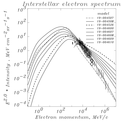
Figure 2.— Electron spectra as obtained after propagation in our models compared with direct measurements. Data: Taira et al. (1993) (vertical lines), Golden et al. (1984, 1994) (shaded areas), Ferrando et al. (1996) (small diamonds), Barwick et al. (1998) (large diamonds). Left: Thin solid line: C model, dashes: HE model, thick solid line: HEMN model, dots: SE model. Right: Electron injection spectral indices 2.0–2.4, no reacceleration.

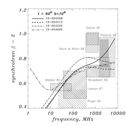
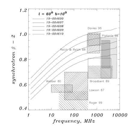
Figure 3.— Synchrotron spectral index for selected models. Measurements by different authors are shown by boxes. Data references: Webber, Simpson, & Cane (1980), Lawson et al.  (1987), Roger et al. (1999), Broadbent, Haslam, & Osborne (1989), Platania et al. (1998) (grey boxes and open box), Reich & Reich (1988), Davies, Watson, & Gutiérrez (1996). Note that the error bar given by Webber, Simpson, & Cane (1980) is probably too small due to the difficulties of low-frequency radio measurements. Left: Solid line: model C, dashes: model HE, dash-dot: model HEMN, dash-3-dots: model SE. Right: Electron injection spectral indices 2.0–2.4 (from bottom to top), no reacceleration; electron spectra as in Fig. 2 (right).

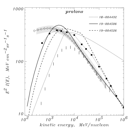
Figure 4.— Proton spectra as obtained after propagation in our models compared with IMAX data and published estimates of the interstellar spectrum. Solid line: using power-law injection spectrum (models C, HE), dashed line: with break in injection spectrum at 20 GeV (model HEMN), dotted line: hard nucleon spectrum (model HN). Vertical bars: IMAX direct measured values (Menn et al. (1997)). Evaluations of the interstellar spectrum: shaded area: based on IMAX data (Menn et al. (2000)), connected filled squares: Webber & Potgieter (1989) and Webber (1998), connected open diamonds: based on LEAP and IMP-8 (Seo et al. (1991)).

In model C (‘conventional’) the electron spectrum is adjusted to agree with the locally measured one from 10 GeV to 1 TeV and to satisfy the stringent synchrotron spectral index constraints. We show that the simple C model is inadequate for $\gamma$-rays; the remaining models represent various possibilities for improvement. Model HN (‘hard nucleon spectrum’) uses the same electron spectrum as in model C, while the nucleon spectrum is adjusted to fit the $\gamma$-ray emission above 1 GeV. This model is tested against antiproton and positron data. In model HE (‘hard electron spectrum’) the electron spectrum is adjusted to match the $\gamma$-ray emission above 1 GeV via IC emission, relaxing the requirement of fitting the locally measured electrons above 10 GeV. Model HEMN has the same electron spectrum as the HE model but has a modified nucleon spectrum to obtain an improved fit to the $\gamma$-ray data. Model HELH (‘large halo’) is like the HEMN model but with 10 kpc halo height, to illustrate the possible influence on extragalactic background estimates. Finally, in model SE (‘soft electron spectrum’) a spectral upturn in the electron spectrum below 200 MeV is invoked to reproduce the low-energy ($<$30 MeV) $\gamma$-ray emission without violating synchrotron constraints.

Even given the particle injection spectra we still have the choice of halo size and whether to include reacceleration. We have used reacceleration models here except for the more exploratory cases HN and SE. The propagation is obviously also subject to many uncertainties. The modelling of propagation can however simply be seen as a way to obtain a physically motivated set of particle spectra to be tested against $\gamma$-ray and other observations; in the end we test just the ambient electron and nucleon spectra against the data, independent of the physical nature of their origin. In this sense our investigation does not depend on the details of the propagation models but still retains the constraints imposed by antiproton and positron data.

4. Synchrotron emission

Observations of synchrotron intensity and spectral index provide essential and stringent constraints on the interstellar electron spectrum and on our magnetic field model. For this reason we discuss it first, before considering the more complex subject of $\gamma$-rays.

The synchrotron emission in 10 MHz – 10 GHz band constrains the electron spectrum in the $\sim$1–10 GeV range (see e.g. Webber, Simpson, & Cane (1980)). Out of the plane, free-free absorption is only important below 10 MHz (e.g. Strong & Wolfendale (1978)) and so can be neglected here. In particular the synchrotron spectral index ($T\propto\nu^{-\beta}$) provides information on the ambient electron spectral index $\gamma$ in this range (approximately given by $\beta=2+{\gamma-1\over 2}$ but note that we perform the correct integration over our electron spectra after propagation).

While there is considerable variation on the sky and scatter in the observations, and local variations due to loops and spurs, it is agreed that a general steepening with increasing frequency from $\beta=2.5$ to $\beta=2.8-3$ is present. Webber, Simpson, & Cane (1980) found $\beta=2.57\pm 0.03$ for 10–100 MHz. Lawson et al. (1987) give values for 38–408 MHz between $\beta=2.5$ and 2.6 using drift-scan simulations which lead to more reliable results than the original analyses (e.g. Sironi (1974): $\beta\sim 2.4$). A recent reanalysis of a DRAO 22 MHz survey (Roger et al. (1999)) finds a rather uniform 22 – 408 MHz spectral index, with most of the emission falling in the range $\beta=2.40-2.55$. Reich & Reich (1988) consider $\beta$(408–1420 MHz)$=3.1$ after taking into account thermal emission. Broadbent, Haslam, & Osborne (1989) find $\beta$(408-5000 MHz) $\sim 2.7$ in the Galactic plane, using far IR data to model the thermal emission, but remark that 3.0 may be more appropriate for a full sky average (cf. the Reich & Reich value). Davies, Watson, & Gutiérrez (1996) find an index range for 408–1420 MHz of $\beta=2.6-3.3$ for a high-latitude band, and state that 3.0 is a typical value. Recent new experiments give reliable spectral indices up to several GHz (Platania et al. (1998)); they used a catalogue of HII regions to account for thermal emission.

Fig. 3 summarizes these estimates of the Galactic nonthermal spectral index as a function of frequency. Since the electron spectrum around 1 GeV is steepened both by energy losses and energy-dependent diffusion, we can conclude from the low-frequency $\beta\sim 2.5$ that the injection spectrum must have $\gamma\leq 2.0$. In fact our models require an injection $\gamma=1.6-1.8$ to compensate the steepening and give reasonable agreement with the observed $\beta(\nu)$. Since all the models we will describe are chosen to have this injection index in the energy range producing radio synchrotron, they are all consistent with the synchrotron index constraints.

The comparison with models also depends on the $z$-distribution of the magnetic field, since this affects how the spectral index is weighted with $z$, and will give larger indices for larger extents of $B$ due the spectral steepening with $z$. Since the $z$-variation of $B$ is unknown and otherwise plays a rather secondary rôle in our model we use our predicted $\beta$ just for a representative intermediate Galactic direction ($l=60^{\circ},b=10^{\circ}$), which is taken as typical of the data with which we compare. The analysis is quite insensitive to the choice of direction.

Figure 5.— Intensity profiles of synchrotron emission at 408 MHz in latitude $(10^{\circ}\leq l\leq 60^{\circ},300^{\circ}\leq l\leq 350^{\circ})$ and longitude ($|b|\leq 5^{\circ}$) for the HEMN model. Data: Haslam et al. (1982).

             

Figure 6.— Magnetic field ($B_{tot}$) distribution at $z=0$ as used in our models (solid line) compared to parametrization by Broadbent et al. (1990) (dashes).

Figure 7.— Gamma-ray energy spectrum of the inner Galaxy ($300^{\circ}\leq l\leq 30^{\circ}$, $|b|\leq 5^{\circ}$) compared with calculations in C model (the injection spectrum chosen to fit local electron spectrum and synchrotron index). Curves show the contribution of IC, bremsstrahlung, and $\pi^{0}$-decay, and the total. Data: EGRET (Strong & Mattox (1996)), COMPTEL (Strong et al. (1999)), OSSE ($l=0,25^{\circ}$: Kinzer, Purcell, & Kurfess (1999)).

We evaluate synchrotron emission in more detail only for our model with hard electron and modified nucleon injection spectra (HEMN) since this is preferred from our $\gamma$-ray analysis in the following sections. The values of the parameters adopted in equation (1), $B_{0}$ = 6.1$\mu$G, $R_{B}$ = 10 kpc, $z_{B}$ = 2 kpc, were found to reproduce sufficiently well the synchrotron index (Fig. 3), and the absolute magnitude and profiles of the 408 MHz emission (Haslam et al. (1982)) as shown in Fig. 5. The thermal contribution in the plane at this frequency is only about $\sim$15% (Broadbent, Haslam, & Osborne (1989)). A significantly smaller field would give too low synchrotron intensites as well as a spectral index distribution which disagrees with the data, shifting the curve in the $\beta(\nu)$ plot to the left. $R_{B}$ is constrained by the longitude profile, and $z_{B}$ by the latitude profile of synchrotron emission.

For comparison, Heiles (1996) gives $B_{0}\sim$ 5$\mu$G for the volume and azimuthally averaged (uniform + random) field at the solar position based on pulsar rotation measures and synchrotron data. Vallée (1996) gives similar values. Our $B$ value follows from the attempt to include $\gamma$-ray information on the electron spectrum throughout the Galaxy and is consistent with these other estimates. The radial distribution and magnitude of the magnetic field is also consistent with that used by Broadbent et al. (1990), as shown in Fig. 7.

Our model cannot reproduce the asymmetries in latitude or fine details of the longitude distribution of synchrotron emission and this is not our goal. An exact fit to the profiles, involving spiral structure as well as explicit modelling of random and non-random field components, as in Phillipps et al. (1981), Broadbent et al. (1990), Beuermann, Kanbach, & Berkhuijsen (1985), is not attempted here.

5. Gamma-ray data

For comparison of longitude and latitude profiles we use EGRET data from Cycle 1–4 in the form of standard counts and exposure maps in 10 energy ranges (bounded by 30, 50, 70, 100, 150, 300, 500, 1000, 2000, 4000, and 10000 MeV). The systematic errors in the EGRET profiles due to calibration uncertainty and time-dependent sensitivity variations are up to 13% (Sreekumar et al. (1998)). These dominate over statistical errors in the EGRET profiles.

The contribution from point sources was removed using the following procedure. Point-like $\gamma$-ray excesses were determined in four energy regimes (30–100, 100–300, 300–1000, and $\geq$1000 MeV) using a likelihood method (Mattox et al. (1996)). A detection threshold similar to EGRET source catalogs was applied, and $\sim 280$ sources were selected by comparing with sources from the 3rd EGRET catalog (Hartman et al. (1999)). Using either the catalog spectral indices, or a –2.0 spectral index when no spectrum could be obtained, the flux of each source was subsequently integrated for the standard energy intervals. For the three brightest sources on the sky (Vela, Crab, Geminga pulsar) the flux determined in each energy interval was used directly. The simulated count distributions of the selected sources were subtracted from the summed count maps of the EGRET Cycle 1–4 data.

The $\gamma$-ray sky maps computed in our models are convolved with the EGRET point-spread function generated for an $E^{-2}$ input spectrum (the convolution is insensitive to the exact form of the spectrum). For spectral comparison at low latitudes it is better to use results based on multicomponent fitting, which accounts for the angular resolution of the instrument; here we use the results of Strong & Mattox (1996), synthesizing the skymaps of Galactic emission from their model components and parameters. Cross-checks between this approach and the direct method show excellent agreement. At high latitudes, where the convolution has negligible effect, we generate spectra directly from the EGRET Cycle 1–4 data described above.

For energies below 30 MeV only spectral data for the inner Galaxy ($330^{\circ}\leq l\leq 30^{\circ},|b|\leq 5^{\circ}$) are considered, COMPTEL: Strong et al. (1999), OSSE: Kinzer, Purcell, & Kurfess (1999). The COMPTEL low-latitude spectrum is a recent improved analysis which is about a factor 2 above that given in Strong et al. (1997) and there remains some uncertainty as discussed in Strong et al. (1999); however the difference has negligible effect on our conclusions. The COMPTEL high-latitude spectra are from Bloemen et al. (1999), Kappadath (1998), and Weidenspointner et al. (1999).

6. Model C (conventional model)

We start with a ‘conventional’ model which reproduces the local directly measured electron, proton, and Helium spectra above 10 GeV (where solar modulation is small) and which also satisfies the synchrotron constraints. The propagation parameters are taken from SM (98). This model has $z_{h}=4$ kpc, reacceleration with $v_{A}=20$ km s^-1 and a normalization chosen to best fit the local electron spectrum above 10 GeV. A break in the injection spectrum is required to fit both the synchrotron spectrum and the directly measured electron spectrum; we adopted a steepening from $-1.6$ to $-2.6$ at 10 GeV. The local electron spectrum, the synchrotron spectral index, the local proton spectrum, and the $\gamma$-ray spectrum of the inner Galaxy, are shown in Figs. 2, 3, 4, and 7, respectively.

Figure 8.— Gamma-ray energy spectrum of the inner Galaxy ($300^{\circ}\leq l\leq 30^{\circ}$, $|b|\leq 5^{\circ}$) compared with calculations for electron injection spectral indices 2.0–2.4 (from left to right, top to bottom) as shown in Fig. 3. Curves show the contribution of IC, bremsstrahlung, and $\pi^{0}$-decay, and the total. Data: as in Fig. 7.

             

Figure 9.— Interstellar antiproton flux for models (MSR (98)) compared with local measurements. Solid line: C, dotted line: HN, dashed line: HEMN. Data (direct measurements): triangles: MASS91 experiment (Basini et al. (1999)), other points: see references in MSR (98).

Figure 10.— Interstellar positron spectra for models compared with data. Solid line: model C, dotted line: HN, dashed line: HEMN. Data (direct measurements): HEAT experiment (Barwick et al. (1998)).

Model C is based entirely on non-$\gamma$-ray data but still approximates the $\gamma$-ray data within a factor 3 over three decades of energy (10 MeV to 10 GeV). It also satisfies the limits imposed by antiprotons and positrons (MSR (98), Moskalenko & Strong 1998b, hereafter MS98b ), though our new calculation shows some deficit of positrons below $\approx 10$ GeV (Figs. 10 and 10, see also discussion in Section 7.1). It still remains a useful first approximation to serve as the basis for the developments which follow.

The fit to the inner Galaxy $\gamma$-ray spectra is satisfactory from 30 to 500 MeV but a large excess in the EGRET spectrum relative to the predictions above 1 GeV is evident, as first pointed out by Hunter et al. (1997). Simple rescaling of either electron or nucleon spectra does not allow the agreement to be signficantly improved. Harder nucleon or electron spectra are therefore investigated below.

The model also fails to account for the $\gamma$-ray intensities below 30 MeV as observed by COMPTEL and OSSE; attempting to account for this with a steeper electron spectrum immediately violates the synchrotron constraints, unless the steepening occurs at electron energies below a few hundred MeV, as discussed in Section 7.3 (model SE). To prove this important point, we consider a series of electron injection indices 2.0–2.4 in a model without reacceleration and diffusion coefficient index $\delta=1/3$; this conveniently spans the range of reasonably simple electron spectra. Fig. 2 (right) shows these electron spectra, and Fig. 3 (right) the corresponding synchrotron indices. The corresponding gamma-ray spectra are shown in Fig. 8. It is clear that an index 2.2–2.3 is required to fit the $\gamma$-rays, while this produces a synchrotron index about 0.8 which is substantially above that allowed by the data. Although this is for a particular propagation model, note that any combination of injection and propagation which fits the $\gamma$-rays will have the same problem, except for extreme models (e.g. our SE model).

We emphasize that it is the synchrotron constraint on the electron index which forces us to this conclusion; in the absence of this we would be free to adopt a uniformly steep electron injection spectrum to obtain a fit to the low-energy $\gamma$-rays. This is the essential difference between present and earlier work (e.g. Strong (1996), SM (97)) where the consequences of the synchrotron constraints were not fully appreciated.

Figure 11.— Gamma-ray data as in Fig. 7 compared with HN model (hard nucleon spectrum chosen to fit EGRET data above 1 GeV).

7. Beyond the conventional models

7.1. HN model (hard nucleon spectrum)

One possibility to reproduce the $\gamma$-ray excess above 1 GeV is to invoke interstellar proton and Helium spectra which are harder than those directly observed in the heliosphere (Gralewicz et al. (1997), Mori (1997)). Spatial variations in the nucleon spectrum are quite possible over the Galaxy so that such an option is worth serious consideration. This model has been studied in detail in MSR (98) in relation to antiprotrons, so that here we just summarize the results and also extend the calculation to secondary positrons. The $\gamma$-ray spectrum of the inner Galaxy for a model with a hard nucleon injection spectrum chosen to match the $\gamma$-rays (no reacceleration, proton and He injection index = 1.7) is shown in Fig. 11. The corresponding propagated interstellar proton spectrum is shown in Fig. 4.

As pointed out in MSR (98), the same nucleons which contribute to the GeV $\gamma$-ray emission through the decay of $\pi^{0}$-mesons produce also secondary antiprotons and positrons (on the same interstellar matter). The harder nucleon spectrum hypothesis, therefore, can be tested with measurements of CR $\bar{p}$’s and $e^{+}$’s (MSR (98), MS98b ). Above $T_{p}\sim$ few 10 GeV (for a power-law proton spectrum) the mean kinetic energy of parent protons is about 10 times larger than that of produced secondary $\bar{p}$’s, and roughly the same holds for $\gamma$-rays, so 10 GeV $\bar{p}$’s and $\gamma$’s both are produced by $\sim 100$ GeV nucleons. This relation is also valid for secondary positrons. Such tests are therefore well tuned, and sample the Galactic-scale properties of CR $p$ and He rather than just the local region, independent of fluctuations due to local primary CR sources.

The conclusion of MSR (98), based on the $\bar{p}/p$ ratio as measured by Hof et al. (1996), was that antiprotons provide a sensitive test of the interstellar nucleon spectra, and that a hard nucleon spectrum overproduces $\bar{p}$’s at GeV energies. In Fig. 10 the predicted flux of antiprotons is compared with new absolute $\bar{p}$ fluxes above 3 GeV from the MASS91 experiment (Basini et al. (1999)). While the agreement is good for the normal nucleon spectrum, the hard nucleon spectrum produces too many antiprotons by a factor of $\sim 5$, well outside the error bars of the three data points. We conclude that such a hard nucleon spectrum is inconsistent with the antiproton data.

Fig. 10 shows the interstellar positron spectrum for the conventional and hard nucleon spectra, where we used the formalism given in MS98a . The flux for the conventional case agrees with recent data (Barwick et al. (1998)) at high energies, where solar modulation is not so important. For the hard nucleon spectrum the flux is higher than observed by factor $\sim$4; this provides more evidence against a hard nucleon spectrum. However this test is less direct than $\bar{p}$ due to the difference in particle type, the large effect of energy losses, and the effect of solar modulation at lower positron energies.

Taken together, the antiproton and positron data provide rather substantial evidence against the idea of explaining the $>$1 GeV $\gamma$-ray excess with a hard nucleon spectrum.

             

Figure 12.— Gamma-ray data as in Fig. 7 compared with HE model (electron injection index $-1.7$).

Figure 13.— Gamma-ray data as in Fig. 7 compared with HEMN model (electron injection index $-1.8$, and modified nucleon spectrum).

Note that in these tests we assume that only the protons have a local spectrum which is different from that on Galactic scales. We assume that the propagation parameters can still be derived from B/C, so that implicitly the heavier nuclei C, O are not affected. We could alternatively adopt a picture in which the C, O etc. also have a local spectrum different from Galactic scales, but then fitting the B/C ratio would imply $\delta>0.6$ for the index in the diffusion coefficient (nonreacceleration case) which is certainly problematic for high-energy anisotropy (see SM (98) and references therein) and larger than predicted by standard diffusion theory. Therefore we consider the only case worth testing at this stage is the one where only the protons are affected. In any case, pursuit of more complex options is beyond the scope of this paper.

7.2. A harder interstellar electron spectrum (HE & HEMN models)

An obvious way to improve the fit to the EGRET data above 1 GeV is to adopt a harder interstellar electron injection spectrum. Such models will not match the directly-observed electron spectrum above 10 GeV, but this is not critical since the large energy losses in this region mean that large spatial fluctuations are expected (Pohl & Esposito (1998)). Hence we relax the constraint of consistency with the locally measured electron spectrum.

For the HE model we adjust the electron injection index and the absolute electron flux to optimize the fit to the inner-Galaxy $\gamma$-ray spectrum; also the absolute nucleon intensity ($\pi^{0}$-component) was reduced slightly (factor 0.8) within the limits allowed by the proton and Helium data. The inner-Galaxy $\gamma$-ray spectrum is shown in Fig. 13. This model with its harder electron injection index ($-1.7$) satisfies the synchrotron constraints and also leads to a better fit to the $\gamma$-rays above 1 GeV, but produces too few $\gamma$-rays at energies below 30 MeV by a factor 2–4. In this case the additional low energy $\gamma$-rays must be attributed to another component as discussed in Section 7.3 in the context of SE model.

Pohl & Esposito (1998) use an electron injection index 2.0 with a Gaussian distribution of 0.2 for their $\gamma$-ray model. This has the effect of an upwards curvature which is equivalent to a harder spectrum similar to ours. Quantitatively, from their Fig. 4, the difference in effective index for their spiral arm model going from a single index to the index with dispersion gives in fact a difference 0.2 at high energies. So the dispersed index is equivalent to a single index, 2.0–0.2 = 1.8, which is similar to our 1.7 (HE model).

Since the fit of HE model to the EGRET detailed spectral shape is still not very good above 1 GeV we can ask whether it can be improved by allowing more freedom in the nucleon spectrum also (model HEMN). Some freedom is allowed since solar modulation affects direct measurements of nucleons below 20 GeV, and the locally measured nucleon spectrum may not necessarily be representative of the average on Galactic scales either in spectrum or intensity due to details of Galactic structure (e.g. spiral arms). Because of the hard electron spectrum the required modification to the nucleon spectrum is much less drastic than in model HN. By introducing an ad hoc flattening of the nucleon spectrum below 20 GeV, a small steepening above 20 GeV, and a suitable normalization, an improved match to the inner Galaxy EGRET spectrum is indeed possible (Fig. 13). The spectral parameters are given in Table 1. For the modified nucleon spectrum (Fig. 4) we must invoke departures from cylindrical symmetry so that the local value still agrees with direct measurements at the solar position. However this modification of the nucleon spectrum must be checked against the stringent constraints on the interstellar spectrum provided by antiprotons and positrons (as in model HN). The predictions of this model are shown in Figs. 10 and 10. As expected the predictions are larger than the conventional model but still within the antiproton and positron limits.

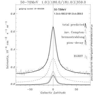
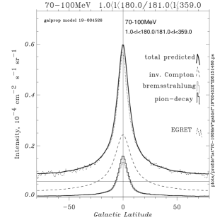
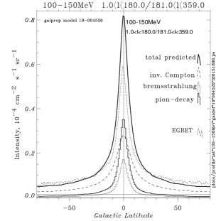
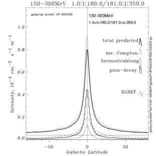
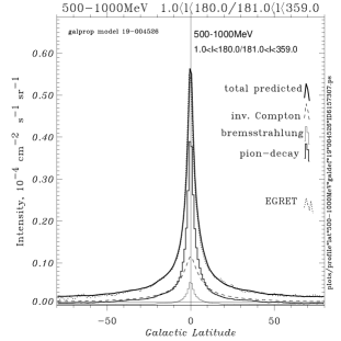
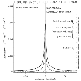
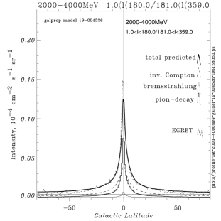
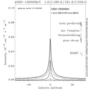
Figure 14.— Latitude distribution of $\gamma$-rays ($0^{\circ}\leq l\leq 360^{\circ}$) for model HEMN (thick solid line). Separate components show the contribution of IC (dashes), bremsstrahlung (thin histogram), $\pi^{0}$-decay (thick histogram), horizonal line: isotropic background. EGRET data: dotted line.

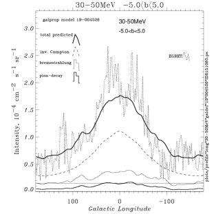
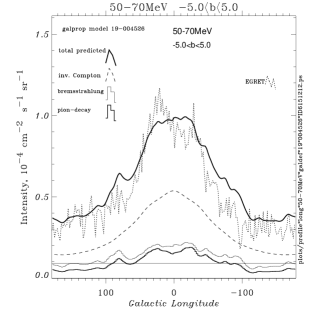
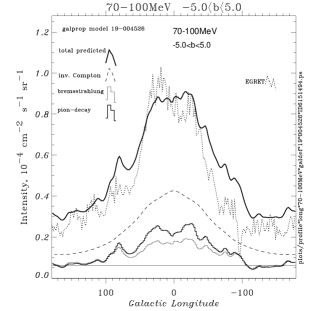
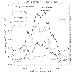
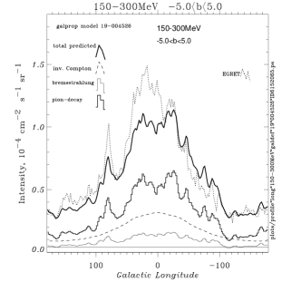
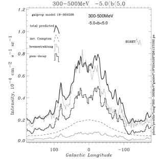
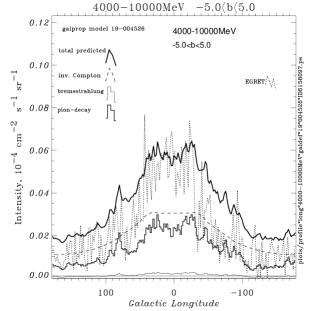
Figure 15.— Longitude distribution of $\gamma$-rays ($|b|\leq 5^{\circ}$) for model HEMN. Coding of lines for components is the same as in Fig. 14. EGRET data: dotted line.

             

Figure 16.— High latitude distribution (enlarged) of 70–100 MeV $\gamma$-rays from the EGRET compared to model HEMN. Lines are coded as in Fig. 14.

Figure 17.— Gamma-ray data as in Fig. 7 compared with SE model (electron injection spectrum with upturn below 200 MeV).

So far this is the most promising model (at least for $\gamma$-rays $>$30 MeV) and hence we consider it further by testing the angular distribution of the emission. The synchrotron predictions for this model and comparison with data were presented in Section 4. Figs. 14 and 15 show the HEMN model latitude and longitude $\gamma$-ray distributions convolved with the EGRET point-spread function, compared to EGRET Phase 1–4 data. The separate components are also shown. Since the isotropic component is here regarded as a free parameter it was adjusted in each energy range to give agreement with the high-latitude intensities in the latitude plots, and the same value was used in the longitude plots.

In latitude the agreement is always quite good, in longitude the maximum deviation is about 25% in the 100–150 MeV, 150–300 MeV, and 4–10 MeV ranges, typically the agreement is better than 10%. We believe, this is satisfactory for a model which has not been optimized for the spatial fit in each energy range, but anyway these figures allow the reader to judge for himself. In any case, it should be remembered that unresolved point-source components and irregularities in the cosmic-ray source distribution are expected to lead to deviations from our cylindrically symmetrical model at some level.

In this model the contributions to the spectrum of the inner Galaxy from IC and $\pi^{0}$-decay are about equal at 100 MeV and 6 GeV, $\pi^{0}$-decay dominates between these energies, and bremsstrahlung produces $\lesssim$10% of the total. The comparison shows that a model with large IC component can indeed reproduce the data. A profile for 70–100 MeV enlarged to illustrate the high-latitude variation (Fig. 17) shows that this model also accounts very well for the observed emission; we regard this as support for the large IC halo concept.

Turning to high energies, consider the latitude and longitude profiles for 4000–10000 MeV; the agreement shows that the adoption of a hard electron injection spectrum is a viable explanation for the $>$1 GeV excess. The latitude distribution here is not as wide as at low energies owing to the rapid energy losses of the electrons; both HN and HEMN models reproduce the observed spectrum, and latitude and longitude profiles almost equally well (MS98b ), and hence it is difficult to discriminate between them on the basis of $\gamma$-rays alone. Independent tests however argue against HN as described in Section 7.1.

It is interesting to note that in fitting EGRET data Strong & Mattox (1996) found that the IC component had a harder spectrum than expected (see their Fig. 4), which was quite puzzling at that time. Also the study of Chen, Dwyer, & Kaaret (1996) at high latitudes found a hard IC component. These results can now be understood in the context of the HE or HEMN model; a renewed application of the fitting approach with the new models would be worthwhile and is intended for the future. All these results can be taken as adding support to the ‘hard electron spectrum’ interpretation of the $\gamma$-ray results, and for the idea that the average interstellar electron spectrum is harder than that measured in the heliosphere.

If this model is indeed correct it then implies that bremsstrahlung plays a rather minor rôle at all energies, contrary to previous ideas, with IC and $\pi^{0}$-decay accounting for $\sim$90% of the diffuse emission.

Although we have introduced rather arbitrary modifications to both electron and nucleon spectra to better fit the $\gamma$-ray data, we note two recent indications that add support to our approach from independent studies. Baring et al. (1999) recently presented models for shock acceleration in SNR which produce very flat electron spectra quite similar to what we require in the present case. Further study of the possible link between these spectra is in progress. A completely independent line of evidence for a low-energy flattening of the proton spectrum has recently been presented by Lemoine, Vangioni-Flam, & Cassé (1998), based on cosmic-ray produced light element abundances. If the proton and He spectra do differ from that locally measured, this could of course also apply other primaries, but an investigation of this is beyond the scope of the present work, which focusses on $\gamma$-rays.

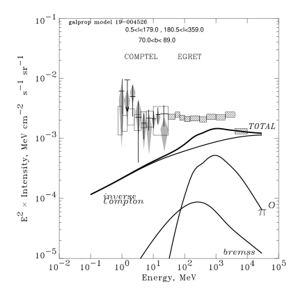
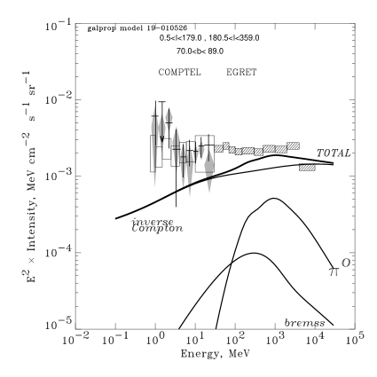
Figure 18.— Energy spectrum of $\gamma$-rays from high Galactic latitudes ($|b|\geq 70^{\circ}$, all longitudes) for HEMN model (left) and HELH model (right). Shaded areas: EGRET total intensity from Cycle 1–4 data. COMPTEL data: high-latitude total intensity (open boxes: Bloemen et al. (1999), diamonds: Kappadath (1998), crosses: Weidenspointner et al. (1999)).

7.3. A steeper spectrum of electrons at low energies (SE model) or a population of MeV point sources in the Galactic plane ?

In order to reproduce the low-energy ($<$ 30 MeV) $\gamma$-ray emission via diffuse processes it is necessary to invoke steepening of the electron spectrum below about 200 MeV to compensate the increasing ionization losses. A steep slope continuing to higher energies would violate the synchrotron constraints on the spectral index, as discussed in Section 5. For illustration we show a non-reacceleration model with an injection index –3.2 below 200 MeV, and –1.8 above (SE model). This fits both the COMPTEL and EGRET data (Fig. 17) while remaining consistent with the synchrotron constraints (Fig. 3). The synchrotron index increase occurs at frequencies $<10$ MHz, below the range where useful limits can be set (see Strong & Wolfendale (1978)). Although the behaviour of the electron diffusion coefficient at energies below 100 MeV is quite uncertain (Bieber et al. (1994)) the propagated spectrum is here dominated by energy losses, which severely limit the electron range, so that this is not critical for our model.

In this model 70% of the emission is bremsstrahlung and 30% IC at 1 MeV. This is the only model in the present work which can reproduce the entire $\gamma$-ray spectrum. A possible mechanism for acceleration of low-energy electrons has been proposed by Schlickeiser (1997). However the adoption of such a steep low-energy electron spectrum has problems associated with the very large power input to the interstellar medium (Skibo et al. (1997)), and is ad hoc with no independent supporting evidence. Moreover the OSSE-GINGA $\gamma$-ray spectrum is steeper than $E^{-2}$ below 500 keV (Kinzer, Purcell, & Kurfess (1999)) which would require an even steeper electron injection spectrum than adopted here. It is more natural to consider that the COMPTEL excess is just a continuation of the same component producing the OSSE-GINGA spectrum. Most probably therefore the excess emission at low energies is produced by a population of sources such as supernova remnants, as has been proposed for the diffuse hard X-ray emission from the plane observed by RXTE (Valinia & Marshall (1998)), or X-ray transients in their low state as suggested for the OSSE diffuse hard X-rays (Lebrun et al. (1999)). The contribution from point sources is then about 70% at 1 MeV, the rest being IC. Above 10 MeV the diffuse emission dominates. Yamasaki et al. (1997) estimate a 20% contribution from point sources to the hard X-ray plane emission, the rest being attributed to young electrons in SNR, but these are still localized $\gamma$-ray sources rather than truly diffuse emission.

A model with a constant electron injection index –2.4 can also fit the low-energy $\gamma$-rays, but conflicts with the synchrotron index and fails to reproduce the high-energy $\gamma$-rays. While this has been a popular option in the past (e.g., Strong (1996)), it cannot any longer be considered plausible.

We note that another possible origin for the low-energy $\gamma$-rays, synchrotron radiation from $\sim$100 TeV electrons, has been suggested by Porter & Protheroe (1997).

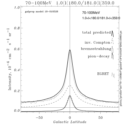
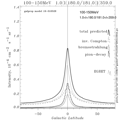
Figure 19.— High latitude distribution of $\gamma$-rays for HELH model, 70–100 MeV (left), and 100–150 MeV (right), compared to EGRET data. Lines are coded as in Fig. 14.

Figure 20.— Gamma-ray luminosity spectrum of diffuse emission from the whole Galaxy using HEMN model (left), and HELH model (right). Total is shown as solid line. Separate components: IC (dashes), bremsstrahlung (dots), and $\pi^{0}$-decay (dash-dot).

8. High latitude $\gamma$-rays and the size of the electron halo

Gamma rays provide a tracer of the electron halo via IC emission. In considering the HEMN model we showed that the high-latitude variation of EGRET $\gamma$-rays is in good agreement with our large IC halo concept (Fig. 17, Section 7.2). Indication for a large $\gamma$-ray halo was also found by Dixon et al. (1998) from analysis of EGRET data. Although we have used $z_{h}=4$ kpc as the standard value in the present work we now test larger values to derive limits. Studies of ¹⁰Be (SM (98)) gave the range $z_{h}=4-12$ kpc for nucleons. Webber & Soutoul (1998) find $z_{h}=2-4$ kpc from ¹⁰Be and ²⁶Al data. Ptuskin & Soutoul (1998) find $z_{h}=4.9^{+4}_{-2}$ kpc. The high latitude $\gamma$-ray intensity increases with halo size due to IC emission (though much less than linearly due to electron energy losses), so that at least an upper limit on the halo size can be obtained. Fig. 18 shows the $\gamma$-ray spectrum towards the Galactic poles for $z_{h}=4$ kpc (HEMN model), and 10 kpc (HELH model). $z_{h}=10$ kpc is possible although the latitude profile for the 100–150 MeV range is then very broad and at the limit of consistency with EGRET data (Fig. 19). Further the isotropic component would have to approach zero above 300 MeV, so that this halo size can be considered an upper limit.

If the halo size is 4–10 kpc as we argue, the contribution of Galactic emission to the total at high latitudes is larger than previously considered likely and has consequences for the derivation of the diffuse extragalactic emission (e.g., Sreekumar et al. (1998)). An evaluation of the impact of our models on estimates of the extragalactic spectrum is beyond the scope of the present work.

9. Luminosity spectrum of our Galaxy

So far some 90 extragalactic sources have been observed with the EGRET telescope and several with COMPTEL (e.g., Hartman et al. (1997), 1999). Most of these sources are blazars. Such data usually serve as a basis for estimates of the extragalactic $\gamma$-ray background radiation. However, the number of normal galaxies far exceeds that of active galaxies, it is therefore interesting to calculate the total diffuse continuum emission of our Galaxy as an example. Using cosmological evolution scenarios, this can then be used as the basis for estimates of the contribution from normal galaxies to the extragalactic background.

The luminosity spectrum of the diffuse emission from the Galaxy is shown in Fig. 20, based on models HEMN (4 kpc halo) and HELH (10 kpc halo). The total $\gamma$-ray diffuse luminosity of the Galaxy above 1 MeV is $L_{G}=7.1\times 10^{39}$ erg s^-1 for the HEMN model and $9.2\times 10^{39}$ erg s^-1 for the HELH model. Above 100 MeV the values are $5.4\times 10^{39}$ erg s^-1 and $6.3\times 10^{39}$ erg s^-1, respectively. These values are higher than previous estimates (e.g. Bloemen, Blitz, & Hermsen (1984): $[1.6-3.2]\times 10^{39}$ erg s^-1 above 100 MeV) due to our large halo and the fact that our model incorporates the EGRET GeV excess.

10. Conclusions

We have carried out a new study of the diffuse Galactic $\gamma$-ray continuum radiation using a cosmic-ray propagation model including nucleons, electrons, antiprotons, positrons, and synchrotron emission.

We have shown that ‘conventional’ models based on locally measured cosmic-ray spectra are consistent with $\gamma$-ray measurements in the 30–500 MeV range, but outside this range excesses are apparent. A harder nucleon spectrum alone is considered but fitting to $\gamma$-rays causes it to violate limits from positrons and antiprotons. A harder interstellar electron spectrum allows the $\gamma$-ray spectrum to be fitted also above 1 GeV, and this can be further improved when combined with a modified nucleon spectrum which still respects the limits imposed by antiprotons and positrons. This is our preferred model, and it matches the EGRET $\gamma$-ray longitude and latitude profiles reasonably in each energy band.

Such a model produces only 25–50% of the 1–30 MeV emission by diffuse processes. The constraints provided by the synchrotron spectral index do not allow all of the $<$30 MeV $\gamma$-ray emission to be explained in terms of a steep electron spectrum unless this takes the form of a sharp upturn below 200 MeV. Therefore we prefer a source population as the origin of the excess low-energy $\gamma$-rays, which can then be seen as an extention of the hard X-ray continuum measured by OSSE, GINGA and RXTE. This is a quite natural scenario since it is very likely that the hard X-rays are indeed from unresolved sources, and the switchover from source-dominated to diffuse-dominated has to occur at some point; we propose here that it occurs at MeV energies.

The large electron/IC halo suggested here reproduces well the high-latitude variation of $\gamma$-ray emission, which can be taken as support for the halo size for nucleons deduced from independent studies of cosmic-ray composition. Halo sizes in the range $z_{h}=4-10$ kpc are favoured by both analyses.

Our models suggest that bremsstrahlung plays a rather minor rôle, producing not more than $\sim$10% of the Galactic emission at any energy.

Appendix A A.  Spectrum of Electron Bremsstrahlung in the ISM

In order to calculate the electron bremsstrahlung spectrum in the interstellar medium, which includes neutral gas (hydrogen and Helium), hydrogen-like and Helium-like ions as well as the fully ionized medium, we use the works of Koch & Motz (1959), Gould (1969), and Blumenthal & Gould (1970). Our approach is similar to that used by Sacher & Schönfelder (1984), but differs in some details. Throughout this Section the units $\hbar=c=m_{e}=1$ are used.

The important parameter is the so-called screening factor defined as

$$\delta=\frac{k}{2\gamma_{0}\gamma},$$ (A1)

where $k$ is the energy and momentum of the emitted photon, $\gamma_{0}$ and $\gamma$ are the initial and final Lorentz factor of the electron in the collision. If $\delta\to 0$, the distance of the high energy electron from the target atom is large compared to the atomic radius. In this case screening of the nucleus by the bound electrons is important. Otherwise, for the low-energy electron only the contribution of the nucleus is important, while at high energies the atomic electrons can be treated as unbound and can be taken into account as free charges.

The cross section for electron-electron bremsstrahlung with one electron initially at rest approaches, at high energies ($\gamma_{0},\gamma,k\gg 1$), the electron-proton bremsstrahlung cross section with the proton initially at rest (Gould (1969)). Therefore the contribution of atomic electrons at high energies can be accounted for by a factor of $(Z^{2}+N)$ in place of $Z^{2}$ in the formulas for the unshielded charge, where $Z$ is the atomic number, and $N$ is the number of the atomic electrons. In the present paper we treat free electrons in the ionized medium in the same way as protons, which is an approximation, but it provides reasonable accuracy for the range 3–200 MeV where the bremsstrahlung contribution into the diffuse emission is most important. In any case the contribution from the ionized medium is of minor importance in comparison with that of the neutral gas.

A.1. A.1.  Low energies ($0.01\leq E_{\rm kin}\leq 0.07$ MeV)

This is the case of nonrelativistic nonscreened bremsstrahlung, $\Delta\equiv\delta/(2\alpha_{f}Z^{1/3})\gg 1$. In the Born approximation ($2\pi Z\alpha_{f}/\beta_{0}$, $2\pi Z\alpha_{f}/\beta\ll 1$) the production cross section is given by eq. 3BN(a) from Koch & Motz (1959)

$$\frac{d\sigma}{dk}=f_{E}\frac{16}{3}\frac{Z^{2}r_{e}^{2}\alpha_{f}}{kp_{0}^{2}}\ln\left(\frac{p_{0}+p}{p_{0}-p}\right),$$ (A2)

where $\alpha_{f}$ is the fine structure constant, $p_{0}$ and $p$ are initial and final momentum of the electron in the collision, $\beta_{0}$ and $\beta$ are initial and final velocity of the electron, and $f_{E}$ is the Elwert factor,

$$f_{E}=\frac{\beta_{0}[1-\exp(-2\pi Z\alpha_{f}/\beta_{0})]}{\beta[1-\exp(-2\pi Z\alpha_{f}/\beta)]},$$ (A3)

which is a correction for the cross section eq. (A2) at nonrelativistic energies.

A.2. A.2.  Intermediate energies ($0.07\leq E_{\rm kin}\leq 2$ MeV)

For the case of nonscreened bremsstrahlung ($\Delta\gg 1$) the Born approximation cross section is given by (Koch & Motz (1959), eq. 3BN):

$$\frac{d\sigma}{dk} = \xi f_{E}Z^{2}r_{e}^{2}\alpha_{f}\frac{p}{kp_{0}}\left\{\frac{4}{3}-2\gamma_{0}\gamma\frac{p^{2}+p_{0}^{2}}{p_{0}^{2}p^{2}}+\frac{\epsilon_{0}\gamma}{p_{0}^{3}}+\frac{\epsilon\gamma_{0}}{p^{3}}-\frac{\epsilon\epsilon_{0}}{pp_{0}}\right.$$ (A4)

$$\left.+L\left[\frac{8}{3}\frac{\gamma_{0}\gamma}{p_{0}p}+k^{2}\frac{\gamma_{0}^{2}\gamma^{2}+p_{0}^{2}p^{2}}{p_{0}^{3}p^{3}}+\frac{k}{2p_{0}p}\left(\epsilon_{0}\frac{\gamma_{0}\gamma+p_{0}^{2}}{p_{0}^{3}}-\epsilon\frac{\gamma_{0}\gamma+p^{2}}{p^{3}}+2k\frac{\gamma_{0}\gamma}{p^{2}p_{0}^{2}}\right)\right]\right\},$$

where

$$\epsilon_{0}=\ln\left(\frac{\gamma_{0}+p_{0}}{\gamma_{0}-p_{0}}\right),$$

$$\epsilon=\ln\left(\frac{\gamma+p}{\gamma-p}\right),$$

$$L=2\ln\left[\frac{\gamma_{0}\gamma+p_{0}p-1}{k}\right].$$

The factor $\xi$ is given by

$$\xi=\left[1+\frac{N}{Z^{2}}\left(1-e^{(b-E_{\rm kin})/9b}\right)\right]\left(1-0.3\,e^{-k/c}\right)$$ (A6)

where $b=0.07$ MeV, $c=0.33$ MeV, and the expression in square brackets is a correction for the contribution of $N$ atomic electrons, which is negligible at $E_{\rm kin}\sim 0.1$ MeV, but becomes as large as that of the protons at $E_{\rm kin}\sim 2$ MeV (see also general comments at the beginning of Appendix A). The second factor, in round brackets, is a correction to obtain a smooth connection between the approximations in the transition region near 0.1 MeV and is essential only for small $k$.

A.3. A.3.  High energies ($E_{\rm kin}\geq 2$ MeV)

For the case of arbitrary screening we use eq. 3BS(b) from Koch & Motz (1959):

$$\frac{d\sigma}{dk}=r_{e}^{2}\alpha_{f}\frac{1}{k}\left[\left(1+\frac{\gamma^{2}}{\gamma_{0}^{2}}\right)\phi_{1}-\frac{2}{3}\frac{\gamma}{\gamma_{0}}\phi_{2}\right].$$ (A7)

If the scattering system is an unshielded charge, the functions are $\phi_{1}=\phi_{2}=Z^{2}\phi_{u}$, where

$$\phi_{u}=4\left[\ln\left(\frac{2\gamma_{0}\gamma}{k}\right)-\frac{1}{2}\right].$$ (A8)

For the case where the scattering system is a nucleus with bound electrons, the expressions for $\phi_{1}$ and $\phi_{2}$ are more complicated and depend on the atomic form factor.

Corresponding expressions for one- and two-electron atoms ($N=1,2$) have been given by Gould (1969). Rearranging these one can obtain

$$\phi_{1}(N) = (Z-N)^{2}\phi_{u}+8Z\left\{1-\frac{N-1}{Z}+\int_{\delta}^{1}dq\,\frac{R_{N}(q)}{q^{3}}(q-\delta)^{2}\right\},$$ (A9)

$$\phi_{2}(N) = (Z-N)^{2}\phi_{u}+8Z\left\{\frac{5}{6}\left(1-\frac{N-1}{Z}\right)+\int_{\delta}^{1}dq\,\frac{R_{N}(q)}{q^{4}}\left[q^{3}-6\delta^{2}q\ln(q/\delta)+3\delta^{2}q-4\delta^{3}\right]\right\},$$

where

$$\begin{array}[]{ll}\displaystyle{R_{1}(q)=1-F_{1}(q)},&\displaystyle{F_{1}(q)=\{1+q^{2}/[2\alpha_{f}Z]^{2}\}^{-2}};\\ \displaystyle{R_{2}(q)=2[1-F_{2}(q)]-[1-F_{2}^{2}(q)]/Z},&\displaystyle{F_{2}(q)=\{1+q^{2}/[2\alpha_{f}(Z-5/16)]^{2}\}^{-2}}.\end{array}$$ (A10)

Equations (A9), (A10) are valid for any $Z$, including H^- ions. The formulas have been obtained under the assumption that the two-electron wave function of He-like atoms can be approximated by the product of one-electron functions in the form of Hylleraas or Hartree. For large $\Delta$ the expressions for $\phi_{1}$ and $\phi_{2}$ approach the unshielded value

$$\phi_{1}=\phi_{2}\to(Z^{2}+N)\phi_{u}.$$

For the case of neutral He atoms Gould (1969) gives also numerical values of $\phi_{1}$ and $\phi_{2}$ tabulated for the variable $\{\delta/(2\alpha_{f})\}=0...10$. The latter have been calculated for a Hartree-Fock wave function, which are considered to be more accurate than the Hylleraas function. At low energies ($\Delta\gtrsim 2$) both functions provide the identical results.

At high energies where $k,\gamma_{0},\gamma\gg 1$, $\Delta\gtrsim 4$, eq. (A4) with $\xi=1+N/Z^{2}$ and $f_{E}=1$ can be applied, where electrons are treated as unbound in the same way as protons.

A.4. A.4.  Fano-Sauter Limit

The formulas described above do not permit the evaluation of the cross section at the high-frequency limit $k\to\gamma_{0}-1$. The cross section obtained in the Born-approximation becomes zero in this limit, while the value is non-zero. The corresponding expression has been obtained by Fano in the Sauter approximation (Koch & Motz (1959)):

$$\left(\frac{d\sigma}{dk}\right)_{FS}=4\pi Z^{3}\alpha_{f}^{2}r_{e}^{2}\frac{\gamma_{0}\beta_{0}}{k(\gamma_{0}-1)^{2}}\left\{\frac{3}{4}+\frac{\gamma_{0}(\gamma_{0}-2)}{\gamma_{0}+1}\left[1-\frac{1}{2\beta_{0}\gamma_{0}^{2}}\ln\left(\frac{1+\beta_{0}}{1-\beta_{0}}\right)\right]\right\}.$$ (A11)

A.5. A.5.  Heavier atoms

For the electron bremsstrahlung on neutral atoms heavier than He we use the Schiff formula (Koch & Motz (1959), eq. 3BN(e)):

$$\frac{d\sigma}{dk} = 2Z^{2}r_{e}^{2}\alpha_{f}\frac{1}{k}\left\{\left(1+\frac{\gamma^{2}}{\gamma_{0}^{2}}-\frac{2}{3}\frac{\gamma}{\gamma_{0}}\right)\left(\ln M(0)+1-\frac{2}{b}\arctan b\right)\right.$$

$$\left.+\frac{\gamma}{\gamma_{0}}\left[\frac{2}{b^{2}}\ln(1+b^{2})+\frac{4(2-b^{2})}{3b^{3}}\arctan b-\frac{8}{3b^{2}}+\frac{2}{9}\right]\right\},$$

where

$$b=\frac{Z^{1/3}}{111\delta};\qquad M(0)=\frac{1}{\delta^{2}(1+b^{2})}.$$

Appendix B B.  Synchrotron radiation

For synchrotron emission we use the standard formula (see e.g. Ginzburg (1979)). After averaging over the pitch angle for an isotropic electron distribution, this gives the emissivity $\epsilon(\nu,\gamma)$ of a single electron integrated over all directions relative to the field in the form (Ghisellini, Guilbert, & Svensson (1988))

$$\epsilon(\nu,\gamma)=4\sqrt{3}\,\pi r_{e}m_{e}c\,\nu_{B}\,x^{2}\left\{K_{4/3}(x)K_{1/3}(x)-{3\over 5}x\,[K_{4/3}^{2}(x)-K_{1/3}^{2}(x)]\right\}$$ (B1)

in units of (ergs s^-1 Hz^-1), where $\nu$ is the radiation frequency, $\gamma$ is the electron Lorentz factor, $\nu_{B}=eB/(2\pi m_{e}c)$, $B$ is the total magnetic field strength, $x\equiv\nu/(3\gamma^{2}\nu_{B})$, and $K_{z}$ is the modified Bessel function of order $z$.

References

- Baring et al. (1999) Baring, M. G., et al. 1999, ApJ, 513, 311
- Barwick et al. (1998) Barwick, S. W., et al. 1998, ApJ, 498, 779
- Basini et al. (1999) Basini, G., et al. 1999, in Proc. 26th Int. Cosmic Ray Conference (Salt Lake City), 3, 77
- Berezinskii et al. (1990) Berezinskii, V. S., et al. 1990, Astrophysics of Cosmic Rays (Amsterdam: North Holland)
- Beuermann, Kanbach, & Berkhuijsen (1985) Beuermann, K., Kanbach, G., & Berkhuijsen, E. M. 1985, A&A, 153, 17
- Bieber et al. (1994) Bieber, J. W., et al. 1994, ApJ, 420, 294
- Bloemen (1985) Bloemen, H. 1985, A&A, 145, 391
- Bloemen, Blitz, & Hermsen (1984) Bloemen, J. B. G. M., Blitz, L., & Hermsen, W. 1984, ApJ, 279, 136
- Bloemen et al. (1999) Bloemen, H., et al. 1999, Astrophys. Lett. & Comm., 39, 205
- Blumenthal & Gould (1970) Blumenthal, G. R., & Gould, R. J. 1970, Rev. Mod. Phys., 42, 237
- Broadbent, Haslam, & Osborne (1989) Broadbent, A., Haslam, C. G. T., & Osborne, J. L. 1989, MNRAS, 237, 381
- Broadbent et al. (1990) Broadbent, A., et al. 1990, in Proc. 21st Int. Cosmic Ray Conference (Adelaide), 3, 229
- Cardelli, Clayton, & Mathis (1989) Cardelli, J. A., Clayton, G. C., & Mathis, J. S. 1989, ApJ, 345, 245
- Chen, Dwyer, & Kaaret (1996) Chen, A., Dwyer, J., & Kaaret, P. 1996, ApJ, 463, 169
- Chi & Wolfendale (1991) Chi, X., & Wolfendale, A. W. 1991, J. Phys. G: Nucl. Part. Phys., 17, 987
- Cox & Mezger (1989) Cox, P., & Mezger, P. G. 1989, A&A Rev., 1, 49
- Davies, Watson, & Gutiérrez (1996) Davies, R. D., Watson, R. A., & Gutiérrez, C. M. 1996, MNRAS, 278, 925
- Dixon et al. (1998) Dixon, D. D., et al. 1998, New Astron., 3(7), 539
- Dwek et al. (1997) Dwek, E., et al. 1997, ApJ, 475, 565
- Ferrando et al. (1996) Ferrando, P., et al. 1996, A&A, 316, 528
- Freudenreich (1998) Freudenreich, H. T. 1998, ApJ, 492, 495
- Ghisellini, Guilbert, & Svensson (1988) Ghisellini, G., Guilbert, P. W., & Svensson, R. 1988, ApJ, 334, L5
- Ginzburg (1979) Ginzburg, V. L. 1979, Theoretical Physics and Astrophysics (Oxford: Pergamon Press)
- Golden et al. (1984) Golden, R. L., et al. 1984, ApJ, 287, 622
- Golden et al. (1994) Golden, R. L., et al. 1994, ApJ, 436, 769
- Gould (1969) Gould, R. J. 1969, Phys. Rev., 185, 72
- Gralewicz et al. (1997) Gralewicz, P., et al. 1997, A&A, 318, 925
- Hartman et al. (1997) Hartman, R. C., Collmar, W., von Montigny, C., & Dermer, C. D. 1997, in AIP Conf. Proc. 410, Fourth Compton Symposium, ed. C. D. Dermer, M. S. Strickman, & J. D. Kurfess (New York: AIP), p.307
- Hartman et al. (1999) Hartman, R. C., et al. 1999, ApJS, 123, 79
- Haslam et al. (1982) Haslam, C. G. T., et al. 1982, A&AS, 47, 1
- Heiles (1996) Heiles, C. 1996, in ASP Conf. Proc. 97, Polarimetry of the Interstellar Medium, ed. W. G. Roberge & D. C. B. Whittet, p.457
- Hof et al. (1996) Hof, M., et al. 1996, ApJ, 467, L33
- Hunter et al. (1997) Hunter, S. D., et al. 1997, ApJ, 481, 205
- Kappadath (1998) Kappadath, S. C. 1998, PhD Thesis, University of New Hampshire, USA
- Kinzer, Purcell, & Kurfess (1999) Kinzer, R. L., Purcell, W. R., & Kurfess, J. D. 1999, ApJ, 515, 215
- Koch & Motz (1959) Koch, H. W., & Motz, J. W. 1959, Rev. Mod. Phys., 31, 920
- Lawson et al. (1987) Lawson, K. D., et al. 1987, MNRAS, 225, 307
- Lebrun et al. (1999) Lebrun, F., et al. 1999, Astrophys. Lett. & Comm., 38, 457
- Lemoine, Vangioni-Flam, & Cassé (1998) Lemoine, M., Vangioni-Flam, E., & Cassé, M. 1998, ApJ, 499, 735
- Mannheim & Schlickeiser (1994) Mannheim, K., & Schlickeiser, R. 1994, A&A, 286, 983
- Mathis (1990) Mathis, J. S. 1990, ARA&A, 28, 37
- Mathis, Mezger, & Panagia (1983) Mathis, J. S., Mezger, P. G., & Panagia, N. 1983, A&A, 128, 212
- Mattox et al. (1996) Mattox, J. R., et al. 1996, ApJ, 461, 396
- Menn et al. (1997) Menn, W., et al. 1997, in Proc. 25th Int. Cosmic Ray Conference (Durban), 3, 409
- Menn et al. (2000) Menn, W., et al. 2000, ApJ, 533, in press
- Mori (1997) Mori, M. 1997, ApJ, 478, 225
- (47) Moskalenko, I. V., & Strong, A. W. 1998a, ApJ, 493, 694 (MS98a)
- (48) Moskalenko, I. V., & Strong, A. W. 1998b, in Proc. 16th European Cosmic Ray Symposium, ed. J. Medina (Alcalá de Henares: Universidad de Alcalá), p.347, astro-ph/9807288 (MS98b)
- (49) Moskalenko, I. V., & Strong, A. W. 1999a, Astrophys. Lett. & Comm., 38, 445, astro-ph/9811221 (MS99a)
- Moskalenko & Strong (1999b) Moskalenko, I. V., & Strong, A. W. 1999b, Phys. Rev. D, 60, 063003
- MS (00) Moskalenko, I. V., & Strong, A. W. 2000, ApJ, 528, 357 (MS00)
- MSR (98) Moskalenko, I. V., Strong, A. W., & Reimer, O. 1998, A&A, 338, L75 (MSR98)
- Phillipps et al. (1981) Phillipps, S., et al. 1981, A&A, 103, 405
- Platania et al. (1998) Platania, P., et al. 1998, ApJ, 505, 473
- Pohl & Esposito (1998) Pohl, M., & Esposito, J. A. 1998, ApJ, 507, 327
- Porter & Protheroe (1997) Porter, T. A., & Protheroe, R. J. 1997, J. Phys. G: Nucl. Part. Phys., 23, 1765
- Ptuskin & Soutoul (1998) Ptuskin, V. S., & Soutoul, A. 1998, A&A, 337, 859
- Purcell et al. (1996) Purcell, W. R., et al. 1996, A&AS, 120C, 389
- Reich & Reich (1988) Reich, P., & Reich, W. 1988, A&A, 196, 211
- Roger et al. (1999) Roger, R. S., Costain, C. H., Landecker, T. L., & Swerdlyk, C. M. 1999, A&AS, 137, 7
- Sacher & Schönfelder (1984) Sacher, W., & Schönfelder, V. 1984, ApJ, 279, 817
- Schlickeiser (1997) Schlickeiser, R. 1997, A&A, 319, L5
- Seo & Ptuskin (1994) Seo, E. S., & Ptuskin, V. S. 1994, ApJ, 431, 705
- Seo et al. (1991) Seo, E. S., et al. 1991, ApJ, 378, 763
- Sironi (1974) Sironi, G. 1974, MNRAS, 166, 345
- Skibo et al. (1997) Skibo, J. G., et al. 1997, ApJ, 483, L95
- Sodrowski et al. (1997) Sodrowski, T. J., et al. 1997, ApJ, 480, 173
- Sreekumar et al. (1998) Sreekumar, P., et al. 1998, ApJ, 494, 523
- Strong (1996) Strong, A. W. 1996, Spa. Sci. Rev., 76, 205
- Strong & Mattox (1996) Strong, A. W., & Mattox, J. R. 1996, A&A, 308, L21
- SM (97) Strong, A. W., & Moskalenko, I. V. 1997, in AIP Conf. Proc. 410, Fourth Compton Symposium, ed. C. D. Dermer, M. S. Strickman, & J. D. Kurfess (New York: AIP), p.1162 (SM97)
- SM (98) Strong, A. W., & Moskalenko, I. V. 1998, ApJ, 509, 212 (SM98)
- Strong, Moskalenko, & Reimer (2000) Strong, A. W., Moskalenko, I. V., & Reimer, O. 2000, in AIP Conf. Proc., Fifth Compton Symposium, (New York: AIP), in press, astro-ph/9912102
- Strong & Wolfendale (1978) Strong, A. W., & Wolfendale, A. W. 1978, J. Phys. G.: Nucl. Phys, 4, 1793
- Strong et al. (1997) Strong, A. W., et al. 1997, in AIP Conf. Proc. 410, Fourth Compton Symposium, ed. C. D. Dermer, M. S. Strickman, & J. D. Kurfess (New York: AIP), p.1198
- Strong et al. (1999) Strong, A. W., et al. 1999, Astrophys. Lett. & Comm., 39, 209, astro-ph/9811211
- Taira et al. (1993) Taira, T., et al. 1993, in Proc. 23rd Int. Cosmic Ray Conference (Calgary), 2, 128
- Valinia & Marshall (1998) Valinia, A., & Marshall, F. E. 1998, ApJ, 505, 134
- Vallée (1996) Vallée, J. P. 1996, Fundamentals of Cosmic Physics, 19, 1
- Wainscoat et al. (1992) Wainscoat, R. J., et al. 1992, ApJS, 83, 111
- Webber (1998) Webber, W. R. 1998, ApJ, 506, 329
- Webber & Potgieter (1989) Webber, W. R., & Potgieter, M. S. 1989, ApJ, 344, 779
- Webber, Simpson, & Cane (1980) Webber, W. R., Simpson, G. A., & Cane, H. V. 1980, ApJ, 236, 448
- Webber & Soutoul (1998) Webber, W. R., & Soutoul, A. 1998, ApJ, 506, 335
- Weidenspointner et al. (1999) Weidenspointner, G., et al. 1999, Astrophys. Lett. & Comm., 39, 193
- Yamasaki et al. (1997) Yamasaki, N. Y., et al. 1997, ApJ, 481, 821