Observation and Theory of The Initial Stellar Mass Function

Abstract

Observations of normal galactic star-forming regions suggest there is widespread near-uniformity in the initial stellar mass function (IMF) in spite of diverse physical conditions. Fluctuations may come largely from statistical effects and observational selection. There are also tantalizing, but uncertain reports that the IMF shifts systematically in peculiar regions, giving a low mass bias in quiescent gas, and a high mass bias in active starbursts. Theoretical proposals for the origin of the IMF are reviewed. The theories generally focus on a combination of four physical effects: wind-limited accretion of stellar mass, coalescence of protostellar gas clumps, mass limitations at the thermal Jeans mass, and power-law cloud structure. Hybrid theories combining the best of each may be preferred.

to be published in ”Unsolved Problems in Stellar Evolution,” ed. M. Livio, Cambridge University Press, 1999, in press.

1 Observations

1.1 Hints at a Universal IMF in Normal Star-Forming Regions

The initial stellar mass function (IMF) has been observed directly in dozens of clusters in our Galaxy and the Large Magellanic Clouds, and inferred indirectly for our Galaxy and other galaxies from metallicities, supernova rates, ionization levels, luminosities, dynamical masses, colors, and other tracers.

There is some convergence in these observations to an IMF that is approximately a power law above 1 M_⊙, having a slope between $x\sim-1$ and $\sim-1.6$ on a $\log N-\log M$ histogram (see reviews in Massey 1998 and Scalo 1998), with a flattening below this down to $\sim 0.1$ M_⊙ or lower. The power-law part is in rough agreement with the Salpeter (1955) function, which has a slope of $x=-1.35$ on such a plot, and also with the Scalo (1986) determination, which revised the often-used Miller & Scalo (1979) function at intermediate and high mass (the Miller-Scalo function is too steep).

Scalo (1998) recently emphasized the variations in the derived power law slopes from region to region, which amount to about $\pm 0.5$. There are no obvious correlations between these variations and physical properties of the star-forming regions, including the cluster density, galactocentric radius, and metallicity (Scalo 1998). There are also “gaps” in the power law parts of some cluster IMFs, according to Scalo (e.g., NGC 103; Phelps & Janes 1993), and a “ledge” in the Orion IMF by Hillenbrand (1997). These features led Scalo to suggest that physical effects might be involved, making IMF variations larger than Poisson statistics.

An emphasis on the similarities, rather than the differences, in the IMF has been made by Massey and collaborators (see review in Massey 1998). They find an IMF power law slope that is fairly constant, around the Salpeter value, for clusters with a factor of $\sim 200$ range in densities (Massey & Hunter 1998; Luhman & Rieke 1998) and a factor of $\sim 10$ range in metallicities (Massey, Johnson & DeGioia-Eastwood 1995a; see also the globular cluster study by Bellazzini et al. 1995). This slope was also found by Kennicutt, Tamblyn & Congdon (1994) in galaxy-wide surveys, and by Bresolin & Kennicutt (1997) for individual HII regions in galaxies, using the equivalent widths of hydrogen emission lines, and it was found by Greggio et al. (1993), Marconi et al. (1995), Holtzman, et al. (1997), and Grillmair, et al. (1998) from color magnitude diagrams of stars in the LMC and local dwarf galaxies.

Chemical evolution also tends to suggest an invariant IMF, at least at intermediate and high mass, in the stellar halo (Nissen et al. 1994) and disk (Tsujimoto et al. 1997; Wyse 1998), in QSO damped Ly$\alpha$ (Lu et al. 1996) and Ly$\alpha$ forest (Wyse 1998) lines, the intracluster medium (Renzini et al. 1993; Wyse 1997, 1998; however, see Loewenstein & Mushotzky 1996), and elliptical galaxies (see review in Wyse 1998). The observable in this case is the ratio of the iron to the oxygen abundance, which is always about the same. Since this ratio scales with the ratio of intermediate mass to high mass stars, the IMF must be about the same too. A different result was obtained by Heikkilä, Johansson & Olofsson (1998), who conjectured that a low C¹⁸O/C¹⁷O ratio in the LMC results from a relatively low proportion of high-mass stars, as observed, for example, by Massey et al. (1995b); clearly the chemical and fractionation processes involved with this important isotope ratio have to be investigated further.

Gibson & Matteucci (1997) also obtained a different result from evolution and metallicity models of elliptical galaxies, including infall and wind ejection of gas. They suggested the IMF had a higher proportion of massive stars than the Solar neighborhood, as it appears to in some starburst models (discussed below). Angeletti & Giannone (1997) modeled elliptical galaxies and fit the mass-to-light and [Fe/H] ratios with an IMF that has a mass-dependent high mass slope, different from the Salpeter value.

The IMF in local OB associations might differ from the Salpeter value too. Brown (1998) reviewed observations, including those with distances from the Hipparcos satellite, which suggest a slightly steeper slope, $\sim-1.7$ to $-1.9,$ for local associations, but the stellar types in these studies were obtained from photometry, and Massey (1998) discussed how such data can artificially steepen the IMF without spectroscopic observations too.

At the low mass end, there is no systematic indication yet of a turnover at masses lower than 0.1 M_⊙, but there are some regions where such a turnover has been reported, e.g., in nearby field stars (Reid & Gazis 1997a), Orion (Hillenbrand 1997), the Pleiades (Reid 1998), NGC 6231 (Sung, Bessell, & Lee 1998), 30 Dor (Nota 1998), and the globular cluster NGC 6397 (King et al. 1998). There are also regions where the IMF appears to rise below 0.1 M_⊙, again for local stars (Méra et al. 1996; Gould et al. 1997). Scalo (1998) suggests that the local field results at low mass contain uncertainties in the star formation rate, pre-main-sequence contribution, and mass-luminosity relation. The older cluster results are uncertain also because of evaporation of low mass members, although Reid (1998) suggests evaporation is not important for the Pleiades. In any case, Scalo (1998) and Reid (1998) both provide evidence that the low mass IMF, below 1 M_⊙, varies slightly in shape from region to region, although no sensible correlations with properties of the environment have yet been noticed. Variations in the low mass IMF are also seen for globular clusters, without any obvious dependence on metallicity (Santiago et al. 1996; Piotto et al. 1997; see review in Cool 1998), but there may be some dependence on the cluster evaporation rate and susceptibility to orbit shocking (Cool 1998), since low mass stars leave the cluster most easily. The IMF for the young open cluster mentioned above, NGC 6231 (Sung et al. 1998), is somewhat peculiar, because the turnover mass is around 2.5 M_⊙, much higher than in OB associations and other clusters. However, NGC 6231 is a dense cluster $\sim 10$ My old, and a high turnover mass in the central regions might be expected from rapid thermalization leading to mass segregation (e.g., Scalo 1986).

The low mass IMF is also probed by observations of embedded clusters, where most of the stars are pre-main sequence (Zinnecker et al. 1993; Fletcher & Stahler 1994a,b; Lada & Lada 1995; Lada, Alves & Lada 1996; Megeath 1996; Horner, Lada ,& Lada 1997). Pre-main-sequence (PMS) clusters have not yet evolved kinematically, so differential evaporation and segregation of high and low mass members should not be as much of a problem as it is for older clusters. PMS stars are also much brighter than they will be on the main sequence, so even stars less massive than the hydrogen burning limit can be observed in local clusters (see review in Lada, Lada, & Muench 1998). Lada et al. (1998) combined Herbig’s (1998) optical data on the cluster IC 348, which was used to determine the history of star formation in the region, with their own K-band luminosity function to determine the low mass IMF. They found that the IMF in this cluster turns over below 0.25 M_⊙.

Recent searches for brown dwarfs (Zuckerman & Becklin 1992; Reid & Gizis 1997b; Reid 1998) suggest these objects are so infrequent that the IMF cannot continue to rise at low mass. The number of possible brown dwarfs is consistent with an extension of the flattening seen between 1 M_⊙ and 0.1 M_⊙ (Reid 1998).

1.2 Starburst IMFs and the Extreme Field

In spite of these approximate similarities in the IMF from region to region, there have been two clear and consistent deviations that, if real, would have important consequences for star formation. One is the apparent shift toward relatively higher masses in regions of extreme activity, such as starburst galaxies (e.g. Rieke et al. 1980), and the other is the apparent shift toward relatively lower masses in regions of extreme inactivity, the so-called “field” population, away from OB associations, as discussed by Massey et al. (1995b). Indeed, there may be a monotonic transition from low-mass weighted IMFs to high-mass weighted IMFs with increasing star formation rate, ISM pressure, radiation field, etc., perhaps because of a change in cloud properties, cloud destruction capabilities of young stars, and other things. The “normal” IMF occupies what seems to be a broad range of star formation rates between these two limits, but this broad range is not so broad in terms of possible ISM conditions. It may only be broad in the sense that it is common in main galaxy disks where some type of feedback between star formation and gas stability is maintained for long periods of time.

Reviews of IMFs in starburst galaxies are in Scalo (1990), Zinnecker (1996), and Leitherer (1998). The first observation that suggested a “top-heavy” IMF was that the luminosity of the starburst regions are so high, and the dynamical masses from the rotation curves so low, that there cannot be a full complement of low mass stars, which dominate the mass, to go with the high mass stars, which dominate the light (Rieke et al. 1980, 1993; Kronberg, Biermann, & Schwab 1985; Wright et al. 1988; see reviews in Telesco 1988, Joseph 1991, Rieke 1991, Thuan 1991). Thus the IMF contains a higher proportion of high mass stars than the Solar neighborhood. Doane & Matthews (1993) reached the same conclusion for M82 based on many properties of galactic evolution models, including the remaining gas mass, total mass, star formation rate, and supernova rate. Doyon, Joseph, & Wright (1994) and Smith et al. (1995) found top-heavy IMFs from spectroscopic line ratios for the starburst galaxies NGC 3256 and UGC 8387, respectively. Smith, Herter & Haynes (1998) found the same result from infrared excesses in 20 starburst galaxies.

The distribution of stars was often not resolved in the early starburst studies. Satyapal et al. (1995, 1997) derived a smaller extinction-corrected K band luminosity for the inner 30” of the starburst galaxy M82, and suggested the IMF could have the Salpeter slope all the way from 0.1 to 100 M_⊙ with only 30% of the dynamical mass in the star formation event. Ho & Filippenko (1996a,b) measured the velocity dispersions in two dense clusters in starburst galaxies, clusters that may evolve into globulars like those in the halo of our Galaxy (Meurer 1995). They found that the young globulars have large masses like old globulars, and that the young clusters would evolve into old clusters with a mass-to-light ratio like the old globulars after a Hubble time. Because of this, they suggested that the IMF might be the same in the young starburst globulars as it is in old globular clusters, and in particular, that it contains low mass stars (e.g., De Marchi & Paresce 1997).

Other considerations have led to revisions of the top-heavy models as well. Devereux (1989) observed 20 nearby starbursts like M82 with infrared photometry, and found no evidence for an unusual IMF in any of these; he pointed out that a revision of extinction corrections for M82 could change the Rieke et al. (1980) result too, as recently confirmed by Satyapal et al. (1997). Schaerer (1996) considered detailed evolutionary models of young stellar populations in starburst galaxies and also found that the IMF was normal. Calzetti (1997) modeled multiwavelength spectroscopy and broad-band infrared photometry of 19 starburst galaxies and found that the Salpeter IMF between 0.1 and 100 M_⊙ fits the observations. Stasińska & Leitherer (1996) modeled the emission line spectra of giant HII region and starburst galaxies, having a factor-of-ten range in metallicities, and found a Salpeter IMF up to 100 M_⊙; the lower mass limit could not be obtained, however.

The proposed peculiarity of starburst IMFs is therefore not certain, a conclusion reached by Scalo (1990) as well. Maybe only the extreme examples of starbursts require a high proportion of massive stars, while other starbursts, perhaps more “ordinary,” do not. The exact form of the peculiarity in a starburst IMF is not known either. It could be “truncated” in the sense that the lower mass limit of the power law, where the power law slope begins to flatten, is higher than usual, perhaps as high as several M_⊙ instead of several tenths of a M_⊙. Such truncation may be observed already for 30 Dor (Nota 1998). Or, it could have a power-law slope that is shallower than $-1.35$, or possibly, a higher upper mass limit. These differences are often hard to distinguish, even though all of them affect the mass-to-light ratio. Fortunately, the exact form of the IMF sometimes affects other things as well. For example, Charlot et al. (1993) suggested that a truncated IMF will produce a very red population of red giants, without the corresponding main sequence stars, after the turnoff age reaches the stellar lifetime at the truncation mass. Wang & Silk (1993) suggested that the truncated model gives an oxygen abundance that is too high when the star formation process is over. Presumably these other constraints will help narrow down the possible choices.

The extreme field studied by Massey et al. (1995b) is another example where the Salpeter IMF seems to break down. In regions of the LMC and our Galaxy that are more than 30 parsecs from catalogued OB associations, Massey et al. found O-type stars that probably did not drift there during their short lifetimes. Massey et al. showed with an H-R diagram that there was an approximately steady rate of star formation there for the last 10 My years, and they derived a time-averaged IMF. The result was very steep, with $x\sim 4$ instead of $\sim 1.35$ for a Salpeter function.

1.3 Other IMF oddities

There are several other peculiarities of the IMF that may or may not have a specific physical origin. For example, it has been known for a long time (Larson 1982; Myers & Fuller 1993) that high mass clouds produce high mass stars, and low mass clouds produce low mass stars. Two decades ago, this observation and others were related to the concept of a bimodel IMF (Eggen 1976, 1977; Elmegreen 1978; Güsten & Mezger 1983; Larson 1977, 1986), and to the impression that spiral arms preferentially formed massive stars (Mezger & Smith 1977), presumably because the molecular clouds in spiral arms are more massive, or somehow different from interarm clouds. Today, we know that massive clouds also produce low mass stars in great abundance (Herbig & Terndrup 1986), and there are essentially no local regions that produce high mass stars exclusively. Thus the “observation” that the maximum mass of a star correlates with the mass of the cloud could be only a statistical sampling effect (Larson 1982; Elmegreen 1983; Walter & Boyd 1991; Massey & Hunter 1998): high mass clouds produce more stars of all types, and so they are more likely to sample at the tail of the IMF to produce a few massive stars. In the same sense, high mass clouds should also produce more dwarf stars than low mass clouds.

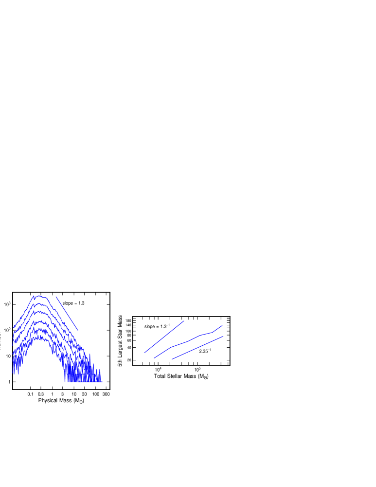
Figure 1: Model IMFs with different numbers of stars showing an increase in the maximum stellar mass with increasing number of stars. The figure on the right shows the mass of the fifth largest star versus the total stellar mass, with an expected slope equal to $1/x=1/1.3$ and a measured slope equal to $\sim 1/2.35$.

An IMF model based on random sampling from a hierarchical cloud (Elmegreen 1997a) shows this effect clearly in figure 1. Each curve on the left is from a different cluster, with a number of stars in the clusters equal to 2500, 5000, 10000, 25000, 50000, and 100000. As the number of model stars increases, the mass of the largest star increases too, as shown on the right of the figure. The expected slope of the power law relation between cluster mass, $M_{cl}$, and maximum star mass, $M_{max}$, is $1/x$, i.e., $M_{max}\sim M_{cl}^{1/x}$; actually the calculation gives a slightly steeper slope because of storage limitations to the number of hierarchical levels allowed in the simulation (these models use 8 levels with an average of 3 subclumps per clump at each level). This property of increasing maximum star mass with cloud mass should not depend on any specific IMF model or on the star formation process.

To be more precise about the stochastic interpretation of this effect, we can consider an IMF $n(M)dM=n_{0}M^{-1-x}dM$, which gives the Salpeter function when $x=1.35$. The largest star, with mass $M_{max}$, typically satisfies $\int_{M_{max}}^{\infty}n(M)dM=1$. This gives $n_{0}=xM_{max}^{x}$. Because the total cluster mass is $M_{tot}=\int_{M_{min}}^{M_{max}}Mn(M)dM$, the largest star is related to the total cluster mass as

$$M_{tot}={{x}\over{x-1}}M_{max}\left[\left({{M_{max}}\over{M_{min}}}\right)^{x-1}-1\right].$$ (1.1)

For $M_{max}\sim 10M_{min}$ and $x=1.35$, this gives $M_{tot}\sim 4.8M_{max}$, and for $\left(M_{max}/M_{min}\right)^{0.35}$ $>>1$, this gives $M_{tot}\sim 3.9M_{max}^{1.35}/M_{min}^{0.35}$. Thus, a cluster requires several hundred M_⊙ before a small O-type star is likely to appear, and a cluster with $10^{3}$ M_⊙ is likely to contain $\sim 10$ modest O-type stars or a few very massive ones. This is the mass range for the largest open clusters in the Milky Way disk, indicating that when a few O stars appear, a cluster is likely to terminate its formation in an unbound state, presumably as a result of rapid cloud destruction, and make an expanding OB association (Elmegreen 1983).

Larson (1991, 1992) and Khersonsky (1997) interpret this observation in the opposite way, saying that there is a physical effect which tends to produce higher mass stars in clouds of higher mass, and that the IMF partly results from this physical effect. Larson (1992) attributes the physical effect to a larger accretion length in larger clouds for material going into a star. If there is such an effect, and the observation is not entirely statistical as discussed above, then the superposition of IMFs from clouds of different mass would be different from the IMF in any one cloud. That is, clouds of low mass would produce an IMF with a particular slope up to some maximum mass, and clouds of higher mass would produce an IMF, perhaps with the same slope, up to higher masses. The sum of these two IMFs would be an IMF with greater slope than either separate cloud, because the summed IMF contains low mass stars from both clouds, but only high mass stars from the more massive cloud. Larson (1991) proposed his model by saying, in effect, that only one star forms in each cloud fragment at each level in the hierarchy, and that the star mass is always proportional to the square root of the fragment mass. Then the sum over all fragments is the final IMF, and this has a slope of $x=2$, which is not too bad. Stated this way, there is no problem with the model because each component in the sum is only a single star, not a whole cluster of stars with a separate IMF. However, even in this model, if we add together the stellar populations from many separate clouds with different total masses, then the summed IMF will be steeper than the IMF in each. At this point, it is important to recall that the IMF obtained from large-scale surveys of galaxies and their metallicities is about the same as the IMF observed in individual clusters. Thus the summed IMF from many regions of star formation has to be about the same as the IMF from each separate cluster. This would seem to suggest that the observed increase in maximum star mass with cloud mass is not the result of a physical process that specifically increases the upper stellar mass in larger clouds.

A second peculiarity about star formation is that the high mass stars tend to form after the low mass stars (Herbig 1962a,b; Iben & Talbot 1966). This has been determined most recently for 30 Dor (Massey & Hunter 1998). Again one can think of physical reasons for this, such as a gradual warming of the cloud following the formation of low mass stars, and an increase in the Jeans mass with temperature (Silk 1977; Yoshii & Saio 1985), but statistical effects can explain it too.

The decreasing nature of the IMF at high mass implies that massive stars are likely to form only after a lot of low mass stars have already formed. For a constant star formation rate, the average time between the formation of stars in a logarithmic mass range centered on $M$ is proportional to the rate at which these stars form, which is inversely proportional to the relative number of the stars, or $\left(Mn[M]\right)^{-1}\propto M^{x}$. For a constant star formation rate, this is also the average time after star formation begins for the first appearance of a star with this mass. Thus the most common, low-mass stars form first, followed by the intermediate and then the high mass stars. In terms of the proportion of all stars formed, and for a constant star formation rate in units of mass per year, the maximum stellar mass increases with time as

$$\int_{M_{min}}^{M_{max}(t)}Mn(M)dM=At$$ (1.2)

for star formation rate $A$. Thus, a star of mass $M(t)$ forms after the proportional time given by

$${{t}\over{t_{max}}}={{\int_{M_{min}}^{M(t)}Mn(M)dM}\over{\int_{M_{min}}^{M_{max}}Mn(M)dM}}.$$ (1.3)

For the power law portion of the IMF only, with $M_{min}=1$ M_⊙ and $x=1.35$, this becomes, for masses in M_⊙,

$${{t}\over{t_{max}}}={{1-M(t)^{-0.35}}\over{1-M_{max}^{-0.35}}}.$$ (1.4)

For example, in a cluster with a maximum stellar mass of 30 $M_{\odot}$, stars with 10 M_⊙ form in the last 20% of the time.

Note that this increase in time with stellar mass is only for the first appearance of a star with that mass. The average time of appearance is independent of stellar mass in the stochastic interpretation. This suggests a way to check the stochastic model of birth orders. If the average time of appearance of all stars with mass $M$ is the average age of the cloud, and this is true for any $M$, and if the first time of appearance of a star with mass $M$ increases with time, as described above, then the birth order is dominated by stochastic effects.

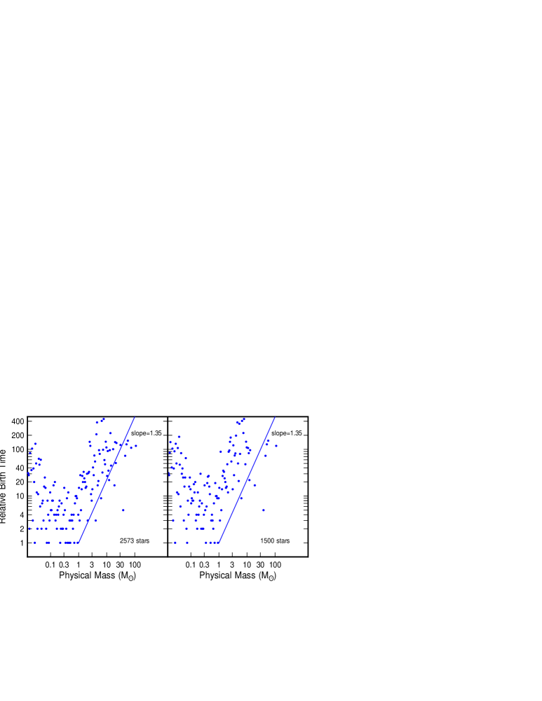
Figure 2: The relative birth time for the first appearance of a star with a certain mass is shown as a function of mass for a composite of 11 clusters on the left, containing 2573 stars total, and 6 clusters on the right, containing 1500 stars. The relative birth time is measured in units of the time of first appearance of any star in the model. The solid line has a slope of 1.35.

Figure 2 shows the relative birth order of stars in the random sampling IMF model by Elmegreen (1998). Each point marks the earliest time of formation of a model star with that mass, among all of the stars that formed in 11 clusters on the left and 6 clusters on the right. Each cluster contains 200 to 500 stars and is independently generated. The plot shows a distribution of points that traces the inverse of the IMF in log intervals. The fiducial line has a slope of $1.35$ for comparison. The increase at low mass occurs because the model uses a Gaussian probability for failure to form a star at low mass, which is an arbitrary assumption at this time (it causes the model IMF to turn over at low mass).

There are no quantitative measures yet of how the earliest appearance of a star with a particular mass increases with time relative to the birth order of all stars, so the predictions of theory cannot yet be checked. In a real star-forming region, the star formation rate is probably not constant in time, so the ordinate in figure 2 should not be time, but star number in its proper birth order; i.e. one should plot, for the first appearance of a star of mass $M$, its mass versus the number of stars that formed before it.

An interesting implication of the above two discussions is that massive stars must not be able to severely limit or halt star formation in their primordial clouds. If they did, then, considering their relatively late appearance, each cloud would produce stars with the same local IMF up to some maximum stellar mass at which point the cloud is finally destroyed. This maximum stellar mass at the time of cloud destruction is presumably larger for more massive clouds, because it is harder to destroy a massive cloud than a low mass cloud. Thus the summed IMF from many regions of star formation would be steeper than the local IMF in each region, for the reasons discussed above, and we could not explain why the integral IMF in a galaxy is the same as the cluster IMF. Perhaps massive stars only shred the low density parts of these clouds, allowing (or perhaps stimulating), most of the cores that have already formed in these regions to continue their evolution toward stars. In view of this, it seems that stars of all mass are probably equally likely to form in any cloud (that contains at least this much mass), regardless of what other stars have formed before them. Moreover, the maximum stellar mass is not physically limited, it is only statistically limited in the sense that extremely massive stars are rare. An exception to this conclusion may arise in the “field” population studied by Massey et al. (1995b), in which the summed IMF of presumed dispersed clusters appears to be steeper than the IMF in each. Maybe massive stars can more easily disrupt their clouds in low pressure “field” environments. On the other hand, maybe the Massey et al. observation can be explained in other ways.

A third peculiarity of the IMF is that massive stars are often closer to a cluster center than low mass stars. This effect has been discussed for a long time (e.g., Sagar et al. 1988), but it was never certain whether the observations reflected a birth position, or just a relaxation effect after the cluster formed. Thermal relaxation makes the high mass stars sink to the center of the cluster, on average, in a thermalization time scale. However, Hillenbrand & Hartmann (1998) and Bonnell & Davies (1998) have recently shown that this peculiar mass distribution, which is observed in the Trapezium cluster, could not result from thermalization because the Orion cluster is too young (see also Jones & Walker 1988). Similar mass segregation has been observed in NGC 2157 (Fischer et al. 1998). Thus it is an effect that should be explained by an IMF theory, and it is likely to result from a physical process during star formation rather than stochastic sampling.

There have been many attempts to explain this relative birth position (see reviews in Larson 1991, and Zinnecker, McCaughrean & Wilking 1993), including excess gas clump collisions in the center of a cloud (Larson 1990; Stahler, Palla, & Ho 1998), excess gas accretion onto protostars in the cloud core (Larson 1978; Larson 1982; Zinnecker 1982; Bonnell et al. 1997), enhanced gas drag for massive protostars (Larson 1990, 1991), late-time formation of high mass stars in a collapsing cloud (Murray & Lin 1996), and hierarchical cloud structure in which the massive trunk of a hierarchical tree for the gas cloud is closer to the center of the tree than the low-mass branches (Elmegreen 1998). A combination of these effects might be involved.

1.4 Summary

There are evidently four distinct physical effects that have to be explained by a theory of the IMF:
(1) the power-law slope at intermediate to high stellar mass, with a value close to that found by Salpeter (1955);
(2) the flattening at low mass for clusters and star-forming regions in our Galaxy;
(3) the increase in the transition mass between power-law and flat regions of the IMF in starburst galaxies,
(4) the preferential birth of high mass stars close to cluster centers.

There are apparently three additional observations that can be explained by stochastic sampling effects:
(1) the tendency for the largest mass star in a region to increase with the total number of stars;
(2) the tendency for the largest mass stars to form last, and
(3) the seemingly random variations in the intermediate and high mass IMF slopes from region to region, along with the appearance of gaps, ledges, and other peculiar departures from a power law.

In addition to these observations, there are tentative indications that other IMF features may be present, including:
(1) a turnover at low mass, and
(2) a steepening of the power-law part in field regions.
Future observations should be able to illuminate these uncertain features.

2 What Determines a Star’s Mass?

2.1 A Steady Stream of Theories

The theory of the IMF depends on both the theory of star formation and the theory of cloud structure. Because of the complexity of these issues, the IMF may not be understood for a long time. Here we review some recent developments. Previous reviews were in Cayrel (1990) and Clarke (1998).

One of the key problems in understanding the origin of the IMF is to determine the processes that limit the pre-stellar gas accretion onto a star and define the star’s final mass. There have been several ideas on this.

The final mass could result from the star’s own ability to limit the accretion of new gas onto its surface, perhaps because of an intense proto-stellar wind (Larson 1982; Shu, Adams, & Lizano 1987), which is known to exist at this phase of evolution (Lada 1985). This possibility has led to several theories of the IMF. One, proposed by Nakano, Hasegawa, & Norman (1995), considered three mass-limiting agents: protostellar winds, ionization, and depletion of the gas clump in which the star forms. They concluded that under normal conditions, the protostellar wind would limit the accretion. Then they calculated the fraction of the clump that would get into the star, finding that the final star mass scaled with the clump mass to the $7/6$ power. To get an IMF slope of $x=1.7$, which they got from the field-star IMF in Scalo (1986), they required a very steep clump mass spectrum, $n(M_{clump})\sim M_{clump}^{-3}$ in linear intervals, instead of the usual observation of $M_{clump}^{-\alpha}$ with $\alpha\sim 1.5-1.8$ (Blitz 1993; Kramer et al. 1998). They justified this steep clump spectrum by noting that if the linewidths found in a CS survey of Orion clumps (Tatematsu et al. 1993) were assumed to be virial velocities, and the masses calculated accordingly, then the Orion CS clumps would have such a spectrum.

Another IMF model with wind-limited stellar masses was proposed by Adams & Fatuzzo (1996). They conjectured that the stellar luminosity scales with the wind mass loss rate, which, at the time when the accretion stops, is proportional to the direct accretion rate onto the star, independent of what goes onto the disk. This gave them a relation between the stellar properties, i.e., luminosity and mass, and the gas cloud properties, sound speed and angular rotation rate. The angular rotation rate entered because they had to determine the fraction of the accreting gas that goes into the star and not the disk. Finally, they related the stellar mass to the total luminosity of the star, from the sum of the accretion-driven luminosity, which depends on mass, and the luminosity of a main sequence star at intermediate mass, from the standard mass-luminosity relation. The result is a relation between stellar mass and the cloud properties, i.e., sound speed and rotation rate. Taking the mass distribution for clumps with the observed slope $\alpha$ discussed above, and the empirical relationship between clump mass and velocity dispersion from Larson’s (1981) laws, they got a distribution function for the clump velocity dispersion, which then led to a distribution function for the final star mass if the angular rate of all the clumps is the same. Adams & Fatuzzo (1996) also discussed more general equations giving the stellar mass from cloud properties, considering random variations in these cloud properties, and derived a log-normal final mass distribution, as in Larson (1973), Elmegreen & Mathieu (1983), Zinnecker (1984), and Elmegreen (1985).

Silk (1995) also got a relation between cloud core mass and turbulent linewidth, different from Adams & Fatuzzo’s, considering centrifugally supported cores with luminosities equal to the accretion luminosities. He considered an equality between the turbulent linewidth and the thermal velocity in the core, which entered into the luminosity through the temperature using the usual radiative transfer equation for a star and the Rossland mean opacity. Then, after substituting the empirical correlations between clump rotation rate and size, and between linewidth and size, he got the cloud core mass as a function of the turbulent linewidth. The distribution function for cloud core mass then followed from a distribution function for linewidth, which came from a theory for the time-dependent deceleration of wind-driven bubbles in a cloud. The star mass is then taken to be proportional to the cloud core mass. Silk (1995) made several comments that protostellar outflows limit the mass of a star, but this assumption was not present in any of the theory in his paper, nor in the IMF that resulted, particularly considering that a fixed fraction of the cloud core mass was assumed to go into the star. This was unlike the results of the wind-limited accretion models proposed by Nakano, Hasegawa, & Norman (1995) and Adams & Fatuzzo (1996).

One of the most popular and persistent methods for determining the mass of a star has been with a combination of cloud fragmentation, accretion, and clump collisions. Larson (1978) showed with three-dimensional N-body experiments that gas clouds fragment hierarchically by self-gravity, and the fragments accrete material in competition with each other. The resulting mass distribution was modeled after a fractal, which was a remarkably prescient concept in astronomy considering that Mandelbrot (1977) began to popularize his fractal geometry only a year earlier. Larson showed that the fractal mass function would have a slope of about $x=1$, in reasonable agreement with observations. Larson also reasoned that the lower mass limit to a star is the thermal Jeans mass in the cloud because smaller condensations are not likely to form in the initial collapse. This experiment was an important departure from standard fragmentation models of the time, since it was previously believed, following Hoyle (1953) and Hunter (1962), that fragmentation decreased the Jeans mass, leading to ever more fragmentation. In Larson’s result, the number of clumps formed was about equal to the number of Jeans masses in the initial cloud, with no subfragmentation into smaller pieces. This result was seconded by Tohline (1980), but investigated again by Silk (1982), who concluded that initial cloud fragments, particularly elongated fragments, formed by dynamical collapse could in fact fragment again (see also Bonnell & Bastien 1993, Burkert et al. 1997).

Silk (1977) considered a different picture of cloud fragmentation, using a thermal Jeans mass that increased with time as a result of heating from the stars that already formed. His model of fragmentation was simpler than Larson’s, so there was no built-in, power-law mass spectrum from the fragmentation process itself. The power law in Silk’s model came from the time increase in the thermal Jeans mass and the identification of this mass with the stellar mass at all times. Yoshii & Saio (1985) followed this model by considering the additional influence of coalescence among the opacity-limited fragments. They showed that the opaque fragments are usually so small that coalescence is unimportant; thus fragmentation and heating alone determine the IMF as a time sequence of increasing thermal Jeans masses, as in the Silk (1977) model. Bastien (1981) obtained a different result by using the Jeans length to determine the fragment collision cross section. The initial Jeans length is much larger than the size of the opaque fragments considered by Yoshii & Saio (1985), so Bastien (1981) found that fragment collisions were important. Subsequent work by Lejeune & Bastien (1986), and Allen & Bastien (1995, 1996) considered time-dependent coalescence, and concluded again that both fragmentation and coalescence were important, with coalescence dominating the formation of massive stars.

Price & Podsiadlowski (1995) used protostar collisions in a different way. They proposed that stars grow by accretion at some more-or-less uniform rate, and this accretion stops when two protostars collide, disrupting the gas reservoirs from each. The final stellar mass was then determined by the product of the accretion rate and the time interval between collisions. The IMF was built up over time as the final stellar mass decreased in the presence of an increasing collision rate that resulted from the continuous formation of more and more protostars.

Another coagulation model was proposed by Murray & Lin (1996). They suggested that fragmentation driven by thermal instabilities leads to clumps that fall in the potential well of a cloud, after which they collide and coalesce with other clumps that have fallen too. A star forms when the clump mass exceeds the thermal Jeans mass, although further coalescence can increase that mass afterwards. The power-law distribution of masses follows from the coagulation process, in a manner similar to that proposed by Silk & Takahashi (1979). There is no assumption about wind-limited accretion here; the star mass is identified with the core mass directly. An interesting aspect of their model is that they considered positionally correlated velocities, as in a turbulent fluid, but they showed this had no important effect on the model IMF.

Numerical SPH simulations of an evolving IMF made of accreting, pseudo-star particle clumps was done by Bonnell et al. (1997). The advantages of numerical solutions like this is that they can treat well the competition for gas among all the nucleated centers. They found that nucleating centers originally close to the center of the whole cloud grow faster and to larger masses because of the larger gas density there.

2.2 An IMF from Random Selection of Mass in Hierarchical Clouds

A different class of theory considers only the statistical aspects of the IMF. The Hoyle (1953) picture of fragmentation led naturally to these ideas, because successive fragmentation produces hierarchical structure and power law mass spectra regardless of many physical details. Larson (1973) considered a modification to these ideas by proposing that only part of each fragment undergoes further fragmentation, and got from this a log-normal mass distribution instead of a power-law. When Miller & Scalo (1979) proposed that the IMF actually had a log-normal form, the statistical implications of this were developed further by Elmegreen & Mathieu (1983), Zinnecker (1984), and Elmegreen (1985), who showed that a variety of processes, acting together, would combine to make a log-normal function, regardless of the distribution functions resulting from each separate process. This point was made again more recently by Adams & Fatuzzo (1996).

The most recent development in this area has been by Elmegreen (1997a, 1998), who considered the random selection of masses from a hierarchically structured cloud. These papers depart from the usual scenarios by asserting that hierarchical cloud structure is independent of star formation – that it is set up long before star formation begins in the diffuse cloud stage, and then continuously reestablished during the molecular cloud stage as a result of supersonic turbulence compression. There is no gravitationally-driven fragmentation at all, and no significant clump coalescence. In fact, the clumps in this model need not even be constant objects, able to move around and coalesce; they can be ever-changing gas compressions and wavepackets in the chaotic turbulent flow. This model is motivated by the pervasive appearance of hierarchical structure and spatially-correlated velocities in interstellar clouds. These features are reminiscent of structures and flows in laboratory turbulence (e.g., see reviews in Sreenivasan 1991, and Falgarone & Phillips 1991).

The basic point of the Elmegreen (1997a, 1998) model is that essentially all local star formation processes that have been considered in detail have a time scale for evolution that varies approximately as the inverse square root of local density, including contraction or collapse from self-gravity, turbulence compression, magnetic diffusion in virialized cores, and coalescence at each level in the hierarchy. This means that in a model like this, stars will appear here and there, randomly, alone or with neighbors, at a rate that depends almost exclusively on the local square root of density. On a large scale, this implies that dense clouds in high pressure regions of galaxies will form all of their stars quickly, while low density clouds in low pressure regions will take much more time. On a small scale, within any one cloud, it means that different parts of the hierarchy form stars at different times. The density always increases at lower levels in a hierarchical structure, and this is where the clumps, contained by other clumps on larger scales, are small and have low mass. Thus the low mass pieces in a cloud are likely to form stars first. As a result, there is slightly less mass for other stars that form later in the same or higher levels. This competition for mass tends to steepen the power in the power-law mass function by several tenths, i.e., from $x=1$ to $x=1.35$, as in the Salpeter IMF.

Perhaps a more important difference in this new model is the way in which cloud structure is measured. Typically, the power law index for molecular and diffuse cloud structure is determined from the mass distribution of separate clumps, resolved in large-scale surveys by various telescopes and then separated into discrete objects either by eye or by computer algorithms that do about the same thing as the eye. These mass distributions are always much flatter than the IMF, having slopes $\alpha$ in the range from 1.5 to 1.8, when the IMF has a slope of about $1+x=2.35$. To understand the IMF, however, we have to try to view interstellar clouds from the perspective of a forming star. A star does not care about the clumps that our telescopes resolve and our eyes choose to label as discrete, but only about the general distribution and motion of gas in all forms. In pre-star-forming clouds, where this structure is first established, it is largely hierarchical, from scales that are much smaller than mm-wave telescopes can resolve, up to perhaps a galactic scale height.

Hierarchical means that most of the small clouds are contained inside larger clouds, and most small stellar groupings are inside larger stellar groupings (see review in Elmegreen & Efremov 1998). For example, Efremov (1995) and colleagues have estimated that 90% of the OB associations in the Milky Way (Efremov & Sitnik 1988), M31 (Efremov, Ivanov, & Nikolov 1987; Battinelli 1991, 1992; Magnier et al. 1993; Battinelli, Efremov & Magnier 1996), M33 (Ivanov 1987, 1992), and the LMC (Feitzinger & Braunsfurth 1984) are inside larger star complexes. Scalo (1985) has reviewed hierarchical structure for interstellar clouds. It appears as if the hierarchical embedding of interstellar and young stellar structures is nearly all-inclusive.

Emission line surveys leading to “discrete” clump masses do not consider this aspect of cloud structure. If two clumps are close together and part of a larger structure, the algorithms call them two separate objects, and do not tabulate the larger “object” that contains them. For this reason, all emission line or extinction surveys catalogue clouds that are within a factor of $\sim 3$ to 10 of the angular resolution, regardless of the cloud distance or the wavelength of the observation. This factor of $3-10$ for recognized clump size corresponds to a factor of $\sim 100$ for cloud mass (which scales as the size squared or cubed in CO surveys), so the mass functions look reasonably well sampled, but in fact only a small part of the cloud structure is included. Everything smaller than the telescope resolution is not seen, and everything larger than about 3 to 10 resolution elements is subdivided into its component parts and not called a separate object. This is how every cloud or clump mass function has been evaluated since the beginning of this exercise (i.e., since before Field & Saslaw 1965).

The Elmegreen (1997a, 1998) model takes a different point of view. It considers the structure on all scales and asks for the probability that any particular mass is chosen from anywhere in the whole hierarchy. This is presumably what happens as a result of the combination of physical processes that leads to star formation in a real cloud: because of the self-similar nature of turbulent flows, each level in the hierarchy looks the same as any other level (for masses above the thermal Jeans mass), so each choice of level for a star-formation event would have the same likelihood as any other choice, modulated only by the density-dependent local evolution rate discussed in the previous paragraph. Aside from this variable rate, the instantaneous distribution of masses for all structures, and the instantaneous probability of selecting any particular mass, is proportional to $M^{-2}$ for linear intervals in mass (i.e., $\alpha=2$ in the notation of the clump spectra given above). Such a distribution for hierarchical structure was also recognized by Larson (1978) and Fleck (1996). The result gives a steeper instantaneous mass function than emission line or extinction surveys, but there is no conservation of mass as in these standard surveys (i.e., the sum of the masses of all possible structures is larger than the mass of the whole cloud, because nearly all of the structures are contained in other structures, and so are multiply counted). This way of viewing cloud structure seems to be closer to what a real star-forming process “sees” before it actually begins the sequence of events that makes a star. The density dependent rate of star formation then steepens the mass function from $M^{-2}$ to $M^{-2.35}$. This result is then identified with the Salpeter IMF.

For the purposes of understanding the IMF, there are probably better ways to measure cloud structures than with clump-finding algorithms. The structure on the edges of clouds has been analyzed in terms of fractals, rather than clumps, for many years (Beech 1987; Bazell & Désert 1988; Scalo 1990; Dickman, Horvath, & Margulis 1990; Falgarone, Phillips, & Walker 1991; Zimmermann & Stutzki 1992, 1993; Henriksen, 1991; Hetem & Lepine 1993; Vogelaar & Wakker 1994; Pfenniger & Combes 1994).

For the structures inside clouds, Stutzki et al. (1998) showed that Fourier transform power spectra of emission line intensity scans across molecular clouds gave power laws, and concluded that the internal structure was scale-invariant, as in a fractal. They reproduced this structure with a random fractal-generation model. Other models that made cloud fractals were in Hetem & Lepine (1993) and Elmegreen (1997b). The concept that the cloud mass distribution function is the result of fractal structure, presumably generated by turbulence, began with papers by Fleck (1996), Elmegreen & Falgarone (1996), and Stutzki et al. (1998). This seems to be a more reasonable explanation than the older collisional-build-up models of clump structure, particularly since off-center supersonic collisions between clumps should not be sticky (Scalo & Pumphrey 1982; Kimura & Tosa 1996; Fujimoto, & Kumai 1997).

The probability of selecting structures for star formation in hierarchical clouds seems to show up more directly in the distribution of masses for open clusters. When a bound cluster forms, a high fraction of the gas mass has to go into stars (see Verschueren 1990 and references therein), so the cluster mass distribution should reflect the mass distribution of cloud structures pretty well. In this case, the result is obviously independent of telescope resolution or cloud-clump recognition bias, because clusters are seen optically, even at great distances. Also, the range of masses for clusters can be reasonably large, exceeding a factor of 100, so a power law can be measured fairly well if it exists. Cluster selection suffers from various other biases, however, such as extinction, age limitations, and a loss of low-mass clusters with increasing distance. Nevertheless, there are some studies that get around these biases, and they confirm the expected result. In two samples of nearby clusters, each with calibrated masses, Battinelli et al. (1994) found power law mass functions with slopes of $-2.13\pm 0.15$ and $-2.04\pm 0.11$. These clusters are close enough to the Sun to be relatively free of distance and extinction effects. Also, in the LMC, where $\sim 600$ clusters are catalogued (Bica et al. 1996), calibrated photometrically for age (Girardi et al 1995), and all at about the same distance, Elmegreen & Efremov (1997) found $M^{-2}dM$ mass functions for discrete age groups (e.g., $10^{8}-10^{9}$ yrs; dividing the clusters into age groups is important when there are no direct measures of cluster mass, because the conversion from luminosity to mass depends on age).

The IMF should be steeper than the cluster mass function because of the density-dependent formation rate of individual stars, and the competition for mass in the IMF. These effects are not important for clusters. Open clusters take a high fraction of all the gas mass originally available to them (or else they would not have ended up bound), and the rate at which they do this is not important for their final masses. In the case of stars, new objects forming at one level steal mass away from the objects that form later at a higher level. But clusters do not do this: those which form inside other clusters in the general hierarchy can just merge together to make a single cluster of higher mass, appropriate to the higher level in the hierarchy. And if they do not merge, then they stay with their original masses, which are appropriate for the levels in which they form.

Other IMF models based on fractal or hierarchical cloud structure were developed earlier by Henriksen (1986, 1991) and Larson (1992). Henriksen used the size, $L$, distribution function of structures in a fractal of dimension $D$, given as $n(L)d\log L\propto L^{-D}d\log L$ by Mandelbrot (1983), and assumed that the density $\rho$ varied with size too, not as in a fractal (which would be $\rho\propto L^{D-3}$) but as actually observed in self-gravitating clouds, namely $\rho\propto L^{-1}$. This gave a mass function for cloud structure that agreed well with observations if $D\sim 2.7$. Note that if Henriksen used the density dependence for a fractal, in a self-consistent manner with the size distribution, then the resulting mass function would have been independent of the fractal dimension, $M^{-2}dM$, as discussed above for hierarchical clouds in general. Larson (1992) started again with the size distribution for a fractal, and assumed that final stellar mass is directly proportional to the linear size of the cloud structure, suggesting that such structures were filamentary anyway. Then the slope of the IMF in linear intervals became $1+x=1+D\sim 3.3$ for $D=2.3$, as implied by the fractal dimension of cloud perimeters, namely $D_{p}\sim 1.3$, added to 1 to account for the higher dimension of the surface. This IMF, with a slope of $1+x=3.3$, is significantly steeper than the Salpeter IMF, with a slope of $1+x=2.3$, but Larson suggested that maybe stars form in subparts of clouds where $D$ is smaller than 2.3, or perhaps larger structures have larger temperatures, which would break the assumed linear relationship between star mass and scale size.

These models differ from the Elmegreen (1997a, 1998) model, even though both employ “fractal” cloud structure, because the latter uses general cloud shapes, not necessarily filaments or sheets, random sampling from all levels in the hierarchy of structures (giving $M^{-2}dM$ from sampling alone), a density-dependent rate that steepens the IMF by preferred sampling at lower mass (i.e., steepening the result to $M^{-2-0.5+1.5/D}\sim M^{-2.15}$), and a competition for mass, which steepens the IMF further, to $M^{-2.35}dM$, as in the Salpeter IMF. With these different assumptions, the IMF in the Elmegreen model hardly depends on the fractal dimension at all; it enters into the exponent of the IMF power law as approximately $0.5-1.5/D$, which is a very small increment for $D$ in the likely range of 2 to 3.

2.3 Theories for The Lower Stellar Mass Limit

Understanding the lower mass limit to star formation is an important part of any IMF theory. Various assumptions about this have already been mentioned in the review of theories presented above. Three views on this subject seem to pervade most of them. In the wind-limited accretion models, the assumption is made that accretion onto a dense core continues until a protostellar wind develops, which presumably follows the onset of deuterium burning (Shu et al. 1987). Thus low mass objects do not stay that way very long, they just keep accreting until they become active protostars. In most of the older fragmentation-coalescence models, the minimum mass is the mass of a gravitationally bound fragment that is optically thick. In the various scale-free models, based on gravitationally-driven fragmentation or turbulence, the minimum mass is usually the thermal Jeans mass, particularly in the Larson (1992) and Elmegreen (1997a, 1998) models. This assumption is made because, without further fragmentation during the collapse itself, the thermal Jeans mass is the smallest structure that can ever become self-gravitating, even in the presence of turbulence and magnetic fields.

The first and the third of these mass limits equals about the observed limit, $\sim 0.1$ M_⊙. In the first case, it is self-defining: objects accrete until they become star-like, and then they stop accreting, so naturally the lowest possible mass is the mass of a star. This concept has the powerful advantage over the others that the basic star mass, and perhaps even the IMF itself, can be the same everywhere, independent of cloud conditions. In the third case, the minimum theoretical mass just happens to equal the observed minimum in standard cloud conditions. An expression for this mass is the Bonner-Ebert critical mass,

$$M_{BE}=0.35\left({{T}\over{10K}}\right)^{2}\left({{P}\over{10^{6}\;k_{B}}}\right)^{-1/2}\;\;{\rm M}_{\odot}.$$ (2.5)

Here we have normalized the result to standard cloud conditions, taking the pressure inside a cloud equal to the typical self-gravitating core pressure, not the boundary pressure (which is sometimes lower by a factor of $\sim 30$). Our use of this form for the thermal Jeans mass is motivated by the near constancy of $T$ and total $P$ in molecular clouds, according to the scaling relations (Larson 1981). This is much more sensible than writing the thermal Jeans mass in terms of $T$ and density, for example, when the density varies by several orders of magnitude inside a cloud. Our use of the total pressure for $P$ also allows for a decrease of Jeans mass in compressive flows, as in Hunter & Fleck (1982).

Nevertheless, another theory of the IMF in which all of the stellar masses have the local thermal Jeans mass has been advanced by Padoan, Nordlund, & Jones (1997), with variations in mass entirely the result of variations in the density in a turbulent fluid. In this model, the high mass stars form in the low density regions, because the Jeans mass is high there for a given temperature.

The second minimum fragment mass discussed above, from the opacity limit of a self-gravitating condensation, is typically much smaller than the minimum star mass, so coalescence has to bring the star mass up to the observed value in these models.

Larson has looked for signatures of the thermal Jeans mass in several ways, predicting that it should vary with cloud temperature (Larson 1985, 1992). In Larson (1992), he suggested that such variations were observed by Myers (1991) in different molecular clouds. Larson (1995) also suggested that the length scale at a break in the separation distribution for T Tauri stars was the Jeans length (see also Simon 1997; but see Bate, Clarke, & McCaughrean 1998 and Nakajima et al. 1998 for other interpretations.)

Elmegreen (1997a, 1998) considered $M_{BE}$ from a different point of view, stating that most star-forming regions in normal galaxies actually do have nearly constant values of $T^{2}/P^{1/2}$, with small variations in this quantity possibly leading to the observed variations in cluster IMFs at low mass (see Section 1.1 above). This constancy is a result of the numerator in $M_{BE}$ being approximately proportional to the cooling rate per unit mass of molecular gas (Neufeld, Lepp, & Melnick 1995), and the denominator being approximately proportional to the local surface density of stars and gas in the galaxy, which determine the heating rate per unit mass from cosmic rays and background starlight. As long as cooling roughly balances background heating, this ratio will be about constant. Other, more local variations in $T$ and $P$ tend to cancel out when combined as the quantity $T^{2}/P^{1/2}$. For example, when $P$ goes up in a triggered region next to a previous generation of star-formation, $T$ generally goes up too because of the enhanced radiation field. Conversely, when $P$ is low, as in low-mass clouds like Taurus, then $T$ is low as well.

Elmegreen (1997a, 1998) also points out that the lower mass limit for stars actually does change, perhaps by a factor of 10 in extreme starburst regions (see Sect. 1.1 above) where the average $T$ can be much larger than in local molecular clouds, e.g., 100 K instead of 10 K (cf. Aalto et al. 1995), and the pressure much larger too (e.g., $\times 10^{4}$). But this variation should be rare in normal galaxies because of feedback processes in the interstellar medium that tend to connect young stellar activity, interstellar pressure, and gas temperature. If we consider $T$ to be a measure of the rate of cooling per unit cloud mass, then $T$ in a star-forming region will be high when there is an unusually large embedded or nearby luminosity of stars per unit gas mass. This occurs when the efficiency for star formation is high in a high mass cluster (the cluster has to be fairly high mass to contain the luminous stars that dominate the total radiation field). A high efficiency in a low mass cluster would not necessarily increase $M_{BE}$ because low mass clusters are not very luminous per unit mass. A low efficiency in a high mass cluster, leading to an OB association, might not change $M_{BE}$ much either, because the radiation luminosity per unit gas mass is not particularly large there either. Thus the formation of globular clusters in regions with only moderately large pressures, not the enormous pressures typical of early galactic halos, might be elevate $M_{BE}$, but this conclusion is very uncertain.

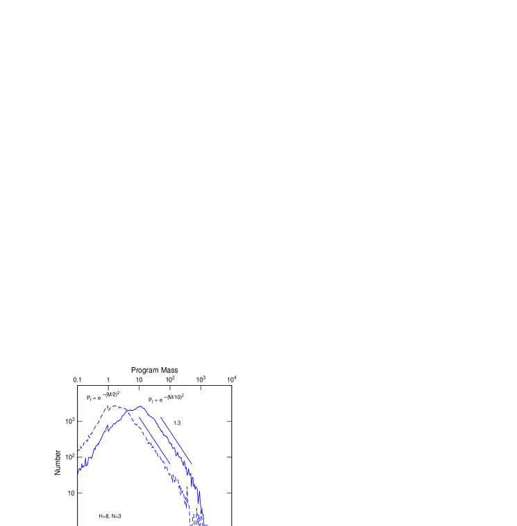
Figure 3: Two model IMFs with different lower mass limits, $M_{BE}$. The entire IMF shifts to the right when $M_{BE}$ increases because the power law portion always has the same slope. The fall-off at high mass is the result of computational limitations. The models have $H=8$ levels in the hierarchy with $N=3$ subclumps per clump, on average.

Figure 3 shows two numerical experiments that made model IMFs from random selections in a hierarchically structured gas cloud, using a rate of selection proportional to the square root of the gas density, as discussed above (Elmegreen 1997a). The models differ only in the value of $M_{BE}$, which enters into the probability for failure to form a star, taken to be $P_{f}=e^{-\left(M/M_{BE}\right)^{2}}$ in these cases ($M_{BE}$ in the figure is written in terms of the computer-program mass, which is scaled to a physical mass after multiplication by $0.15$. The IMFs are identical except for the larger value of the lower mass limit in the case with high $M_{BE}$.

2.4 A Combination of Theories?

The two main contenders for the lower mass limit of star formation, wind-regulation and the thermal Jeans mass, have obvious differences in predicted behaviors of the shape of the IMF at low mass. If this shape varies a lot, with some clusters having clearly higher lower mass limits than other clusters, then wind self-regulation might be ruled out. Moreover, if cluster IMFs in regions with large turnover masses also have larger pre-stellar $M_{BE}$, then the thermal Jeans mass would seem to be important.

Curiously, both of these models, the wind-regulated IMF, and the $M_{BE}$–fractal cloud model, have their strong points where the other is weakest. The wind-regulated IMF model seems to have difficulty explaining the nearly universal slope of the IMF without some sensitivity to cloud parameters, yet it seems certain that wind self-regulation must play some role in determining the mass that gets onto a star, at least near the lower mass limit for star formation. Similarly, models that rely on $M_{BE}$ have an uncomfortable susceptibility to changes in cloud properties near the lower mass limit, but get the Salpeter slope above this limit with essentially no free parameters. Perhaps a combination of the two models would be better.

There are several ways this could occur. First, the fractal model supposes that a star’s mass can be identified with the mass of some structure in a turbulent cloud, but this is obviously too simple – there is a lot that can happen during star formation that will vary the fraction of the cloud mass that gets into a star. If this fraction is randomly distributed, then the same IMF slope and scatter about that slope result, as shown in connection with figure 5 below, which is discussed in more detail in Elmegreen (1998). If it is not randomly distributed, then the power-law slope could change. But the entire power-law slope is not likely to come from wind-regulation, that would give the slope too great a sensitivity to cloud properties and the randomness of wind-clearing. This means that, perhaps to within a factor of 2 to 5, star mass should really be identified with the mass of the clump in which it forms, i.e., that bigger stars really do form in bigger clumps (Casoli et al. 1986; Myers, Ladd, & Fuller 1991; Myers & Fuller 1993; Pound & Blitz 1995; Motte, André, & Neri 1998; not to be confused with the statistical sampling statement discussed in section 1.1, that bigger stars form in bigger whole clouds). This factor of 2 to 5 may contain all the detailed physics of wind clearing.

Protostellar winds should also play some role in regulating the smallest stars that form. According to the models by Shu and collaborators, as reviewed in Shu et al. (1987), the onset of the wind is triggered by deuterium burning in a young, pre-stellar object. If the object is too small, there will be no wind, and presumably accretion will continue until deuterium burning begins.

This concept combines well with the arguments based on a thermal Jean mass. For example, if $M_{BE}$ is much smaller than the deuterium burning limit, then a large number of small brown dwarfs or Jupiters should form, and these could either leave the cloud in that state, forever drifting as brown dwarfs, or they could accrete more mass over time and end up finally able to start a wind. In the latter case, the effective lower mass limit to the IMF would be the deuterium burning mass, not $M_{BE}$, and the larger masses would follow the fractal mass distribution as before, giving the Salpeter function. On the other hand, if there are a lot of free brown dwarfs, which does not appear to be the case in the Solar vicinity (cf. Sect. 1.1), and if there are also a lot of regions where $M_{BE}$ is low, which does not appear to be the case locally either, then a model with accretion up to a wind-limited mass would not seem to work.

If $M_{BE}$ is much larger than the deuterium burning limit, then large, self-gravitating clumps will form in the cloud, but the rapid onset of a wind in these clouds might limit the gas mass that actually gets into the star to only a small fraction of what is available. Then all of the excess mass between the deuterium limit and M_BE would get dispersed back into the cloud for recycling into other stars, and the lower mass limit would be the deuterium limit. In this second case, the mass fraction that goes into each star will be small, but if it is about the same fraction for all clumps, then the higher mass stars will still map out the fractal properties of the cloud and produce the Salpeter IMF. Again the details of how the IMF gets established in a cloud depend strongly on unknown processes during the final collapse and dispersal phase of star formation, but the basic shape of the IMF could be relatively independent of these details.

2.5 Reflections on the Various Theories of the IMF

There have been some fundamental changes lately in how we view molecular clouds and star formation, and these changes inevitably affect the various models for the IMF.

For example, we are beginning to think that star formation is relatively rapid in cloud cores, occurring in only one or two crossing times regardless of scale (Elmegreen & Efremov 1996; Efremov & Elmegreen 1998). This means that we cannot generally wait for magnetic diffusion to occur as a cloud core slowly accretes across field lines. Diffusion typically takes about 10 free fall times for cosmic ray ionization (Shu et al. 1987), longer for ionization by starlight (Myers & Khersonsky 1995), and longer still if the gas is clumpy (Elmegreen & Combes 1992). Indeed, Nakano (1998) suggested that all star-forming cloud cores are magnetically supercritical; i.e., they would collapse dynamically across the field lines if turbulent motions were not present.

There are two important implications of this change in thinking, if correct. First, there would no longer be a strong motivation for IMF theories that consider bimodel star formation in the sense that low mass stars come from subcritical cores, and high mass stars come from magnetically supercritical cores (Lizano & Shu 1988). The IMF is so remarkably uniform anyway, it does not seem possible to have widely different modes of star formation at high and low mass. Any change from low mass dominance to high mass dominance in the IMF could more easily be accommodated by an upward shift in the thermal Jeans mass (cf. Section 2.3).

Secondly, this time scale for star formation may be too short to allow multiple interactions between protostellar clumps. This would then rule out a broad class of coalescence and slow accretion models. Such coalescence is unlikely anyway for clumps that move supersonically relative to each other; they will fragment or disperse upon collision, rather than stick together. Clump collisions may trigger star formation when they occur (Bhattal et al. 1998), but multiple collisions are probably not the source of the cloud or star mass distributions.

Another observation that suggests the same thing is the extremely high stellar densities in young globular clusters, which form today in starburst regions. As suggested in Section 1.1, these globulars look like they will evolve into objects similar to our Milky Way’s halo globulars, and the old Milky Way globulars have an apparently normal IMF. If coalescence is important in local “normal” embedded clusters, it would seem to be devastating in globular clusters, where the stellar density can be $10^{4}$ times higher. Conversely, if these globulars have normal IMFs, then protostellar coalescence must be unimportant nearly everywhere. A similar constraint would come from the IMF in small regions, where only a few stars form. There, protostar interactions are not likely to be important either.

A second major shift in our view of molecular clouds is that most astronomers now think that pre-stellar structure comes from turbulence, not gravitationally-driven fragmentation. This is because the same character of structure is observed in both self-gravitating and non-self-gravitating clouds, and both types of clouds have correlated motions reminiscent of laboratory turbulence. A related point is that the cloud cores in which clusters form are not obviously collapsing as a whole: there are no inverse P-Cygni profiles indicative of collapse motions for whole cores, as there are in some individual protostars. The stars are apparently forming inside more-or-less stable cloud cores. Once again, the general collapse models seem untenable.

The presence of supersonic turbulence also seems to rule out models involving thermal instabilities. Turbulent motions in cluster-forming cores are generally much larger than thermal, and so the dominant forces that structure the gas are the turbulent forces, not the thermal. This means that turbulence causes the observed structures in pre-stellar clouds, not thermal instabilities. Thermal processes are probably important on the smallest scales, but these are at and below $M_{BE}$.

Turbulence in pre-stellar clouds also appears to generate structure that is much lower in mass than even the smallest stars, perhaps as low as $10^{-4}$ M_⊙ (Heithausen et al. 1998; Kramer et al. 1998). This means that star formation occurs in the middle range of all cloud structures, not at the bottom end. It also means that, while turbulence may generate a cascade of structures down to smaller and smaller scales, the end result of this cascade is not the formation of a star. Turbulence makes cloud structures independent of star formation. Self-gravity, sonic wave generation, magnetic reconnection, and many other aspects of interstellar cloud dynamics are likely to be important too by the time star formation begins.

2.6 Implications of a Nearly Uniform IMF

The remarkable near-uniformity of the IMF in regions with a wide range of stellar densities, cluster masses, metallicities, ages, and galactic types strongly suggests there is a unifying process in star formation that makes the relative probability of forming various masses somewhat independent of physical parameters. For example, the IMF seems independent of how star formation begins, i.e., whether the region is triggered by some external pressure or forms quiescently (e.g. see Parker et al. 1992 and the contrary opinion by Oey & Massey 1995), independent of the general cloud shape (shell, layer, filament, etc.), magnetic field strength, ionization level, presence of other stars, and so on. This is remarkable because these physical variables do control the rate of star formation in some regions, and they certainly control where and when star formation begins. They just do not appear to influence the IMF.

The near-uniformity of the slope of the power law also implies several other things. (1) There is a universal aspect of cloud structure and evolution that produces the power-law portion of the IMF independently of the temperature, pressure, and metallicity. This means that the power-law probably does not depend on the protostellar collapse process, e.g., on the fragmentation or collapse of isothermal clumps, the accretion of gas in thermal equilibrium, or the thermal Jeans mass. For all of these processes, thermal temperature and magnetic diffusion are probably important at some stage (see reviews in Nakano 1984; Mouschovias 1991; Shu, Adams, & Lizano 1987). (2) The IMF power-law is also likely to be a highly reduced average over many physical processes that either all give about the same result, or are combined so finely in every region that the same proportion of each process is always present.

The variations in slope of the IMF from region to region (Scalo 1998) seem at first to suggest something different, that the IMF is not in fact uniform but depends sensitively on physical conditions. But are these variations statistically significant? Rarely do studies of cluster IMFs contain more than several hundred stars.

Figure 4: (top left) IMF slopes in 100 models, plotted as a function of the average logarithm of the mass. Each IMF slope is fit using 200 stars, with the largest star in the fit taken to be smaller by 20 filled mass bins than the largest star produced in the model. The Salpeter value of $-1.35$ is shown by a dashed line. The three values indicated by crosses have their complete IMFs shown in the other panels. The fitted portions of these IMFs are indicated by the offsets.

Figure 4 shows sample IMFs from the model of random selection in a hierarchical cloud (Elmegreen 1998). The panel in the upper left shows IMF slopes for 100 different models, each with a different number of stars and therefore different upper mass limit. In all cases, the range of stars chosen for the power-law slope determination is such that there are 200 stars in the fit, starting from the histogram bin that is twenty filled bins (a factor of 3 in mass) away from the most massive star, and going to lower mass bins. This starting point for the fit ensures that there are enough stars to get an accurate slope, and it coincides with an astronomer’s decision to avoid fitting the IMF to the scarce few highest-mass stars in the cluster. We pick a different number of total stars for each IMF, and use only the highest mass parts of each model, because this is what an astronomer would do as well. Generally an observer catalogues only the brightest stars in a cluster and misses the low mass members. If a cluster has an IMF made only from low mass stars, then that cluster is generally so small that there are no high mass stars at all.

Evidently the IMF slope varies a lot around the Salpeter value, shown in the figure by the dashed line at $x=1.35$. This average slope is nearly independent of physical cloud properties in this model (see the discussion in section 2.1). The other three panels in figure 4 show particular IMFs and the mass ranges and fits used for the “X” marks in the top left panel.

Figure 5: The rms deviation in the fitted slopes of the model IMFs for the 1-10 M_⊙ range, plotted versus the number of stars that are included in the fit. The solid line is for the case shown in Fig. 4, and the dashed line is for another 100 independent IMFs that have an additional randomness in the ratio of the star mass to the clump mass.

Figure 5 shows the rms deviations in the IMF slopes around the mean values for power-law fits that include different numbers of stars in the same 100 IMFs (from Elmegreen 1998). Each plotted value, connected by a smooth line, represents the rms deviation for the 100 models, calculated in the mass range from 1 to 10 M_⊙ (the characteristic physical mass in the model comes from $M_{BE}$, which is taken to be 0.35M_⊙ from equation 2.5). The rms deviation around the Salpeter slope decreases systematically as more and more stars are included in the fit. The deviation can be as high as $\pm 0.5$ when only 80 stars are used, decreasing to $\sim 0.1$ when 1000 stars are used. This implies that an IMF calculated with, say, 150 stars, and having a slope of $-1.15$ instead of the Salpeter slope of $-1.35$, is in fact statistically consistent with this Salpeter slope in a “universal” IMF. The fluctuations found by Scalo (1998) in his review correspond to $\pm 0.5$ around the value $x\sim 1.35$. These fluctuations could be statistical, considering the number of stars included in typical IMF surveys and the likely presence of measurement and star selection errors in the real data.

The dashed line in figure 5 is for another 100 models, independent of the first, and evaluated with a large ($\times 4$) and random fluctuation in the ratio of the star mass to the clump mass. Such variations do not affect the average IMF slope or the statistical fluctuations around it.

3 Summary

The IMF has been observed directly and indirectly for many years, with many different results, but there seems to be some convergence now in the basic form of the IMF, and also some tantalizing indications that this form changes a little when the physical conditions for star formation change a lot. The main observational results were summarized in section 1.4.

The theory of the IMF seems to be all over the map, even in recent years. This variation reflects our ignorance in the processes that determine a star’s mass and in the processes that cause the complex spatial structures seen in interstellar clouds. The common aspects in many of these models, including clump and protostellar interactions, wind erosion of protostellar gas concentrations, minimum masses from the lack of self-gravity, and hierarchical cloud structure, are all likely to play some role in generating the IMF. The worry is that the IMF is such a highly reduced average over many physical processes that each process does not a have clear signature in the final result.

In view of the observations, we should perhaps consider “acceptable” those models that do not have much sensitivity to either the local aspects of cloud structure, or the large scale aspects of time and place in the Universe. This drives the recent appeal towards models based on common turbulence in one way or another, considering that turbulent structures are likely to be robust. Unfortunately, we do not understand compressible MHD turbulence much either.

There are several key observations that would help. One is the determination of star formation time scales, always in units of the cloud or clump crossing time. There are three important timescales: the rise time of the star formation rate in a cloud, the duration of star formation, and the decay time scale. If the rise time is less than a crossing time, and the duration only one or two crossing times, then IMF models based on multiple clump interactions would seem to be ruled out.

There is also a need to know the mass dependence of the mass fraction of clump gas that goes into a star. This might be determined from the ratio of luminosity to gas mass for Type 0 sources, plotted as a function of gas mass for the dense cores where the stars are actually forming.

Theory should tell us what gas structures and evolutionary timescales are expected from self-gravitating MHD turbulence in the supersonic-subAlfvénic regime of molecular clouds. If turbulence only makes moving waves and wavepackets, and star formation actually occurs in such regions, then star formation has to be relatively quick in terms of the local crossing time. It may be that in the absence of strong self-gravity, turbulent clumps are transient and amorphous, but when self-gravity becomes important, the clumps get some integrity and persist for a relatively long time.