Deep optical imaging of the field of PC1643+4631A&B,
II: Estimating the colours and redshifts of faint galaxies

Abstract

In an investigation of the cause of the cosmic microwave background decrement in the field of the $z=3.8$ quasar pair PC1643+4631, we have carried out a study to photometrically estimate the redshifts of galaxies in deep multi-colour optical images of the field taken with the WHT.

To examine the possibility that a massive cluster of galaxies lies in the field, we have attempted to recover simulated galaxies with intrinsic colours matching those of the model galaxies used in the photometric redshift estimation. We find that when such model galaxies are added to our images, there is considerable scatter of the recovered galaxy redshifts away from the model value; this scatter is larger than that expected from photometric errors and is the result of confusion, simply due to ground-based seeing, between objects in the field.

We have also compared the likely efficiency of the photometric redshift technique against the colour criteria used to select $z\gtrsim 3$ galaxies via the strong colour signature of the Lyman-limit break. We find that these techniques may significantly underestimate the true surface density of $z\gtrsim 3$, due to confusion between the high–redshift galaxies and other objects near the line of sight. We argue that the actual surface density of $z\approx 3$ galaxies may be as much as 6 times greater than that estimated by previous ground-based studies, and note that this conclusion is consistent with the surface density of high–redshift objects found in the HDF. Finally, we conclude that all ground–based deep field surveys are inevitably affected by confusion, and note that reducing the effective seeing in ground–based images will be of paramount importance in observing the distant universe.

1 Introduction

The deep five–colour photometry (Paper I) of PC1643+4631 allow an attempt to estimate the redshifts of objects in the field. To make the best use of our images, we must have an equivalent set of colours of galaxies derived from either observations or models. Composite galaxy spectra, such as those compiled by [Coleman et al., 1980] (hereafter known as CWW), can be convolved with the telescope transmission functions through each filter so that the colours of such a galaxy at various redshifts can be modelled, providing us with a “no–evolution mode” set of colours. The original CWW spectra cover wavelengths from 1500Å to 10000Å, while the filters effectively sample from 3000Å to 9000Å, so such an approach would provide model colours for $z<1$. Extending these spectra further into the UV allows models for higher redshifts to be calculated and this can be achieved by careful matching of UV spectra, eg from the [Kinney et al., 1993] atlas, with the blue end of the optical spectra. The different morphological types of galaxies must also be taken into account – spiral galaxies tend, for example, to be considerably bluer than ellipticals – so different sample spectra must be compiled for each morphological group.

The main restriction encountered with these composite spectra is the difficulty in adapting these spectra to account for evolution. This is not really a problem at low redshifts, but to extend these models back to the possible formation redshifts at $z_{f}=5$ one must include the evolution of these galaxies. The best one can do at present is to use the existing models, in which typically there is a burst of star formation at some formation redshift, $z_{f}$, followed by exponentially decreasing star-formation, and calculate the consequent colour evolution.

2 Modelling the galaxy colours over $0<z<4$

The composite spectra from actual galaxies provide the most representative colours for the low redshift galaxies in the field (see, for example [Gwyn, 1998]). At higher redshifts there are significant differences between the colours derived from empirical and simulated (in this case using the Bruzual & Charlot (B&C hereafter, [Bruzual and Charlot, 1993]) code) spectra: this is the result of including evolution in the simulated spectra. In order to achieve a consistent set of colours for each morphological type for redshifts between 0 and 4, one cannot simply rely on either the B&C simulations or the CWW spectra – the former do not match the low–redshift galaxy spectra so well, while the latter do not include any evolution and can not, in any case, be used beyond $z\approx 1.5$ since the UV end of the spectrum starts to move out of the $U$ filter at this redshift.

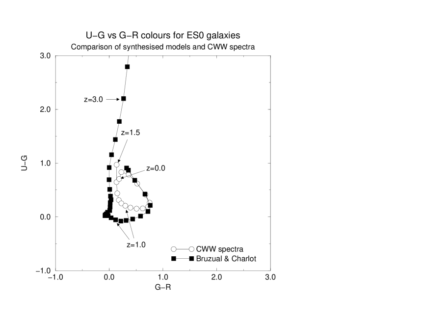
Figure 1: Comparison of U-G and G-R colours based on simulated galaxy spectra for four morphological types against the empirical galaxy spectra taken from Coleman, Wu and Weedman. The points are at intervals of 0.1 in redshift

Colours derived from both sets of galaxy spectra are shown in Figure 1. Note that all the CWW spectra are much redder in both $U-G$ and $G-R$ at $z=1.5$ than the B&C spectra. At this redshift, the star formation rate in the B&C spectra is producing considerably more flux in the UV than is seen in local galaxies, consistent with the apparent star formation history (see, eg. [Madau et al., 1998]). The result is that across the optical observing band (3000Å – 8500Å), the spectra of star–forming galaxies are close to flat spectrum for $1.2<z<2.3$. The success of the Lyman–limit imaging searches for $z\gtrsim 3$ galaxies using B&C–derived spectra indicates that at least some galaxies match these simulated spectra at high redshift.

The approach adopted by Gwyn ([Gwyn, 1998]) has changed since his 1996 paper ([Gwyn and Hartwick, 1996]) on photometric redshifts in the Hubble Deep Field (HDF). Previously, he relied on using spectra derived entirely from B&C simulations. Now, where HDF galaxies are found to be at $z\leq 1.5$ using the B&C spectra, he derives new photometric redshifts from colours based on the CWW spectra and reports improved accuracy when compared against spectroscopic redshifts. However, this results in a large hiatus between the colours of a $z=1.6$, B&C–derived galaxy and a $z=1.5$, CWW–derived galaxy, which is unsatisfactory, as can be seen in Figure 1.

To attempt to make use of the CWW spectra to more accurately estimate the colours of low–redshift galaxies, we have used the following approach:

for $z\leq 0.5$,	galaxy colours are derived only from the
	CWW empirical spectra;
for $0.5<z\leq 1.5$,	galaxy colours are interpolated smoothly between the
	two sets of models, with colours at $z\sim 0.6$ being
	closest to the CWW galaxy colours, and the colours at
	$z\sim 1.5$ being closest to the B&C colours;
for $z>1.5$,	galaxy colours are derived only from the
	B&C simulated spectra.

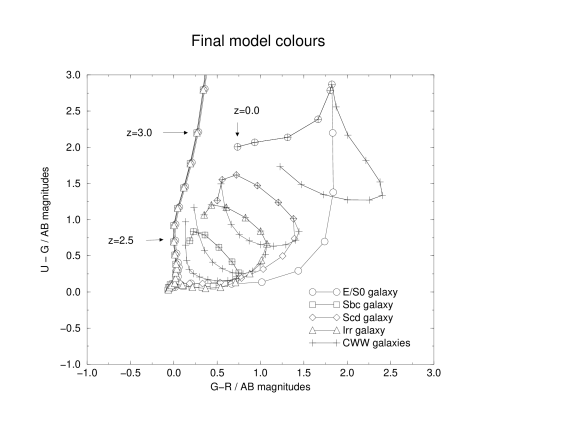
Figure 2: Final model colours. Points shown are at intervals of 0.1 in redshift.

The final galaxy models used are illustrated in Figure 2. The CWW spectra are over-plotted to show the differences between the models.

Four morphological types were used, corresponding to E/S0, Sbc, Scd and Irr, and spectra were produced at redshifts from 0.0 to 4.0 at 0.1 intervals. To cover the colour space more completely, these four models were interpolated linearly between the model types and in redshift, to create 13 models at redshift intervals of 0.025.

3 Matching the model spectra against the observations

Since the number of counts received even in a small faint aperture is large due to the plates being background limited, one can treat all errors as gaussian about the mean flux. Fluxes (unnormalised) for the model galaxies are derived from the model spectra by convolution with the telescope response for each filter, including atmospheric absorption and the effect of scattering within the telescope light path.

To compare the models against the observed fluxes, we used a $\chi^{2}$ test, with

$$\chi^{2}=\sum_{i}\Big{(}\frac{f\!_{i}-\alpha m_{i}}{\sigma_{i}}\Big{)}^{2},$$ (1)

where $f_{i}$ is the observed flux in filter $i$, $\sigma_{i}$ is the error in observed flux in filter $i$, and $m_{i}$ is the model flux in filter $i$. To obtain the optimum fit between the model and the observed fluxes, we minimised $\chi^{2}$ with respect to $\alpha$.

However, given the range of models available, it is important to determine the range of best–fit models which are consistent with the observations, and for this we used a relative likelihood method. The likelihood of obtaining an observed set of fluxes $f_{i}$ with errors $\sigma_{i}$ from model fluxes $m_{i}$ (where $m_{i}$ is a function of redshift, $z$, and morphological type, T) is

$$L(z,T)=\prod_{i}\exp\bigg{[}-\frac{1}{2}\Big{(}\frac{f\!_{i}-\alpha m_{i}(z,T)}{\sigma_{i}}\Big{)}^{2}\bigg{]}.$$ (2)

This assumes that the errors in the observed fluxes are described by a Gaussian distribution – a good assumption. From this likelihood distribution, the modal redshift can be determined by identifying the model with the highest likelihood.

Since one can apportion a probability to each model, one can use this to determine not only the most likely model, but also the mean redshift and the range of acceptable redshifts which are consistent with the observations within some relative confidence level. This is important, since for any set of models the distribution of likely models may not be mono–modal. We can use the difference between the mean and modal redshifts as a simple discriminator to identify cases where the redshift is not well constrained.

4 Redshift distribution

4.1 Overview

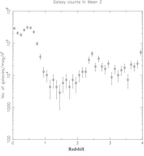
Figure 3: Distributions based on photometric redshifts for all objects with $R<26.0$

The two redshift distribution histograms, based on mean and most probable redshift, are plotted in Figure 3. The main features of both these diagrams are the two peaks: one at $0<z<0.6$, and the other at $z\approx 2.4$, with only a small number of objects lying in the range $1.0<z<2.2$. This is reinforced by studying the distributions of objects in space against redshift – these are plotted in Figure 4.

It is clear that the apparent lack of objects in this redshift range is not a real effect – there cannot really be so few objects in this region. Identifying the cause of this effect is important for understanding the limitations of the photometric redshift technique.

From the model colour tracks plotted against the actual objects colours (Figure 5), it is clear that the close–packing of the model colours in the redshift range $1.0<z<2.1$ is a problem. This arises because the continuum of the galaxy spectra is almost flat for all spectral types at wavelengths between 1400Å and 2500Å. Only the $R-I$ colours provide any redshift sensitivity for objects with $1.0<z<1.5$. The model colours effectively act as an ’attractor’ for objects with similar colours – ’attracted’ objects are labelled with the redshift and type of the model they end up with. Thus closely spaced models are less effective at distinguishing objects, unless there are significantly more objects concentrated in that area. Even then, the similarity of the objects is sufficient to make the accurate determination of the redshift impossible in this redshift range given these filters. The result is that objects with redshifts $1.0<z<2.1$ end up being pushed to lower ($z\approx 0.8$) or higher ($z\approx 2.4$) estimated redshifts.

Beyond the limitations imposed by the filter selection, it is also notable that the number of objects that are close to the models SED colours is small in the redshift range $1.0<z<2.0$. This suggests that the model colours being applied here do not directly correspond to observed colours in the field. This raises several possibilities:

1. the model colours are inaccurate;

2. there are significant systematic errors in the catalogue calibration;

3. the model colours are correct, but the observed colours differ due to reddening caused by the presence of dust in these objects.

The accuracy of a catalogue’s photometric measurements can be qualified by examining the accuracy of the photometric calibration, both as determined from the original calibrators and in comparison with other published results. All the calibrators used in the creation of the catalogue have high signal–to–noise, and even including the possibility of poor background level determination, the calibrations are at worst inaccurate by $\pm 0.05$ magnitudes in all filters. This is not sufficient to bias the results as dramatically as observed here. In comparison with other published photometric measurements for the field, such as Hu & Ridgway’s multi–filter imaging around Quasar A ([Hu and Ridgway, 1994]), the results are all consistent within the photometric errors.

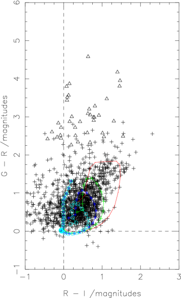
Figure 6: $G-R$ vs $R-I$ plot overlaid with the revised models colour tracks used in the determination of the photometric redshifts.

Since the model colours here are based on unreddened spectra, it seems reasonable to suggest that the lack of objects with such blue colours is due to reddening of these objects by dust. This would have the greatest effect in the $U$ & $G$ colours, since these are the ones with the shortest wavelengths. If we examine the spread of colours of the objects in $G-R$ and $R-I$ (Figure 6) we can see there is better coverage of the model tracks in $R-I$ than in $G-R$. The objects at $R-I<-0.5$ are all within 2-$\sigma$ of $R-I=0$; ie this is most probably photometric scatter. This is particularly noticeable in $R-I$ because of the lower depth of the $I$ image compared with the rest of the broadband colours.

4.2 Most likely or mean redshift?

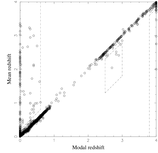
Figure 7: Most likely redshift plotted against the mean redshift

Comparing the two estimates shows several interesting features, as illustrated in Figure 7. In 1486 out of 1665 objects with $R<26.0$ , there is less than 0.1 difference between the modal and mean redshift. 63 objects differ by 0.1 – 0.2 in redshift, and 116 differ by more than 0.2. For those objects whose redshift determinations differ by greater than 0.2, these divide into three major groups: those which have a modal redshift $0<\textrm{modal~{}}z<0.6$ but have a large mean redshift, a set with $2.5<\textrm{modal~{}}z<3.0$ but a mean redshift of $1.8<\textrm{mean~{}}z<2.7$, and a set with $\textrm{modal~{}}z\approx 4.0$ but a lower mean redshift.

In Figure 8, we plot the precision of the redshift estimates as a function of $R$ magnitude. The objects which show the greatest differences are all faint ($R>24.0$); the $\chi^{2}$ fitting is looser due to the greater flux uncertainties. This in turn leads to more models sharing similar model–fitting likelihoods and a greater spread of redshifts with which the models are statistically acceptable. Examination of the precision of the redshift estimates against the modal redshift (Figure 9) shows that the majority of objects with $0<\textrm{modal~{}}z<0.8$ have small standard deviations, while the fitting is generally less constrained at higher redshifts ($z>2.0$) although the average standard deviations even at $z\approx 3$ is still $\Delta z\approx 0.1$.

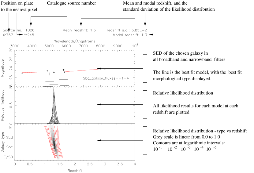
Figure 10: Explanation of the layout of the likelihood distribution graphs

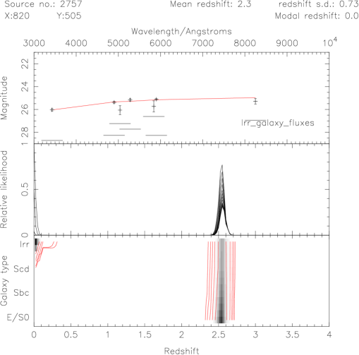
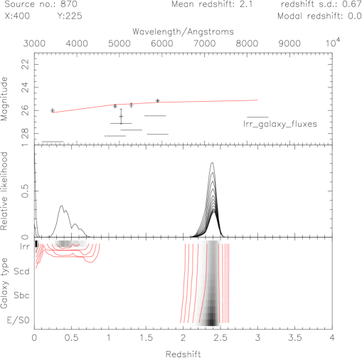
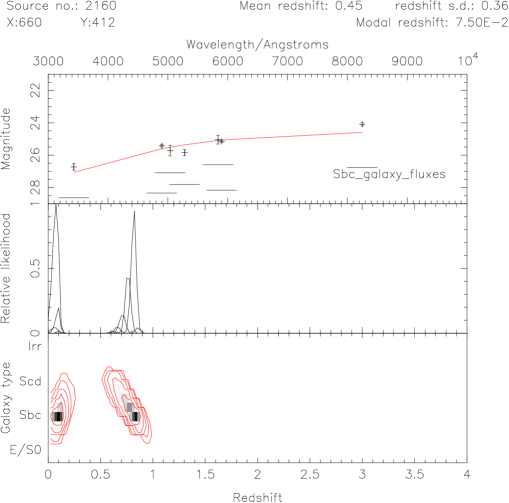
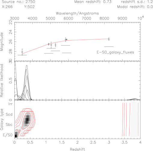
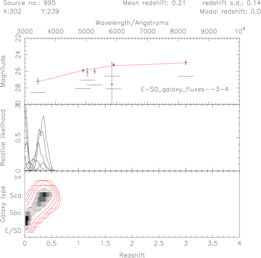
Figure 11: Examples of five objects with low modal redshifts but complex likelihood distributions

The low–redshift group ($0<\textrm{modal~{}}z<0.6$) consists of 102 objects, all of which have $24<R<26$. Some examples of the object spectra and redshift likelihood distributions are shown in Figure 11, and an explanation of the information on these graphs precedes in Figure 10

There appear to be two groups of objects which show significant differences between mean and modal redshift: faint blue galaxies which, by the nature of their flat and relatively featureless continuum, are difficult to accurately determine the redshift for without good photometric constraints; and objects with weak constraints on the $U$ magnitude which can mimic both $z\approx 0$ galaxies and spirals at $z\approx 1.0$.

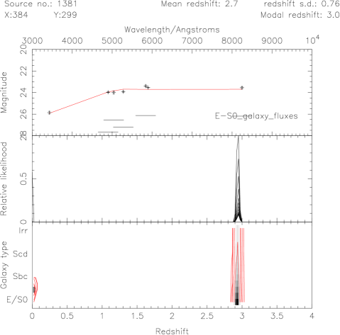
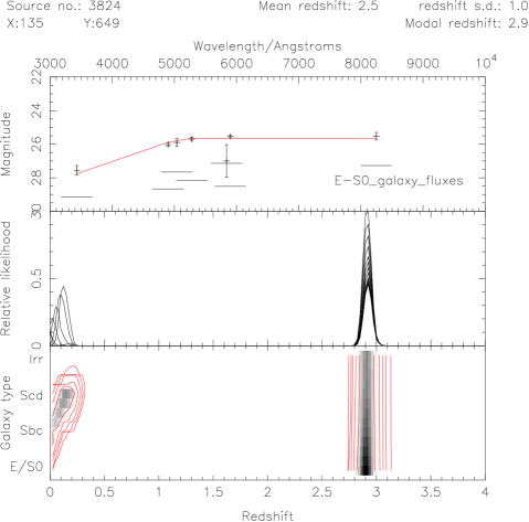
Figure 12: Two intermediate modal redshift objects with complex likelihood distributions

The intermediate ($2.5<\textrm{modal~{}}z<3.0$) and high ($3.8<\textrm{modal~{}}z<4.0$) redshift galaxies also show a fairly flat spectrum in $G$,$V$,$R$ & $I$, and red $U-G>$ colours (see Figures 12 & 13 for examples). Again this ambiguity between a low redshift E/S0/Sa galaxy with a strong 4000Å break and a high–redshift starforming galaxy with absorption due to the Ly$-\alpha$ forest and extinction below 912Å causes problems for the photometric redshift models. $J$, $H$ and other IR imaging would break this degeneracy, as would significantly deeper $U$ imaging.

In summary, the modal redshift appears to give the better redshift determination. When ambiguities arise in the determination of the redshift, the standard deviation of the redshift is sufficiently sensitive to mark the problem cases.

4.3 Low–redshift galaxies – $z<1.0$

The accuracy of the photometric redshifts is likely to be best in this sub–sample, especially in the range $0<z<0.5$. In a blind test carried out by Hogg et al, the rms deviation of the photometric redshift from the spectroscopic determination was routinely $\Delta z<0.1$, using similar methods and a similar range of wavelengths covered by the filters used here.

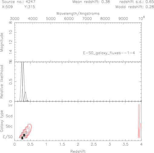
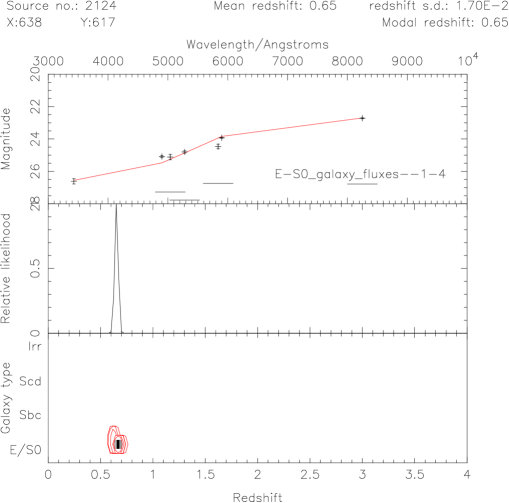
Figure 14: Two low–redshift E/S0–type galaxies

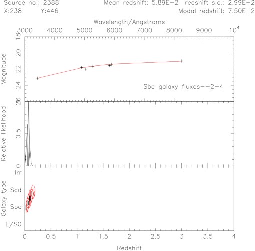
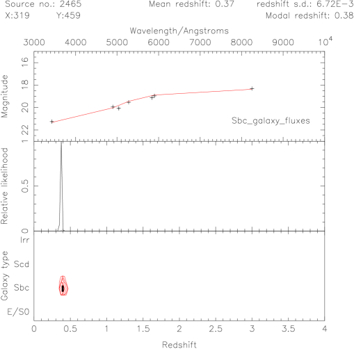
Figure 15: Two low–redshift Sbc–type galaxies

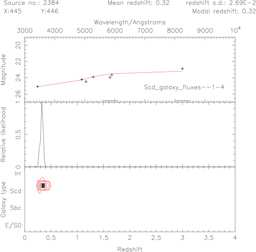
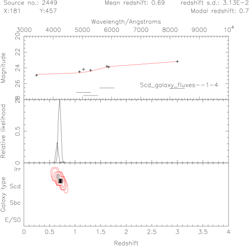
Figure 16: Two low–redshift Scd–type galaxies

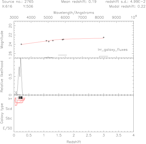
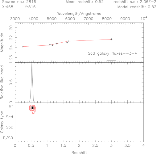
Figure 17: Two low–redshift Irr–type galaxies

Examples of redshift estimations are shown in Figures 14 – 17. These also include estimations of galaxy morphological type, made possible by the wide spread of colour space covered by the photometric models at low redshift.

A few spectroscopic redshifts for some of the galaxies in this field are already available, obtained by one of us with the WHT allowing one to check the accuracy of the photometric predictions. Table 1 shows that the photometric redshifts are accurate to $\Delta z\approx 0.15$, although the systematic offset suggests that the models can be further improved. A similar overestimate is seen in [Lanzetta et al., 1996] where the photometric models are based on redshifted CWW spectra alone, where the rms scatter was reported as $\Delta z\approx 0.15$. Comparing the published redshift for HR10 ([Graham and Dey, 1996]), it is clear that the reddening of the spectrum in this $z>1$ galaxy has resulted in an erroneous estimate.

4.4 Intermediate–redshift galaxies – $1.0<z<2.5$

As discussed in section 4.1 there are too few objects identified in the range $1.0<z<2.5$. It is important to determine what redshifts objects in this redshift range have in fact been given. Assuming that the models are at least a reasonable pointer to the correct colours, possibly affected by reddening, objects at these redshifts will have been mis-classified towards those models which have colours similar to the $1.0<z<2.1$ models. The most likely cases are therefore the low–redshift Irregular galaxies, which have relatively flat spectra in the visible wavelengths, and those models at redshifts $z\approx 0.8$ and $z\approx 2.3$ which are adjacent region we are interested in. This can actually be seen in the histogram of objects against modal redshifts (Figure 3) – there is an apparent excess of low–redshift objects at $z=0$ along with another peak in the distribution around $z=2.4$. No excess is seen at $z\approx 0.8$ but any increase here would be likely to be a small fraction of the real objects at this redshift.

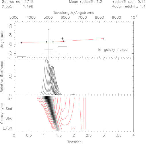
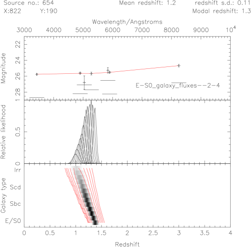
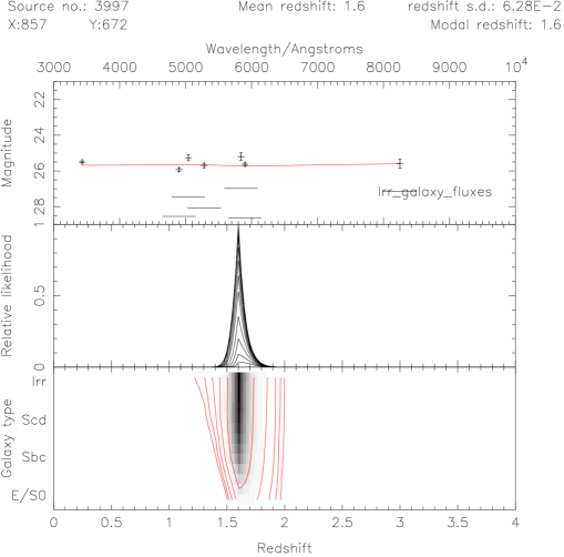
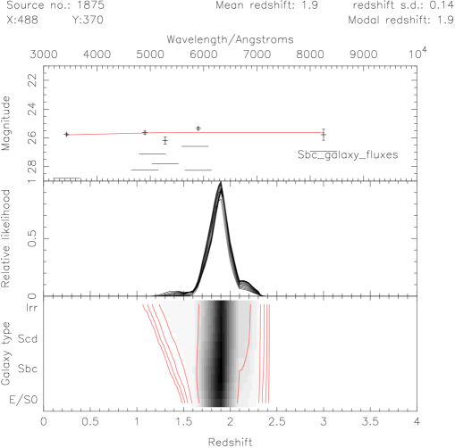
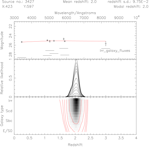
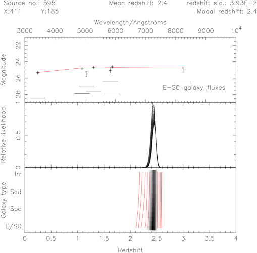
Figure 18: Six examples of galaxies with fits to model spectra $1.0<z<2.5$. Note that there is little constraint on the morphology of the objects shown here. Additionally, at $z\approx 1.3$ there is a degeneracy between morphology and redshift.

Those objects which are identified at $1.0<z<2.5$ – examples are shown in Figure 18 – are only weakly distinguished in morphological type. Additionally there is a degeneracy between morphological type and redshift estimate for galaxies with redshifts $1.0<z<1.6$ – at higher redshifts there are few major differences between the galaxy colour tracks and hence no significant discrimination between morphology based on colour evidence. To remove these degeneracies would require more IR imaging to detect the 4000Å break – this would also improve the accuracy of the redshift detections in this redshift range.

4.5 High–redshift galaxies – $2.5<z<4.0$

In Paper I, we have tried to identify galaxies at $z\approx 3$ via the 912Å break. Photometric redshifts should prove effective at determining which galaxies lie at these redshifts since they make use of all the photometric measurements together in all filters, rather than just the $U$,$G$ & $R$.

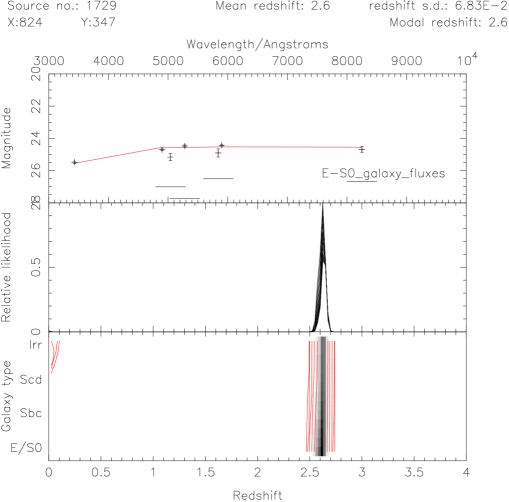
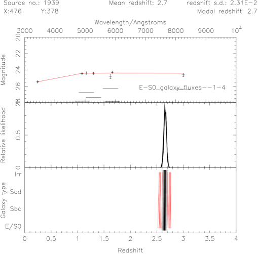
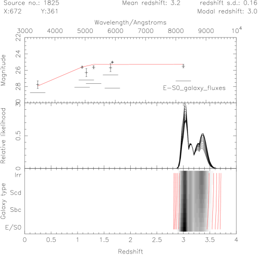
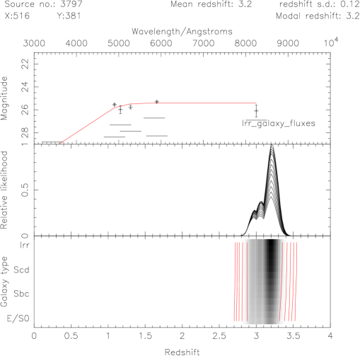
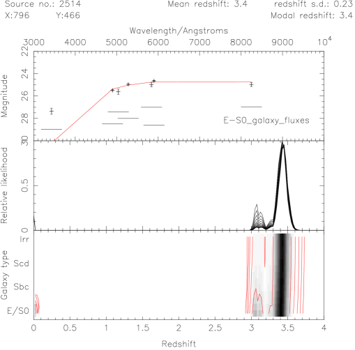
Figure 19: Examples of galaxies with fits to model spectra $z>2.5$. There is no possibility of morphological classification at these redshifts. Note that at $z\gtrsim 3.4$ the effect of the 912Å break moving into the blue end of the $G$ band starts to redden the $G-R$ colours, and that this feature is identified by the photometric redshift technique more strongly than the faint $U$ magnitudes, which have large photometric uncertainties.

Examples are shown in Figure 19. It is not possible to differentiate between different morphological types at these redshifts – the colours are too similar between the model galaxies. This is partly a result of similar star–formation histories between the model galaxies at these redshifts; this would be invalid if, for example, there were several phases of galaxy formation.

By selecting galaxies with $2.8<\textrm{modal~{}}z<3.5$, $R<25.5$ and $G>2\sigma$, we get 46 Ly–break candidates, almost twice as many as with the colour–criteria. The distribution of these galaxies (see Figure 20) also (cf Paper I) shows an apparent hole at a point mid–way between the quasars, despite the increase in surface density of candidates.

5 Clustering of objects

We can make use of the redshift determinations to look at the correlation functions for redshift subsets of the catalogue. The results of these are plotted in Figure 21.

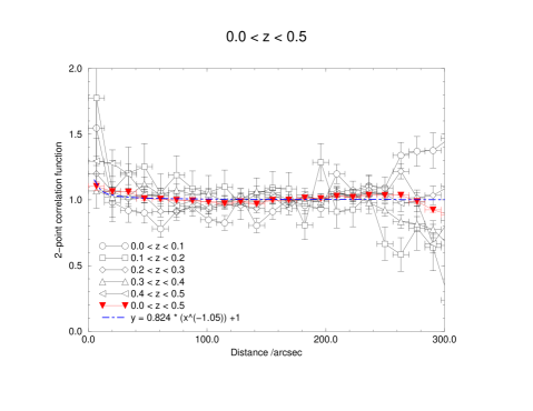
Figure 22: Correlation function for galaxies with modal redshifts $0<z<0.5$

The lowest redshift range ($0<z<0.5$) has 558 objects, and there are 352 objects in the range $0.5<z<1.0$. As a result, the statistics for these redshift ranges are sufficiently good to show that there is measurable clustering in this field at low redshifts. Fitting the standard power–law curves ($A_{\omega}\theta^{-\beta}$) to angular scales $0<\theta<150~{}\textrm{arcsec}$ gives $A_{\omega}\approx 0.82$ and $\beta\approx 1.05$ for $0.0<z<0.5$, and $A_{\omega}\approx 1.88$ and $\beta\approx 1.74$ for $0.5<z<1.0$. These are plotted in Figures 22 & 23. Also plotted in these figures are the correlation functions for subsets of the sample ordered in redshift. While the noise in these subsets is worse and no strong conclusions can be drawn, the apparent clustering of the $0.7<z<0.9$ objects at small angular scales is interesting.

In the rest of the $z$ bins there is little significant signal, with the least insignificant being 1.5-$\sigma$ clustering at $240^{\prime\prime}$ in $2.0<z<2.5$. Necessarily, there is no coverage of $1.0<z<2.0$.

6 Artificial clusters

We now test the ability of this sort of analysis to recover real features from the field. We use these redshift colour models to place a realistic spatial distribution of artificial galaxies into the images and examine the likelihood of detecting a cluster towards PC1643+4631 A&B using colour methods. We can find no similar experiment in the published literature on any field.

6.1 Theoretical magnitude and spatial distributions

To mimic a cluster of galaxies, one needs distributions for both the magnitudes and positions of the galaxies on the sky. For the former we assummed a Schechter luminosity function ([Schechter, 1976]), while for the latter we assumed a Hubble distribution, where the surface density is described by $\sigma_{0}/(1+(R/R_{c})^{2})$ ([Wu and Hammer, 1993]). We used a core radius, $R_{c}=200$kpc for the spatial distribution (Jones et al., 1997, found, for PC1643, a core radius of $\sim 300$kpc), and used half–light radii of 10kpc for the galaxies.

To determine the magnitudes of galaxies in a cluster at some redshift, we used the results from the Canada France Redshift Survey (CFRS) ([Lilly et al., 1995]), because it is one of the best measured in a constant rest frame waveband and it provides us with the best–fit $B$–band Schechter luminosity function for $z\gtrsim 0.5$ galaxies ([Lilly et al., 1995]). The CFRS contains many objects at redshifts out to $z\approx 1.1$, and provides the best estimate of the luminosity at $z\approx 0.5$. Additionally, for $z<0.9$, the $B$–band is redshifted to wavelengths covered by the $U$,$G$,$V$,$R$ and $I$ filters. Taking the values $\alpha=1.03$, absolute magnitude $M^{*}_{AB}(B)=-21.04$, we determine the observed total magnitudes from these galaxies using (see [Lilly et al., 1995])

$$I_{\textrm{AB}}=M_{\textrm{AB}}+5\log(D_{L}/10pc)-2.5\log(1+z)-(B-I_{z}),$$ (3)

$D_{L}$ is the luminosity distance, $I_{z}$ is the $I$ band shifted to shorter wavelengths by a factor of $(1+z)$, and $B$ is the magnitude in the rest–frame $B$ band. The value of $(B-I_{z})$ is taken from the photometric SED models, and hence the value of $B$ must be calculated by interpolation between the $U$, $G$ and other broadband filters. From this, observed magnitudes can be calculated for the redshift range $0<z<1.5$. For $z>1.5$, $B$ moves to longer wavelengths than $I$. A simple extrapolation of the $R-I$ colour can be used to obtain a first–order estimate of the rest frame $B$ band magnitude. This should prove to be a reasonable approximation of the real value given that the 4000Å break is weak in galaxies which are strongly star–forming, which is the case for the SED models used at $z>1$.

We do not attempt to model the evolution of the luminosity function. While this is a shortcoming of this method, at $z<0.9$, the maximum likely error is $\pm 0.5$ mag (see [Lilly et al., 1995]). Beyond $z\approx 1$, the evolution of the luminosity function is poorly constrained, but it is reassuring that the luminosity function of $z\approx 3$ galaxies have a luminosity function best fitted by $M_{*}\approx-21$ ([Dickinson, 1997]).

At low redshifts, there are significant colour differences between different morphological galaxy types, with spirals having much bluer colours than ellipticals. While the ratio of ellipticals to spiral galaxies in general is about 60:40, in the cluster environment the proportion of elliptical galaxies is often much lower, closer to 40:60 (E+S0:S+Irr) ([Dressler et al., 1997]). To simulate this spread of colours, we opted to create frames with just one morphological type in each. To keep the processing as simple as possible two plates were made, with one having E/S0 type galaxies and the other Scd/Irr types.

6.2 Method

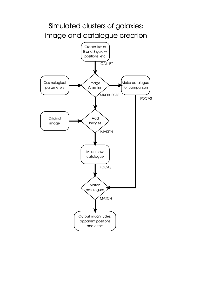
Figure 24: Flow diagram showing the procedures used for simulating images of clusters of galaxies and obtaining a catalogue from those images

The processes required to simulate each cluster at each redshift and make photometric measurements of the simulated cluster galaxies after superimposition onto the PC1643 are illustrated in Figure 24. Simulated clusters were made at redshifts from 0.1 to 4.0 in steps of 0.1.

We used the ARTGAL package in IRAF to create artificial clusters of galaxies with the required properties. For each ‘cluster’ only two images were made, one each for elliptical and spiral galaxies, made to have the same zero point and exposure time as the $I$ image, and zero background level. No additional noise was simulated because the real images are all background limited.

Recent publications discussing the distributions of the different morphological types suggest that there is some segregation, with steeper velocity dispersions for later–type galaxies (see, eg [Adami et al., 1998]). We have not attempted to mimic these results here, since our aim is to examine the ability of the tests previously carried out on this field to recover cluster members, rather than to produce a completely accurate cluster distribution.

Having generated the $I$–band spiral image at each redshift, we used the Sbc model SEDs to determine the colours of the simulated spirals in $R$,$V$,$G$ & $U$, and IMARITH was used to scale the $I$ image to mimic the correct colours in the other broadband images. We used a similar procedure to produce $R$,$V$,$G$ & $U$ images from the $I$–band elliptical image using the E/S0 model SEDs. These $I$, $R$, $V$, $G$ & $U$ spiral and elliptical images were summed together to create composite images, and a catalogue was made from the $R$ composite image using FOCAS, which we will refer to as the matching composite catalogue (MCC).

These composite images were then added onto the real PC1643 images. The resulting $R$ image was processed using FOCAS to produce a catalogue based on $R$ isophotal apertures: catalogues were then made in $I$, $V$, $G$ & $U$ using the $R$ isophotes and the five resulting catalogues were then matched using MATCH against the MCC. To extract the simulated galaxies from these newly created FOCAS catalogues, ‘stripped’ catalogues were made including objects only if they corresponded to the positions indicated by the MCC - ie these catalogues should contain only the information on the measureable simulated cluster galaxy members. These stripped catalogues were then given the same photometric redshift analysis as the real objects in the PC1643 field.

6.3 Results

Full–colour images showing the artificial cluster at various redshifts are shown in Figures 25 & 26, both in isolation and superimposed on the PC1643 field. While it is easy to recognise the cluster on its own, it becomes impossible to differentiate the cluster against the other objects in the field at $z>1.0$, and the contrast is poor even at $z=0.6$.

More importantly, it is the ability of the catalogue creation and analysis software to detect a cluster which is of greatest interest here, particularly at faint magnitudes $R\gtrsim 24$. We have plotted the $U-G$ vs $G-R$ colours for each of the simulation images illustrated in Figures 25 & 26. Even at $z=0.2$ the fainter members of the simulated galaxies show significant photometric scatter away from the expected colours, and this is reflected in the estimates of modal redshift: there is a peak at $z=0.2$ as expected, but over a third of the sample are more than 0.1 away from this redshift, and 9 of the simulated galaxies are mistaken for high–redshift galaxies at $z\gtrsim 3$.

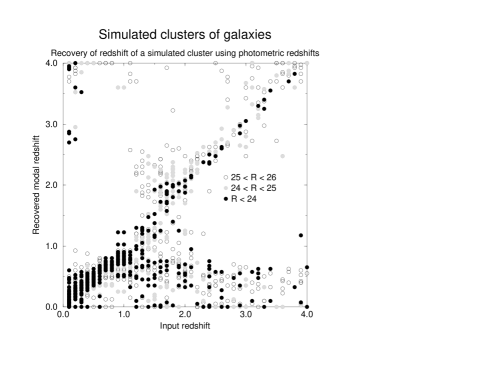
Figure 29: Modal redshift estimates based on photometry from recovering the member galaxies of simulated clusters at $z=0.1$ to $z=4.0$ in steps of 0.1 in $z$ using FOCAS. Modal redshifts are shown for all simulated galaxies which have a measured $R<26.0$.

At $z\lesssim 1.0$, the photometric–redshift technique still produces redshift estimates around the expected value, with increased scatter as the simulated cluster becomes fainter with increasing redshift (see Figures 29 & 30). This is also reflected in the increased scatter of the $U-G$ and $G-R$ colours, which, it should be stressed, is often greater than 3-$\sigma$, where $\sigma$ is the photometric error based on the noise for the object. This is the result of pollution of the isophotal apertures by nearby neighbours, which is inevitable in a deep, ground–based field like this one. Given that the density of objects in the field including all detections down to the surface brightness limits of 3-$\sigma$ in an area of six pixels is approximately one object in every $5^{\prime\prime}\times 5^{\prime\prime}$ box, and that the average isophotal area of a object with $R=25.0$ is some 5 arcmin², this means that at least one in five faint objects will overlap another faint object, so that in this set of deep images, objects are being confused.

To determine whether a significantly brighter cluster of galaxies would be visible in this field, we repeated the simulation with all the magnitudes brightened by one magnitude. Bearing in mind that this is the most extreme error likely in the simulation, this is also a good test of the sensitivity of these simulations to the real magnitude distribution. Even with many more members, such a cluster would still be difficult to distinguish using colour–criteria or by excess surface density.

At intermediate redshifts, $1.0<z<2.0$, the photometric redshift technique fails to correctly determine the redshift in almost all cases. Despite starting from simulated galaxies with the correct colours, the colours of the galaxies as recovered from the field are systematically scattered to redder colours. There may be a systematic effect resulting from selecting objects based on their $R$ magnitudes — for example, objects which are polluted to fainter magnitudes in $R$ are missed from the sample, whereas objects which recover fainter $G$ magnitudes than originally simulated appear redder than they really are. There may also be a systematic effect from the different surface densities of objects in $R$ and $G$ at similar magnitudes – there are 763 objects with $25<R<26$, and only 537 with $25<G<26$ – so objects with $G-R\approx 0$ stand proportionally more chance of being brightened in $R$ than in $G$. Additionally, if the position of a simulated galaxy does coincide with that of a real object, it is likely that the real object has $G-R\gtrsim 0.5$, and hence the pollution of the simulated object will result in redder measured colours.

This failure to accurately detect galaxies in the range $1.0<z<2.0$ is a function of the filters used. Because there are no strong continuum features over the wavelengths spanned by the optical filters used here at these redshifts (approximately 1200Å – 4000Å) the photometric redshift are poorly determined. Additionally, because of the scatter of the objects colours away from the simulated colours, objects with redshifts in the range $1.0<z<2.0$ are scattered to lower and higher redshifts. This is clearly seen in Figures 29 & 30. The result is that any histogram of galaxies over the redshifts estimated from photometric techniques using a similar range of filters to those used here will show a deficit of galaxies with $1.0<z<2.0$ and peaks above and below this range against the true population of galaxies. Precisely this behaviour is seen in the redshift distribution calculated from the HDF four–colour photometry (in F300W, F450W, F606W and F814W) using photometric redshifts (see [Gwyn and Hartwick, 1996] and to a lesser extent [Sawicki et al., 1997]). The deficit is not quite so marked as it is in the photometric redshifts estimates of the field of PC1643, due to slight differences in modelling but the effect is still the same. It is notable that the photometric redshift estimates of [Lanzetta et al., 1996] (LYFS) do not suffer from this effect, and appear to produce a smooth redshift histogram: the photometric models used by LYFS are based entirely on the CWW spectra extended into the UV without including the effects of evolution, with the effects of the $\textrm{Ly--}\alpha$ forest and 912Å break taken into account. However, the galaxies at $z\approx 3$ are predicted to have $U_{300}-V_{450}\approx 5$ and $V_{450}-R{606}\approx 1.0$ by LYFS, which is considerably redder in $U_{300}$ than those detected by [Steidel et al., 1996a] which have $U_{300}-V_{450}\approx 2$ and $V_{450}-R_{606}\approx 0.5$, and therefore casts doubt onto their photometric models.

To test just how much brighter a distant cluster would have to be to be clearly evident, we increased the magnitudes of every member of the simulated cluster at $z=2.0$ until the cluster just became evident in the images. We emphasize that significantly more than two magnitudes of brightening would be required to make the cluster stand out from the field. We stressed that this is far more than the largest expected error in the brightness of these simulations.

At $z\gtrsim 2.3$, the 912Å break starts to extinguish a $U$–band observation, and by $z\approx 3$ provides a clear colour signature, ie $U-G>2.0$. This feature has been successfully used to detect high–redshift galaxies both with custom filters and in the HDF (eg [Steidel and Hamilton, 1993], [Steidel et al., 1996a]). Most of the galaxies previously detected at $z\approx 3$ have $R\gtrsim 24.5$ [Steidel et al., 1996b], which is consistent with the brightest members of the simulated cluster at the same redshift (Figure 31). Intriguingly, while the photometric redshift estimations do peak at around their expected value, there is also a significant proportion which are mistaken for low–redshift galaxies (again, see Figures 29 & 30). From the 123 simulated galaxies with colours consistent with $2.5<z<3.0$ and measured $R<26.0$, 52 are identified as having $z>2.5$ and 70 are identified as low redshift galaxies with $z<0.8$. If this mimics the real situation for detecting $z\approx 3.0$ galaxies, then it suggests that a significant number of high–redshift galaxies are missed if redshifts are estimated using photometric techniques. Note also that the limiting magnitudes of [Steidel and Hamilton, 1993] etc. are similar to those of the PC1643 images.

To investigate the efficiency of selecting $z\approx 3$ galaxies using the colour–criteria described in Paper I, we concatenated the simulated catalogues with $2.5<z<3.5$ and selected objects with $R<25.5$ and $G>2\sigma$. While the simulations were carried out to mimic a cluster of galaxies, there is negligible overlap between the individual simulated galaxies in each catalogue. Therefore, while there is clustering of the galaxies in the field, it is important to note that the photometric spread and the results are similar to that which would be obtained for a random uniform spatial distribution.

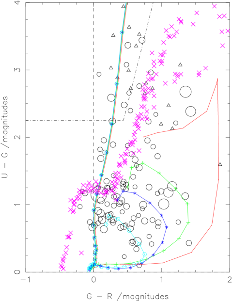
Figure 32: $U-G$ vs $G-R$ colour–colour graph for simulated galaxies with $2.5<z<3.5$. All objects shown have measured $R<25.5$ and $G>2$–$\sigma$. The triangles denote 1–$\sigma$ lower limits in $U-G$. The cross are stars taken from the Gunn & Stryker database, and the dot–dash line is the bound for selecting high redshift candidates. The tracks plotted on this graph are the model colours for galaxies at various redshifts: the point at $U-G=2.2$ and $G-R=0.3$ is at $z=3.0$, and points at larger $U-G$ are at higher redshift in steps of $\Delta z=0.1$.

Figure 32 shows the measured $U-G$ vs $G-R$ colours of these 104 objects. We note that the simulated objects are scattered from the simulated colours to such an extent that only 12 of the objects show measured $U-G$ and $G-R$ colours consistent with objects at $z\approx 3$. Of these same 104 objects, 48 are identified as being at $z>2$ by the photometric redshift estimator (see Figure 33). Even if we take just the catalogue for the simulated cluster at $z=3.0$, of the 12 objects with $R<25.5$ and $G>2\sigma$, only two meet the colour–criteria, whereas eight are identified as having estimated $z>2$. Therefore, five–colour photometric redshifts appear to provide a more effective method of detecting high–redshift galaxies than the three–colour $UGR$ method used by Steidel et al. This is not surprising since the extra photometric measurements provide extra constraints, which reduce the effects of individual photometric measurement errors.

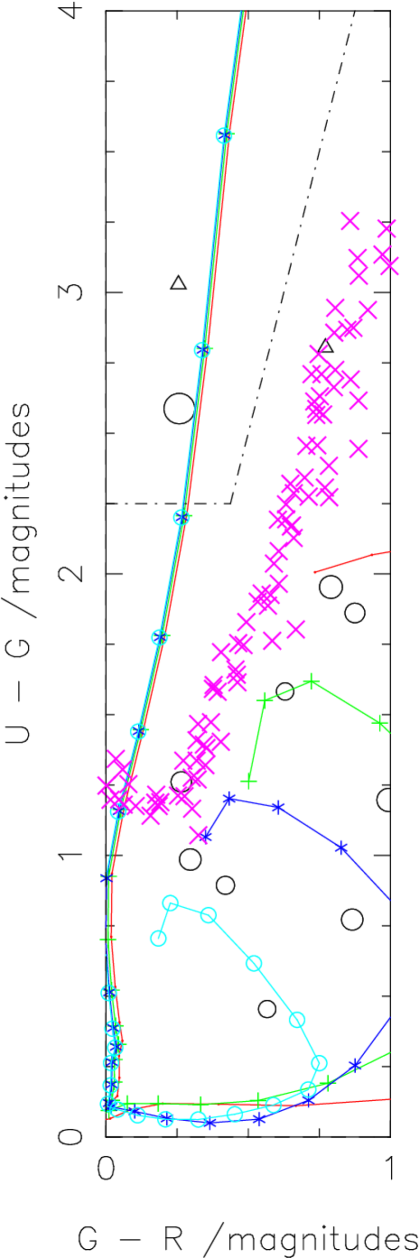
Figure 34: Comparison of the $U-G$ vs $G-R$ colours between simulations with galaxies with angular sizes $\approx 10$kpc (left) and galaxies with angular sizes of $\approx 2.5$kpc (right). The dashed line denotes the limit of the colour–criteria used to select Ly–break galaxies. All objects plotted have $R<25.5$ and $G>2\sigma$: circles represent $>1\sigma$ detections in $U$,$G$ and $R$; triangles denote 1–$\sigma$ lower limits for $U-G$.

Comparing the angular sizes of the simulated objects against Ly-break galaxies observed in the Hubble Deep Field suggests that these galaxies should be about 2–3kpc in size ([Dickinson, 1997]), which is considerably smaller than the sizes used in this simulation, which are $\approx 10$kpc in size. We repeated the $z=3.0$ simulation to assess whether the angular sizes used had a significant effect, with the angular sizes of the simulated galaxies reduced by a factor of four. This small angular size simulation had 15 objects with $R<25.5$ and $G>2\sigma$, of which three fulfilled the colour–criteria, whereas using photometric redshifts, 8 were identified at $z>2$. Figure 34 compares the $U-G$ vs $G-R$ colours for the original and revised simulation.

The increase in numbers of galaxies detected is due to the increase in the peak flux of galaxies due to smaller half–light radii – this makes it easier for FOCAS to detect these galaxies as their peak fluxes are more likely to be greater than the $3\sigma$ detection threshold. It is important to note that decreasing the angular size of the simulated galaxies has not had a significant effect on the fraction of galaxies which fulfill the colour criteria for $z\approx 3$ galaxies: one might expect reducing the angular size to reduce the level of confusion observed in these simulations; however, while the peak flux increases and the area covered by the object is decreased for all objects, this also promotes simulated objects which were previously too faint to be detected above the detection threshold and it is these faint objects which are most likely to be significantly affected by confusion with the many real faint objects in the field. The effect of confusion on objects with faint (ie $R>24$) magnitudes is to “average” the simulated object’s colours with that of the confusing object, with the result that a large proportion of the sample is moved towards the average colours of the real objects in the field, ie $U-G\approx 1.2$ and $G-R\approx 1$.

From these results, it appears that the colour–criteria of [Steidel et al., 1995] is missing a large fraction, 5 out of 6, of the real population of $z\approx 3$ galaxies. This is the result of confusion due to the $\approx 1^{\prime\prime}$ seeing in the images; one would therefore expect to find considerably greater numbers of Ly–break galaxies in the HDF. There are 26 galaxies in the HDF which have spectroscopic redshifts $z>2$ ([Dickinson, 1997]), of which 12 have $2.8<z<3.5$ and $V_{606}<25.5$ (this is consistent with the spectroscopic redshifts of Ly–break candidates; see [Steidel et al., 1996b] and the faint magnitude limit). The area of the Hubble Deep Field is 4.5 arcmin² and one would expect, given the published surface–density of “robust” Ly–break candidates of $\approx 0.7$ arcmin^-2 ([Steidel et al., 1998]) to find only 3 Ly–break candidates in the HDF. Because the HDF covers such a small field of view, there may be significant differences in the numbers of Ly–break galaxies between adjacent fields, but it is striking that the factor of apparent overdensity of Ly-break galaxies seen in the HDF is equivalent to the factor of Ly-break galaxies lost to confusion in the ground–based images.

In [Dickinson, 1997], the luminosity function of $z\approx 3$ galaxies is illustrated, but the HDF count of $z\approx 3$ galaxies have been renormalised to the numbers seen in the ground–based images. We suggest that the surface density seen in the HDF is a better estimate of the real surface density of $z\approx 3$ galaxies, and there are approximately 6 times more $z\approx 3$ galaxies than currently thought. This has important consequences for the understanding of the star–formation history of the universe and would suggest that the peak rate of star–formation occurred at an earlier epoch than currently thought (see [Madau et al., 1998]).

To definitively identify the majority of Ly–break candidates and determine the real surface–density of these galaxies, observations with much improved seeing will be necessary; either by further HST observations to increase the area of sky observed and thereby reduce the effects of cosmic variance, or by deep ground–based observations with adaptic optics to reduce the point–spread–function in the images. The effects of confusion can be quantified using similar simulations to those demonstrated here.

7 Conclusions

In using the multicolour photometric redshift technique on the objects found in the deep imaging of PC1643+4631, we have shown the following.

1. The technique is efficient at identifying objects at $z\lesssim 1$ where the photometric errors are small, ie at $R\lesssim 24$, because the $\chi^{2}$ fitting is well constrained because the colours change strongly with redshift.

2. These photometric redshifts are in broad agreement ($\Delta z\approx 0.15$) with the 4 spectroscopic redshifts in the range $0.62<z<0.81$ in the PC1643+4631 field, whereas HR10 at $z=1.44$ has a colour–estimated redshift of $z=0.65$, indicating that either significant reddening can distort the redshift determination or that at $1<z<2$ the photometric technique fails.

3. Ground–based morphological classification is possible on low–redshift ($z\lesssim 0.7$) objects with high signal–to–noise photometry (ie $R<24$ in the deep PC1643 images), although this work does not investigate its accuracy, due to the difficulties in obtaining secure morphological classifications for a significant number of galaxies in this field by manual or automatic means.

4. There are degeneracies between the morphological type and redshift in objects with $1.0\lesssim z\lesssim 1.6$, due to the models with different morphologies having similar colours at differing redshifts.

5. No constraints can be placed on the morphology of high redshift ($z\gtrsim 3$) galaxies using these models since there is no significant difference between the colours of the model galaxies with different morphologies at $z\gtrsim 2$.

6. 46 Ly-break candidates have been identified in the PC1643 images with $2.8<z<3.5$, $R<25.5$ and detected at $>2\sigma$ in $G$; the distribution of these candidates still shows an underdensity mid–way between the quasars.

7. The histogram of photometric redshift estimates shows two peaks, at $z\approx 0.7$ and $z\approx 2.3$, and few objects with $1.0<z<2.0$. This is probably an artifact of the photometric redshift technique, arising from the close–spacing of the model colours at these redshifts, and the histogram is therefore not indicative of the real distribution of redshifts.

8. By calculating both modal and mean photometric redshifts, as well as a standard deviation for the likelihood distribution, for each object, ambiguous photometric redshift estimates can easily be flagged using $|\textrm{modal }z-\textrm{mean }z|>0.2$, giving an advantage over previous modal–only methods.

9. There is evidence of clustering in the field at low ($z\lesssim 0.9$) redshift which is consistent with other published results.

We have carried out simulations to examine the ability of the photometric redshift technique to accurately recover simulated galaxies at various redshifts. These show the following.

1. For simulated galaxies at $0.1<z<0.3$, faint E/S0 galaxies are mistakenly identified as $z\gtrsim 3$ galaxies because of the red $U-G$ colours. An E/S0 with $R\approx 24$ will often have no detected flux in $U$, and be mistaken for a Ly–break candidate.

2. For simulated galaxies at $0.1<z<1.0$, the average estimate of redshift is consistent with the simulated redshift, but there is a spread of $\Delta z\approx 0.2$ in the distribution. This is partly due to the photometric errors causing the colours of the object to move away from the simulated colours, but also due to contamination of the object colours by other objects in the field.

3. For simulated galaxies at $1.0<z<2$, the photometric redshift is unreliable and misclassifies these galaxies to lower ($z\approx 0.6$) and higher ($z\approx 2.2$) redshifts, resulting in peaks in the photometric redshift distribution which are not representative of the real redshift distribution. This is a fundamental problem with photometric redshift estimates based only on optical imaging. A similar problem is seen in several publications in the literature but has not been appreciated (see [Gwyn and Hartwick, 1996] and [Sawicki et al., 1997], who both have a decrease in numbers of galaxies between $1<z<2$ but considered it a real observation), which has resulted in erroneous conclusions being drawn.

4. For simulated galaxies at $z>2.5$, the photometric technique is effective in detecting about half the sample as being at $z>2.5$, with the rest of the sample being mistaken for low redshift galaxies.

5. Photometric estimates may prove effective in selecting high redshift galaxies at $z\approx 3$, where the $U-G>2$ colours and fairly flat spectrum in $G$,$V$,$R$ and $I$ provide additional constraints to the three colour $U$,$G$,$R$ method currently used for successfully selecting $z\approx 3$ galaxies.

6. The scatter of the simulated galaxies away from their simulated colours is two to three times greater than that expected from the photometric errors alone and arises as a result of confusion between the simulated galaxies and the real objects in the field. Since the amount of confusion is directly related to the resolution of the images, the WHT images will be far more affected by confusion than equivalently deep HST images.

7. Because of the effects of confusion, the current published estimates of the surface densities of Ly–break galaxies based on ground–based imaging are under–estimates by a factor of $\approx 6$; such an increase in the surface density of these galaxies is consistent with the surface densities seen in the HDF.

8. Any third image of a single quasar causing the PC1643 pair is extremely likely to be confused and therefore unrecognisable.

9. Deep ground–based CCD imaging without adaptive optics is inevitably confusion–limited at $R>26.0$. Imaging with smaller point–spread–functions is the only way to alleviate this.

Simulations have been carried out to investigate the difficulties in identifying a cluster at various redshifts in the PC1643 field. These show the following.

1. Even with our many optical colours, it is difficult to visually identify a cluster of galaxies at $z\approx 0.4$ against the other objects in any deep field. A cluster at $z=1$ with galaxy luminosities similar to those seen locally would be lost against the other objects in the field.

2. Even a very rich cluster at $z\approx 1.0$ would be impossible to distinguish from the field on the basis of this $U$, $G$, $V$, $R$ and $I$ imaging and hence the evident absence of a cluster in these $1.1^{\prime\prime}$ resolution images is entirely consistent with a distant cluster producing the CMB decrement seen.

3. A cluster at $z=1.0$ in which each member was 1 magnitude brighter than expected would still be difficult to detect; however, if the members were more than 2 magnitudes brighter, the cluster would be evident in the images.

8 Acknowledgements

GC acknowledges a PPARC Postdoctoral Research Fellowship. TH acknowledges a PPARC studentship. We thank Steve Rawlings for obtaining the redshift of galaxy 4 in Table 1.

	Spectroscopic	Photometric
Object	redshift	redshift
1	$0.659\pm 0.002$	$0.55\pm 0.03$
2	$0.670\pm 0.002$	$0.57\pm 0.04$
3	$0.670\pm 0.002$	$0.52\pm 0.05$
4	$0.810\pm 0.003$	$0.62\pm 0.08$
HR10	$1.44\pm 0.01$	$0.65\pm 0.08$

Table 1: Comparison of spectroscopic and photometric redshifts in PC1643

Figure 4: Angular distributions versus redshift for all objects with $R<26.0$. EW position is the offset from the centre of the field along the X–axis of the CCD. NS position is the offset form the centre of the position along the Y-axis of the CCD.

Figure 5: U-G vs G-R plot overlaid with the revised models colour tracks used in the determination of the photometric redshifts.

Figure 8: Standard deviations of the redshift distributions for each object plotted against $R$ magnitude.

Figure 9: Standard deviations of the redshift distributions for each object plotted against modal redshift.

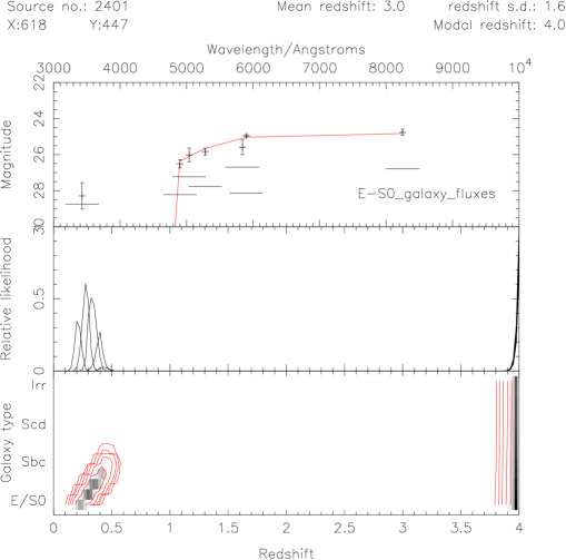
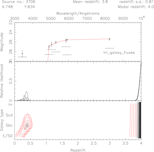
Figure 13: Two high modal redshift objects with complex likelihood distributions

Figure 20: The distribution of the Ly–break candidates, which are marked as circles, selected using $R<25.5$, $G>2\sigma$ and $2.8<\textrm{modal~{}}z<3.5$.

Figure 21: Comparison of the clustering of the galaxies in the field in different redshift ranges

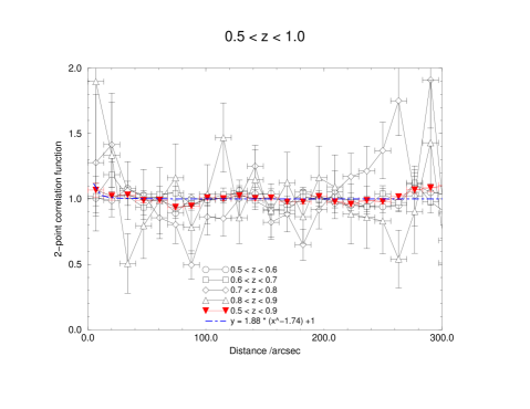
Figure 23: Correlation function for galaxies with modal redshifts $0.5<z<1.0$

This figure is avaliable at ftp.mrao.cam.ac.uk:/pub/PC1643/paper2.figure50.eps

Figure 25: Colour images of the simulated cluster at $z=0.4$, $z=0.6$ and $z=0.8$. Images on the left are on a blank background; those on the right are superimposed on the PC1643 field. All these images use the same colouring scheme used in Cotter et al., 1998.

This figure is avaliable at ftp.mrao.cam.ac.uk:/pub/PC1643/paper2.figure51.eps

Figure 26: Colour images of the simulated cluster at $z=1.0$, $z=2.0$ and $z=4.0$. Images on the left are on a blank background; those on the right are superimposed on the PC1643 field. All these images use the same colouring scheme used in Cotter et al., 1998.

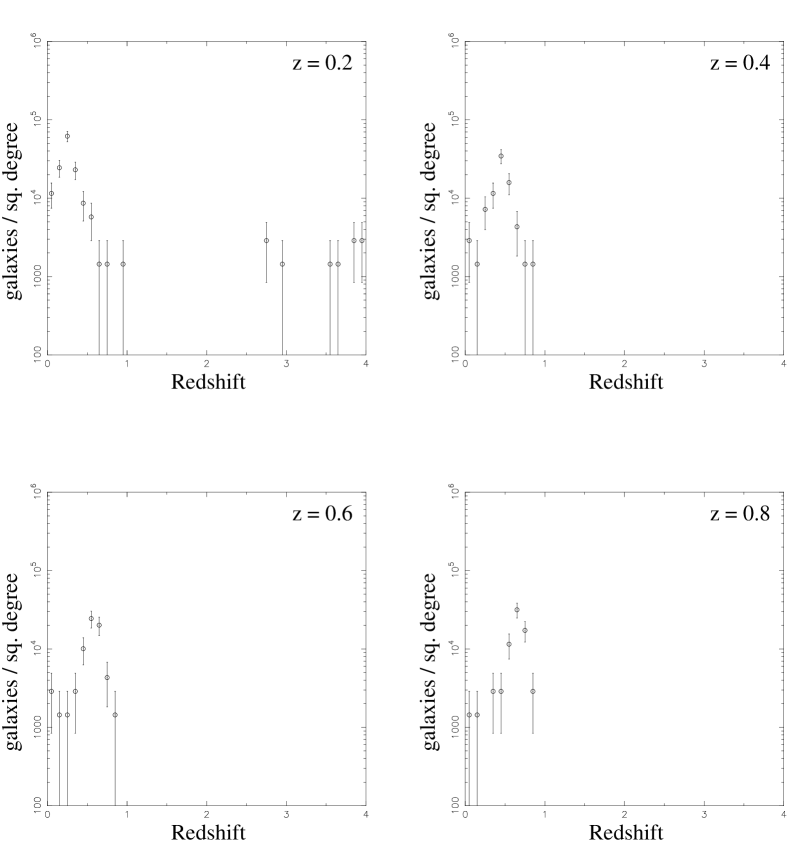
Figure 27: The histogram of modal redshifts as estimated from photometric measurements of the simulated galaxies. These graphs illustrate the effect of attempting to recover the simulated galaxies from the PC1643 field using FOCAS at $z=0.2$, $z=0.4$, $z=0.6$ and $z=0.8$. Only simulated galaxies with measured $R<26.0$ are shown.

Figure 28: The histogram of modal redshifts as estimated from photometric measurements of the simulated galaxies. These graphs illustrate the effect of attempting to recover the simulated galaxies from the PC1643 field using FOCAS at $z=1.0$, $z=2.0$, $z=3.0$ and $z=4.0$. Only simulated galaxies with measured $R<26.0$ are shown.

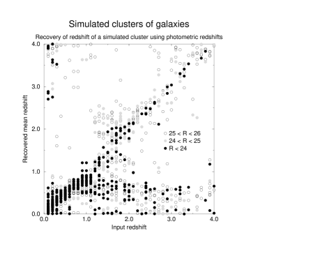
Figure 30: Mean redshift estimates based on photometry from recovering the member galaxies of simulated clusters at $z=0.1$ to $z=4.0$ in steps of 0.1 in $z$ using FOCAS. Mean redshifts are shown for all simulated galaxies which have a measured $R<26.0$.

Figure 31: $R$ magnitude distribution for the simulated cluster at $z=3.0$

Figure 33: Histogram of the photometric redshift distribution measured from a simulated catalogue containing objects with simulated colours consistent with galaxies at $2.5<z<3.5$.

References

- [Adami et al., 1998] Adami, C., Biviano, A., and Mazure, A. (1998). Segregations in clusters of galaxies. A&A, 331:439–450.
- [Bruzual and Charlot, 1993] Bruzual, G. A. and Charlot, S. (1993). Spectral evolution of stellar populations using isochrone synthesis. ApJ, 405:538–553.
- [Coleman et al., 1980] Coleman, G. D., Wu, C. C., and Weedman, D. W. (1980). Colors and magnitudes predicted for high redshift galaxies. ApJS, 43:393–416.
- [Dickinson, 1997] Dickinson, M. (1997). Color-Selected High Redshift Galaxies and the HDF. In Livio, M. Fall, S. and Madau, P., editors, The Hubble Deep Field, STScI Symposium.
- [Dressler et al., 1997] Dressler, A., Oemler, Augustus, J., Couch, W. J., Smail, I., Ellis, R. S., Barger, A., Butcher, H., Poggianti, B. M., and Sharples, R. M. (1997). Evolution since z = 0.5 of the Morphology-Density Relation for Clusters of Galaxies. ApJ, 490:577+.
- [Graham and Dey, 1996] Graham, J. R. and Dey, A. (1996). The redshift of an Extremely Red Object and the nature of the very red galaxy population. ApJ, 471:720+.
- [Gwyn, 1998] Gwyn, S. D. J. (1998). Photometric redshifts. World Wide Web page, University of Victoria, Canada. http://astrowww.phys.uvic.ca/grads/gwyn/pz/index.html.
- [Gwyn and Hartwick, 1996] Gwyn, S. D. J. and Hartwick, F. D. A. (1996). The redshift distribution and luminosity functions of galaxies in the Hubble Deep Field. ApJ, 468:L77–+.
- [Hogg et al., 1998] Hogg, D. W., Cohen, J. G., Blandford, R., Gwyn, S. D. J., Hartwick, F. D. A., Mobasher, B., Mazzei, P., Sawicki, M., Lin, H., Yee, H. K. C., Connolly, A. J., Brunner, R. J., Csabai, I., Dickinson, M., Subbarao, M. U., Szalay, A. S., Fernández-Soto, A., Lanzetta, K. M., and Yahil, A. (1998). A blind test of photometric redshift prediction. AJ, 115:1418–1422.
- [Hu and Ridgway, 1994] Hu, E. M. and Ridgway, S. E. (1994). Two extremely red galaxies. AJ, 107:1303–1306.
- [Kinney et al., 1993] Kinney, A. L., Bohlin, R. C., Calzetti, D., Panagia, N., and Wyse, R. F. G. (1993). An Atlas of Ultraviolet Spectra of Star-Forming Galaxies. ApJS, 86:5–93.
- [Lanzetta et al., 1996] Lanzetta, K. M., Yahil, A., and Fernandez-Soto, A. (1996). Star-forming galaxies at very high redshifts. Nature, 381:759–763.
- [Lilly et al., 1995] Lilly, S., Le Fèvre, O., Crampton, D., Hammer, F., and Tresse, L. (1995). The Canada–France Redshift Survey. I. Introduction to the survey, photometric catalogues and surface brightness selection effects. ApJ, 455:50–59.
- [Lilly et al., 1995] Lilly, S. J., Tresse, L., Hammer, F., Crampton, D., and Le Fevre, O. (1995). The Canada-France Redshift Survey. VI. Evolution of the Galaxy Luminosity Function to z approximately 1. ApJ, 455:108+.
- [Madau et al., 1998] Madau, P., Pozzetti, L., and Dickinson, M. (1998). The star formation history of field galaxies. ApJ, 498:106+.
- [Sawicki et al., 1997] Sawicki, M. J., Lin, H., and Yee, H. K. C. (1997). Evolution of the galaxy population based on photometric redshifts in the hubble deep field. AJ, 113:1–12.
- [Schechter, 1976] Schechter, P. (1976). An analytic expression for the luminosity function for galaxies. ApJ, 203:297–306.
- [Steidel et al., 1998] Steidel, C. C., Adelberger, K. L., Dickinson, M., Giavalisco, M., Pettini, M., and Kellogg, M. (1998). A large structure of galaxies at redshift z approximately 3 and its cosmological implications. ApJ, 492:428+.
- [Steidel et al., 1996a] Steidel, C. C., Giavalisco, M., Dickinson, M., and Adelberger, K. L. (1996a). Spectroscopy of Lyman break galaxies in the Hubble Deep Field. AJ, 112:352+.
- [Steidel et al., 1996b] Steidel, C. C., Giavalisco, M., Pettini, M., Dickinson, M., and Adelberger, K. L. (1996b). Spectroscopic confirmation of a population of normal star-forming galaxies at redshifts z 3. ApJ, 462:L17–+.
- [Steidel and Hamilton, 1993] Steidel, C. C. and Hamilton, D. (1993). Deep imaging of high redshift QSO fields below the Lyman limit. II - Number counts and colors of field galaxies. AJ, 105:2017–2030.
- [Steidel et al., 1995] Steidel, C. C., Pettini, M., and Hamilton, D. (1995). Lyman imaging of high-redshift galaxies.III.New observations of four QSO fields. AJ, 110:2519+.
- [Wu and Hammer, 1993] Wu, X.-P. and Hammer, F. (1993). Statistics of lensing by clusters of galaxies. I - Giant arcs. MNRAS, 262:187–203.