Deep optical imaging of the field of PC1643+4631A&B, I: Spatial distributions and the counts of faint galaxies.

Abstract

We present deep optical images of the PC1643+4631 field obtained at the WHT. This field contains two quasars at redshifts z=3.79 & 3.83 and a cosmic microwave background (CMB) decrement detected with the Ryle Telescope. The images are in $U,G,V,R$ and $I$ filters, and are complete to 25th magnitude in $R$ and $G$ and to 25.5 in $U$. The isophotal galaxy counts are consistent with the results of [Metcalfe et al., 1996], [Hogg et al., 1997], and others. We find an excess of robust high–redshift Ly–break galaxy candidates with $25.0<R<25.5$ compared with the mean number found in the fields studied by Steidel et al. – we expect 7 but find 16 – but we do not find that the galaxies are concentrated in the direction of the CMB decrement. However, we are still not sure of the distance to the system causing the CMB decrement. We have also used our images to compare the commonly used object–finding algorithms of FOCAS and SExtractor: we find FOCAS the more efficient at detecting faint objects and the better at dealing with composite objects, whereas SExtractor’s morphological classification is more reliable, especially for faint objects near the resolution limit. More generally, we have also compared the flux lost using isophotal apertures on a real image with that on a noise–only image: recovery of artificial galaxies from the noise–only image significantly overestimates the flux lost from the galaxies, and we find that the corrections made using this technique suffer a systematic error of some 0.4 magnitudes.

1 Introduction

In April 1997 we reported ([Jones et al., 1997]) the detection, using the Ryle Telescope, of a decrement in the cosmic microwave background (CMB) towards the $3.1^{\prime}$ separation quasar pair PC1643+4631A&B ([Schneider et al., 1994]) which have redshifts $z=3.79$ & $3.83$ respectively. We suggested that the decrement is most likely to be caused by the Sunyaev–Zel’dovich (S–Z) effect of the ionising gas in a $10^{15}M_{\odot}$ system. The decrement fortuitously lay in the field of a ROSAT pointed observation, and from the X–ray upper limit we concluded that such an S–Z producing system must lie at $z>1$ if it were similar to known massive clusters, or, if it lay closer, it must be rarefied (with a targetted ROSAT observation, Kneissl et al. report an increased redshift limit). We simultaneously reported ([Saunders et al., 1997]) $R$, $J$ and $K$ imaging of the field together with new optical spectroscopy of the quasar pair, which further supported the notion that the system responsible for the decrement must be either very distant or dark, and we also suggested how, despite the apparent redshift difference, a massive system at $z\sim 2$ could gravitationally lens a single quasar and create the images A and B. Thus there appear to be three possibilities: (a) there is a massive system at $z=3.8$ traced by quasars A and B; (b) there is a massive system at $z\approx 2$ with quasars A and B separate objects gravitationally lensed by the massive system; and (c) there is a massive system at $z\approx 2$ causing multiple imaging of a single background quasar. If there is a significant population of such systems, this may challenge theories of structure formation in the universe. We therefore embarked on a further series of follow–up observations to try to find the system responsible for the CMB decrement. Here we present deep, multicolour optical images. Unless otherwise stated, we take $H_{0}=50$ km s^-1 Mpc^-1, $\Omega_{0}=1.0$ and $\Lambda=0$. All magnitudes are given in AB mags (see [Oke and Gunn, 1983]).

We note that Richards et al. (1997) find a CMB decrement in the field of a $z=2.561$ quasar pair. Recently Campos et al. (1998) have found spectroscopic evidence for a galaxy system at the same redshift as the quasars in this field.

2 Observing Strategy

Given the lack of any evidence for a cluster in our previous optical and infrared observations to $R\approx 23$, $J\approx 22$ & $K\approx 20$, it was clear that very deep observations would be essential to identify this system.

We aimed to find Lyman–break galaxies (see, for example [Steidel et al., 1996]), whose colour signatures can be found using broadband filters. For example, $U$ dropouts will occur as the Lyman limit moves into the $U$ filter at $z\approx 3$. At intermediate redshifts ($1<z<2.5$) there will not be such clear colour signatures, but many–colour work does provide some constraints given colour modelling (see eg. [Hu and Ridgway, 1994] & [Steidel and Hamilton, 1993]).

There are other indicators of possible structures in the field we which also aimed to follow up. The spectrum of Quasar A shows a damped Ly-$\alpha$ absorption system at $z=3.14$, which has been the focus of several previous investigations (e.g. [Frayer et al., 1994]). Narrow–band imaging at the wavelength of this Ly–$\alpha$ absorption might provide evidence for a concentration of galaxies at this redshift. Similarly, narrow–band imaging at the wavelength of Ly-$\alpha$ emission in the quasar spectra might identify any concentration of galaxies associated with the quasars. However, the failure of many previous searches for high–redshift galaxies by Ly-$\alpha$ imaging, see eg [Thompson et al., 1995], and additionally the small equivalent widths of Ly-$\alpha$ in those galaxies discovered by Steidel et al, indicate the difficulties of finding a high–redshift cluster this way. Nevertheless, we had two custom narrow–band interference filters constructed. The first, L5840, is a 2% fractional bandwidth filter centred on 5840Å to detect Lyman-$\alpha$ emission in the interval $3.79<z<3.81$. The second, S5040, is a 1% filter centred on 5040Å and corresponds to Ly-$\alpha$ at $z=3.14$.

Our previous observations on UKIRT and WHT had relied on the mosaicing of seven small $1^{\prime}\times 1^{\prime}$ images. Data reduction and analysis are significantly simplified by imaging the whole field at once, and for this we used the large format Tek 2 CCD positioned at prime focus at the WHT. This gives a $1024\times 1024$ pixel image, covering a field of view of $7^{\prime}\times 7^{\prime}$, with a pixel size of $0.422^{\prime\prime}$.

3 Data Acquisition

Imaging was done in parts of four consecutive nights at the WHT, from 15th April 1996.

Five broadband filters were used: $U,V,R$ & $I$ filters were taken from the Harris set and were supplemented with the $G$ filter (lent to us by Richard McMahon), which has a characteristic wavelength of 4900Å and a width of 1000Å. This was used instead of the Harris B filter for its superior transparency and as a more sensitive probe of Lyman limit imaging as undertaken by Steidel and collaborators. These broadband filters were complemented by our two custom–made narrow-band filters.

Images in each filter were taken at dithering positions separated by $15^{\prime\prime}$ in a square grid arrangement. This allows an accurate mapping of the background level over most of the image, although it does not perfectly produce a complete background map. Since only the overlapping areas of the images can be used for cataloguing and analysis, this method reduced the effective field of view from $7^{\prime}\times 7^{\prime}$ to $5^{\prime}\times 5^{\prime}$. Individual exposure times ranged from 300s in $I$ to 900s in $U$ and were chosen to be long enough to be background limited, while ensuring that a minimum of pixels were saturated. Sky flats were taken for each filter used on each night to aid correction of the background levels in each image.

Conditions generally were photometric – no observation made during periods of poor transparency and/or high airmass was used in the production of the final images. In total, over 33 ks of exposures were used (see Table 1). Only the best transparency $U$ images were used in making the final images and subsequent catalogues.

Landolt calibrators were observed in each filter on each night to allow calibration of the $U,V,R$ & $I$ filters, while spectrophotometric calibrators were observed in order to calibrate the non-standard $G$ filter and the two narrow–band filters $L5840$ and $S5040$.

We decided to work on the AB magnitude scale which allows direct comparison between magnitude and spectral energy distribution. Conversion of the calibrators from Johnson to AB magnitudes was done by comparing, in each colour, the calibrator flux with that of a bright Johnson calibrator for which a spectrum was also available.

Where we had observations in the same filter on different nights with independent calibrations, we used these to check the photometric consistency of the observations. In the case of the $U$ images, data from one of the three nights showed a discrepancy in the calibrated magnitude of objects in the field against the rest of the $U$ calibrations. This was corrected for by calibrating that night’s observations using direct comparison with the other self–consistent composite $U$ images.

4 Data Reduction

4.1 Processing of images

The raw images were reduced using the standard IRAF package ([Tody, 1993]). Bias exposures taken on each night were stacked and checked for structure and consistency with the overscan regions of the CCD – no structure was found and the bias level was determined for each image using the bias strip and subtracted out. All images were initially flattened with sky flats and the fluxes, point spread function and background levels of bright but unsaturated stars in each image were measured. This allowed the identification of images which were adversely affected by atmospheric conditions, such as high cirrus cloud, by comparing the trends in these measurements as a function of airmass. Images which showed unexpected behaviour, such as a significant drop in flux, were discarded. Sky background levels and rms pixel noise were also measured and used to eliminate non-photometric frames. However, acceptably levelled backgrounds (i.e. in which the standard deviation of the background level was consistent with the pixel noise) could not, initially, be obtained by flattening the image frames with the sky flats. Comparison of the sky flats between nights also revealed that there were changes in the illumination pattern between observations, requiring that all frames be processed on a night–by–night basis.

The non–level background was caused by four bright stars, with $V$ magnitudes between $12-16$, which produce a noticeable distortion of the background level out to $40^{\prime\prime}$ radius surrounding each star. Using the approach of [Steidel and Hamilton, 1993], of combining the dithered frames to produce a median frame devoid of objects and containing only the background level, results in an overestimate of the sky background level around these stars and a corresponding bowling of the flattened images after this illumination correction is made. In these regions, the spacing of the dithered positions is too small to provide a good estimate of the background level. This problem would have been alleviated by much larger dithering steps, but this would have meant that the central overlap region for the dithered position was reduced to an unacceptably small size.

We overcame this problem as follows. The individual frames in each filter on each night were averaged together, discarding the highest and lowest counts for each pixel stack, to create a data image flat. This has a few sources left from the field, but has a lower noise than the individual frames. We then used the cataloguing program SExtractor (Source Extractor, [Bertin and Arnouts, 1996], see section 4.2) to produce a heavily smoothed background image. This still contains an overestimated background level in the regions around the three brightest stars; these regions were inspected individually and replaced with an estimate of the background level. This was a surface fitted with a second–order polynomial to an annulus immediately adjoining the replaced region. The resulting frame was then used as an illumination correction to all the images in that filter on that night. This gave a background across the whole image, including the affected areas, that was acceptably flat – i.e. the standard deviation of the sky level was consistent with that expected from the pixel noise.

The $I$ images were additionally contaminated with sky fringes. After processing the images as described, the fringes were examined and seen to be similarly distributed in each image. They were mapped using a median image and subtracted from each $I$–image. Linear fitting of the fringes to each image prior to subtraction was investigated but no significant improvement in the signal:noise ratio was gained.

Once flattened, the images were aligned and stacked. Observations of photometric and spectrophotometric standard stars were finally used to obtain flux calibration for all images in the AB magnitude system. Limiting magnitudes for these images were calculated using the rms pixel noise (see Table2).

4.2 Catalogue creation – comparison of FOCAS and SExtractor

We used two cataloguing programs – FOCAS ([Jarvis and Tyson, 1981]) and SExtractor – in order to provide a comparison between the available techniques for detecting, measuring and classifying the objects in the fields. In both cases isophotal apertures were used with the isophotal levels being defined at three times the rms noise in the image. The parameters for subdivision of multiple objects in both pieces of software were optimised to correctly separate real objects from close companions. This was done with particular reference to separating Quasar A and its close companion and also the fainter objects nearer to the brightest stars in the image. Identical convolution filters (i.e. the built-in FOCAS detection filter) were used in both cases for detection and allocation of isophotal apertures.

Isophotal apertures were made using FOCAS in each of the five broadband filters $U$,$G$,$V$,$R$ and $I$, and applied to each of the seven images to create 35 individual catalogues. Sources with isophotal apertures of smaller size than the effective seeing disc were rejected from the isophotal apertures. From these catalogues, six matched catalogues were then created: five catalogues based on each set of broadband isophotal apertures, and one catalogue in which each broad–band image used its own set of isophotal apertures, with the two narrow–band filters using the isophotes defined by the deep R image. (No significant bias is expected by imposing the isophotes from the $R$ image on the much less deep narrow–band images – only objects with $G-R>4$ would be lost from the $S5040$ filter – an extreme colour not observed in the catalogues.)

A second set of catalogues was also made using SExtractor, also using isophotal apertures. From each image, SExtractor was used to create a background map and a segmentation map. The segmentation map shows how the software has detected and, in the case of composite objects, split the objects in the field. This can be used as isophotal apertures in a similar way to FOCAS. Catalogues were then constructed by measuring the counts inside each aperture from each background–subtracted image, for each of the seven images using the five isophotal aperture sets as before, to create 35 catalogues. Other parameters, such as intensity weighted position and photometry errors were calculated from the data, using the same algorithms as SExtractor. Because this method relies on the accurate mapping of the background level over a large area rather than immediately around each object as is the case with FOCAS, photometric measuring errors are likely to be worse with SExtractor than FOCAS for crowded areas of the plate.

4.3 Comparison of magnitudes measured using different isophotal apertures

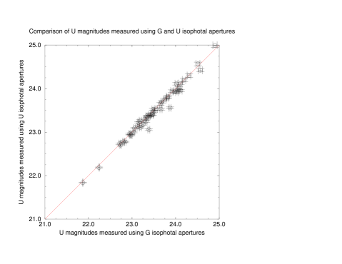
Figure 1: Comparison of $U$ magnitudes measured using isophotal apertures made from the $U$ and $G$ images. The objects shown here all have $21<R<22$ and $U<25$.

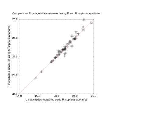
Figure 2: Comparison of $U$ magnitudes measured using isophotal apertures made from the $U$ and $R$ images. The objects shown here all have $21<R<22$ and $U<25$.

To check that the choice of isophotal apertures did not produce a systematic offset in the measured flux recorded from each image, we compared the magnitudes measured from isophotes based on each broadband image. Examples of these comparisons are shown in Figures 1 & 2. There is no evidence for a systematic offset in the magnitudes recorded between any of the isophotal apertures for the majority of the sample. However, it seems that occasionally, in five percent of cases at the most, objects have magnitudes which are sensitive to the choice of isophotal aperture. This is most marked in Figure 2, where some six objects show a greater difference in $U$ magnitude than can be accounted for by photometric errors. Since these colour–dependencies will only arise in resolved objects, this is only likely to affect those galaxies at low redshift. Additionally, we stress that the comparison between $R$ and $U$ is the most extreme case in this catalogue.

4.4 Determination of differential galaxy counts

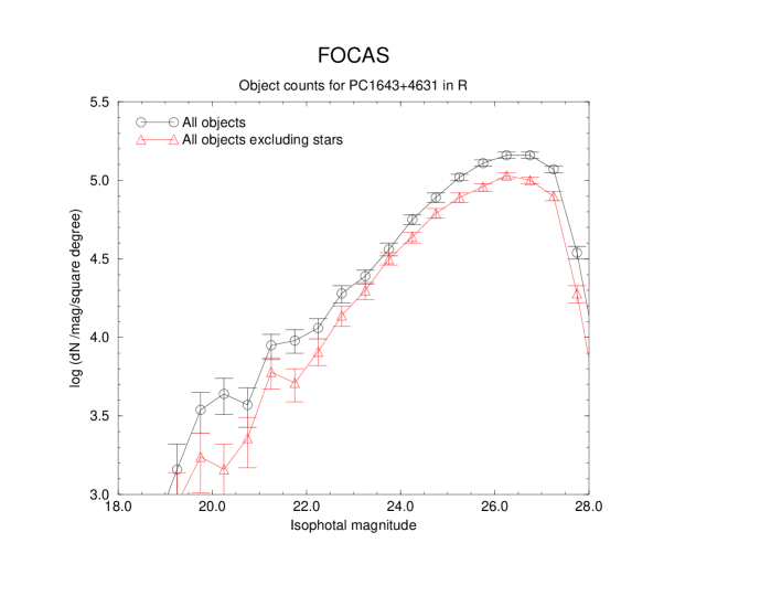
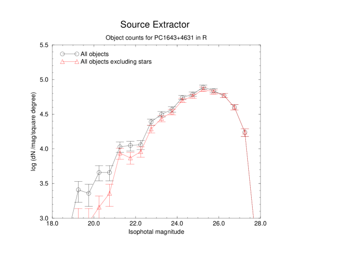
Figure 3: Comparison of the object counts before and after star rejection for FOCAS and SExtractor

To compare our imaging of the PC1643 field with other deep observations, we first investigated the differential galaxy counts. This requires that all stellar objects in the field are removed from the catalogues (see, for example, [Tyson, 1988] ), and the two programs use different approaches to stellar classification. The FOCAS software uses the point spread function to differentiate between stellar and non-stellar features and allocates a type to the object depending on the geometry of the object. SExtractor’s approach relies on a previously–trained neural network to assess the light distribution of the object and assigns a ‘stellar index’ to each object; this is a confidence estimate on the stellar-like nature of the object, ranging between 0 (galaxy) and 1 (star). We have taken all objects with a stellar index of greater than 0.8 to be stars and these objects have been excluded from the galaxy counts. The results of this procedure are illustrated in Figure 3.

Both these approaches to classification have difficulty at faint magnitudes – the SExtractor algorithm is unable to give high confidence levels for objects within about 2 magnitudes of the catalogue limit, as one might expect given the reduced signal to noise. FOCAS appears on the other hand to continue to classify very faint objects as stars almost down to the noise level – since many of the fainter galaxies are effectively unresolved, they appear as point–like objects and are misclassified as stars. FOCAS is therefore almost certainly overzealous in its allocation of stellar classifications, since for $R>24$ it classifies over half the objects as stars, whereas here one would expect the galaxies to dominate: the number of stars per unit area of sky is roughly equal to the number of galaxies per unit area of sky at 20th magnitude at high galactic latitude ([Bertin and Arnouts, 1996]). The very brightest objects, with $R<21$, are predominantly stars, although the increase in the total and galaxy–only counts at $R\sim 20$ is misleading since these objects are increasingly saturated in the CCD image for $R<20$, leading to an artificial excess of galaxy counts at this magnitude.

FOCAS appears to be capable of detecting more faint objects than SExtractor, as demonstrated by the magnitude at which the differential counts begin to turn over (Figure 3). This may be due to the differing approaches to splitting multiple objects employed by the catalogue programs – the magnitudes at which this effect is most noticeable are close to the limit of the images. Closer examination of the faintest detected objects in both catalogues suggests further possibilities. The validity of the faintest objects in the FOCAS catalogue is questionable, as there is a significant increase in the density of objects around the brightest stars in the image, where the background noise is higher. This is almost certainly due to the global threshold value above the background which FOCAS uses to determine its intensity threshold – in areas of higher background noise, such as around the brightest objects, the local rms noise level is higher, leading to a higher probability of the software identifying noise peaks as real objects.

SExtractor suffers difficulties in separating faint objects from brighter companions, even with the highest allowed level of contrast, and may therefore wrongly aggregate such objects together. This is most noticeable around the brightest stars in the image, where it fails to separate objects out of the wings of the stars, even on the most extreme contrast settings. Similarly, considerable care in setting the detection parameters is necessary to ensure that faint objects near to bright galaxies are correctly found.

4.5 Determination of photometric measurement errors

To quantify the ability of the software to recover galaxies from the field, we carried out simulations using artificial galaxies created with the IRAF package ARTDATA. This package allows the user to create and place galaxies with either de Vaucoleurs or exponential profiles in random, clustered or user-defined distributions with various magnitude distributions.

We followed two approaches. First, 100 sample galaxies with a 40:60 mix of ellipticals and spirals, of fixed magnitude and a comparable range of sizes to those in the actual image but otherwise random orientation and aspect, were added to a noise–only image. This noise–only image mimicked the background level in the actual field, including the raised background level around the stars. Second, model galaxies generated in the same way were also added directly to the real image. FOCAS was then used to perform the photometry on both the new images and the recovered fluxes were compared with the starting values.

As can be seen from Figure 4, there are significant differences between these two approaches. Recovery of objects from a noise-only image suffers from a serious discrepancy of as much as half a magnitude from the real magnitude (as indicated by the error bars in Figure 4), whereas the results of recovery of the simulated galaxies from the real field are, on average, much closer to the expected value. This is not a failure of the software to determine accurately the sky level surrounding the objects in question as demonstrated in Figure 5, since there is no evidence for the measured sky background level around the objects being a function of simulated magnitude. As expected, recovery from a real field shows a much wider spread of magnitudes due to contamination by neighbouring galaxies and this inevitably leads to an increase in the measured fluxes of the artificial objects. This confusion between between objects on the sky is almost certainly responsible for reversing the loss of flux beyond the isophotal apertures. Since this effect will occur for real as well as the simulated galaxies, using simulations based on recovery from noise-only images or mosaics significantly overestimates the loss of flux from the apertures.

The effects of confusion with faint sources in the field are most pronounced at the faintest magnitudes measured, resulting in a significant overestimate of the brightness of the source – the faintest sources show the greatest increase in isophotal magnitude when they overlap with real field objects. This is demonstrated in the $V$ and $I$ image simulations in Figure 6, where $I=25$ and $V=26$ galaxies are comparatively brightened on average. The $R$, $G$ and $U$ images are almost 1.5 magnitudes deeper than the $I$ observations and such effects are not seen in the range 22nd–26th magnitude.

In summary, it appears that using magnitude corrections based on detecting and performing photometry on simulated galaxies placed in a noise–only field suffers a significant systematic discrepancy when compared to recovery of similar galaxies from the actual image. This difference can be as high as 0.4 magnitudes for objects with low signal–to–noise. For these fainter objects, the presence of many brighter neighbouring objects counteracts the loss of flux from the edges of an object measured using isophotal apertures. It is also worth noting that in recovering simulated galaxies from the real image, the measured isophotal magnitudes show a greater spread of values about the simulated magnitude than those recovered from the noise image, further reinforcing that there is no evidence for the need to make any corrections to the isophotal magnitudes.

4.6 Completeness of galaxy counts

To estimate the completeness of the catalogue, we examined the ability of the software algorithms to recover sets of simulated galaxies added to the field. Although maximising the number of galaxies added in each iteration reduces computing time, it is important that the number of galaxies added is not so great that a significant number of galaxies overlap. We chose to add 100 galaxies per iteration: the probability of any two of these galaxies being coincident is approximately one percent and is therefore insignificant.

Accordingly, 100 simulated galaxies were added to the real image, with the magnitudes distributed to imitate the real distribution, and with the 40:60 elliptical/spiral mix as before. The indices of the power–laws were taken directly from the real raw galaxy counts for this field, and were based on linear regression of the linear section of the galaxy counts fainter than 20th magnitude. This procedure was repeated 20 times for each broadband image; this was enough to show clear trends.

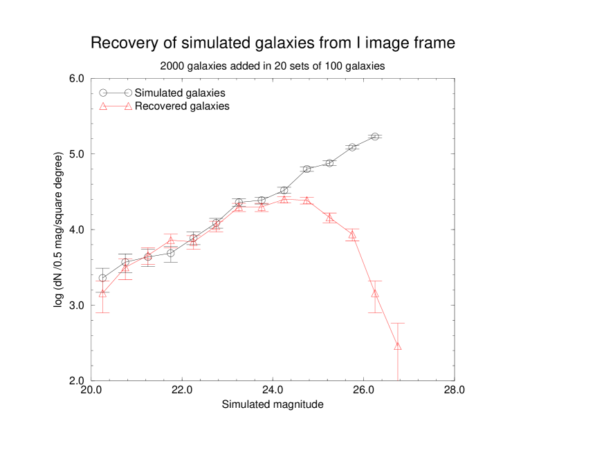
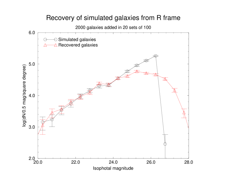
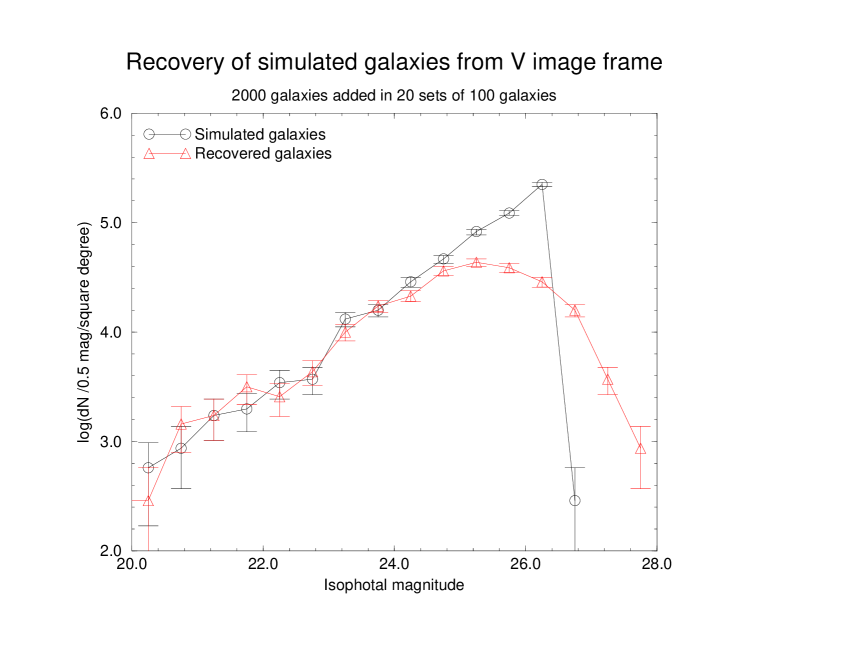
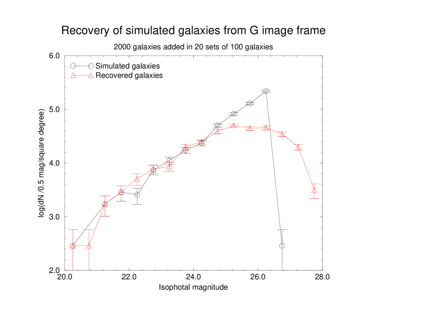
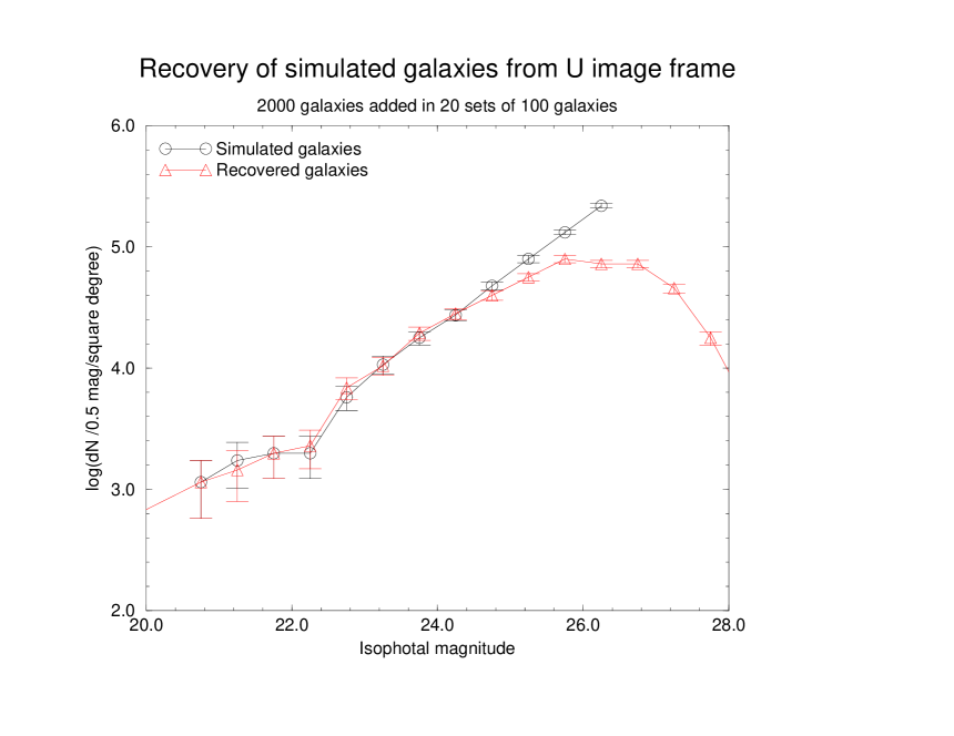
Figure 7: Simulations on the completeness of the five broadband catalogues

The results of these simulations (Figure 7) give direct information on the ‘loss’ of galaxies from their real magnitude bin. This loss occurs in two forms: failure to detect a faint galaxy, usually due to it falling below the surface brightness limits of the images; and failure to determine the magnitude of the galaxy to an accuracy of less than the bin width in the histogram, as explored in section 4.5.

It is worth noting that for the brighter end of the simulation, there is little or no deviation between the simulated galaxy magnitude histogram and that of the recovered galaxy histogram, entirely consistent with the accurate recovery of individual galaxies as seen in section 4.5. The point at which the catalogues become significantly incomplete (which we take to be as losing more than half the real number of galaxies) is tightly correlated with the accuracy with which the galaxy magnitude can be measured, and a completeness limit of roughly 50% is reached when the photometry errors reach a magnitude.

We also point out that these simulations are not suitable for accurately estimating the completeness of the catalogue at all magnitudes as they do not go faint enough, despite going close to the measurable limit of the catalogues. This is clearly demonstrated in the $U$ simulations, where the simulated $U$ counts turn over before the real $U$ counts do. If these simulations are used to attempt to correct the raw differential counts to the actual galaxy counts, the resulting counts are over–estimates because the simulations themselves do not cover all the real spread of magnitudes. Additionally, because these simulations rely on prior knowledge to provide a distribution from which to simulate the galaxy counts, there may be a tendency for the results of these simulations to merely confirm the starting hypothesis when the catalogues become markedly incomplete. In summary, unless the raw counts themselves are effectively complete, the corrections often made to the raw counts to account for the incompleteness may prove to be erroneous if the starting hypothesis is incorrect.

5 Images

A full–colour image comprising all the five broad band filters is shown in Figure 8. There is no obvious cluster in this field, which might be visible if the cluster were similar to a rich Abell cluster at a redshift of $z<1$ (cf [Luppino and Kaiser, 1997]) – such a cluster would have $I\approx 20$ for the brightest cluster member, and have several members brighter than $I\approx 23$. The band of bright objects across the centre of the field evidently consists of objects with several different colours and is therefore not a system at one specific redshift. The quasars A & B appear yellow in this image, which is due to the absence of any observed flux in $U$, and no unequivocal third image candidate is seen in this colour image, although there are some faint yellow objects in the centre of the field. It is also notable that the faintest objects are predominantly blue.

6 Differential Galaxy counts

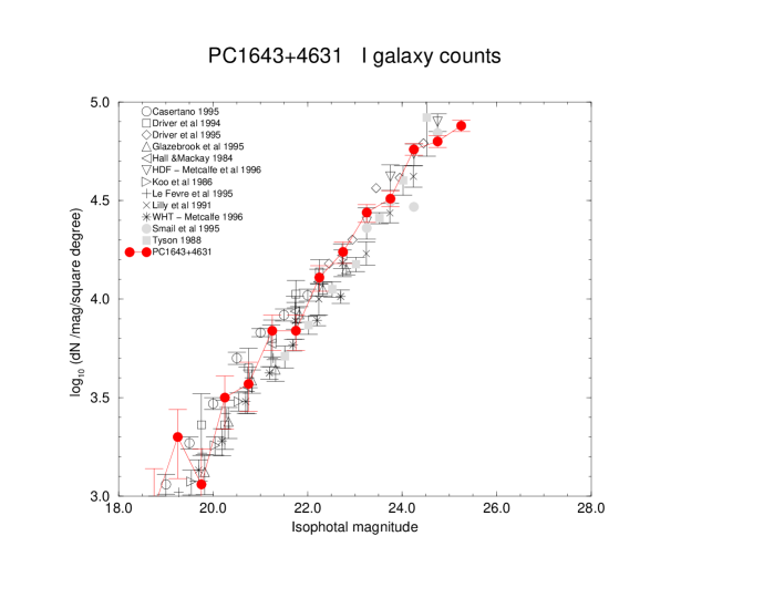
Figure 9: Galaxy counts for $I$ filters, compared with previously published results

I–band galaxy counts already exist for several fields. Figure 9 shows some of these together with the countes for PC1643; there is very good agreement. In Figures 10–13 we present the PC1643 counts in $R$, $G$, $V$ & $U$, with comparison counts where possible. Four points are of note:

1. The field of PC1643 is similar in its counts to all the other ground–based deep fields used in the literature for measuring differential galaxy counts. This is true in each broadband filter.

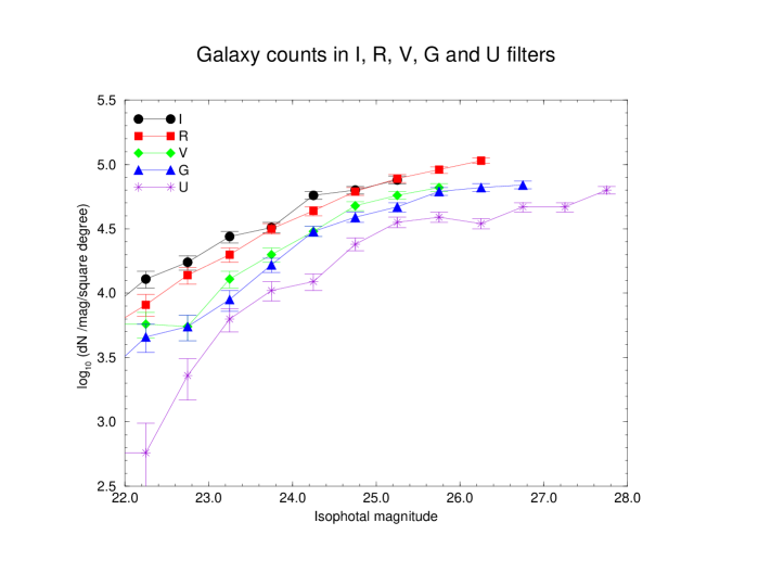
Figure 14: Galaxy counts for all broadband filters used here

2. Down to $\textrm{magnitudes}\sim 24$ the slope of the counts increases with decreasing wavelength, caused by the presence of the faint blue population which becomes a significant proportion of the sample at the fainter magnitudes. This is clearly seen in Figure 14. Beyond a critical magnitude, the counts fall off due to the difficulties in detecting the fainter objects above the pixel noise. No attempt has been made in these galaxy counts to ‘correct’ for these discrepancies.

3. Also clear is the flattening of the $U$–band counts at fainter magnitudes – this may be partly due to the Lyman limit of high–redshift galaxies at $z\sim 3$ moving into the $U$ filter, resulting in a drop in perceived counts.

4. It is noticeable that the results published by [Hogg et al., 1997] and [Songaila et al., 1990] continue to rise steeply where our counts level off at $U\approx 26$. Since our results are raw counts, this may be evidence of incompleteness in our sample. However, it is interesting to note that the $U_{300}$ counts published in [Williams et al., 1996] from the Hubble Deep Field do not continue to rise steeply past $U\approx 26$. The HST $U_{300}$ filter has a wavelength range of approximately from 2000Å to 4000Å  compared with ground–based $U$ filters which are effectively limited by atmospheric absorption to a shortest wavelength of approximately 3000Å. The $U$ bandpass (including the effects of atmospheric transmission, CCD response and telescope lightpaths) of these observations gives us a range from 3000Å to 4000Å, i.e. a subset of the HST bandpass. The greater range of wavelength of the HST $U_{300}$ observations means that the $U_{300}$ counts will start levelling off at slightly different magnitudes to the $U$ used here.

The method used here to test completeness, i.e. of comparing the expected differential counts with those actually recovered from the images, relies on the actual counts following the trend set out in the model – in this case, a power–law behaviour. Other completeness models (eg [Hogg et al., 1997]) also rely on there being no sharp changes in the slopes of the real differential counts. With the results of the HDF counts, we can be confident that this is indeed the case for the counts presented here, with the exception of the $U$ counts. It seems entirely feasable that this sharp change results in an overestimate of the counts compared with two “traditional” completeness estimators.

7 Searches for line emission using the narrow–band filters

We searched for candidates showing strong line–emission around $z=3.14$ & $z=3.81$ by comparison of the magnitudes of the objects in the narrow–band images against the magnitudes of the same objects in the broad–band images. Similarly we also searched for strong absorption at the two redshifts, such as is seen in the spectrum of Quasar A. Our search criteria was based on identifying objects which have $(\textrm{broadband}-\textrm{narrowband})$ colours which lie at least $4\sigma$ away from the expected continuum value. Additionally, these objects should be extremely faint in $U$, since the column density of neutral hydrogen will absorb any radiation below 912Å in the rest frame of the galaxy, and at a redshift $z>3$ this falls inside our $U$ filter. With the exception of the quasars there are no strong candidates with highly significant $(\textrm{broadband}-\textrm{narrowband})>6\sigma$ values. More marginal candidates exist with in both cases, with $(\textrm{broadband}-\textrm{narrowband})\approx 4\sigma$, $R\gtrsim 24$ and faint $U$ magnitudes.

7.1 Searches for galaxies at $z\sim 3.8$ using the L5840Å filter

Figure 15 shows the $R-L5840$ colours for catalogues based on $R$ and $G$ isophotal apertures constructed using FOCAS and SExtractor for comparison. The quasars are marked and are the only objects standing clear of the rest of the catalogue. The increase in photometry errors can account for the spread of the candidates at faint magnitudes, and the range of $G-R$ colours contribute to the spread of $R-L5840$ colours at all magnitudes. Choice of isophotal apertures or photometry software appears to make little difference, although there are more faint–magnitude objects in the FOCAS catalogues. Based on the FOCAS catalogue using $R$ isophotal apertures, we find 25 objects with $R-L5840>4.5\sigma$ in the range $19<R<26$. Of these candidates, eight objects (including the quasars) have $U-G>2$ suggesting that they may be at $z>3$.

The apparently increased scatter in $R-L5840$ suggesting absorption at 5840Å (ie increasingly negative $R-L5840$ values) is not significant, since the fainter $L5840$ magnitudes have larger photometric uncertainties. This also explains the apparent rise in the median $R-L5840$ values at $R>24$, since the fainter $L5840$ candidates are increasingly undetectable for the larger negative $R-L5840$ values.

7.2 Searches for galaxies at $z\sim 3.14$ using the S5040Å filter

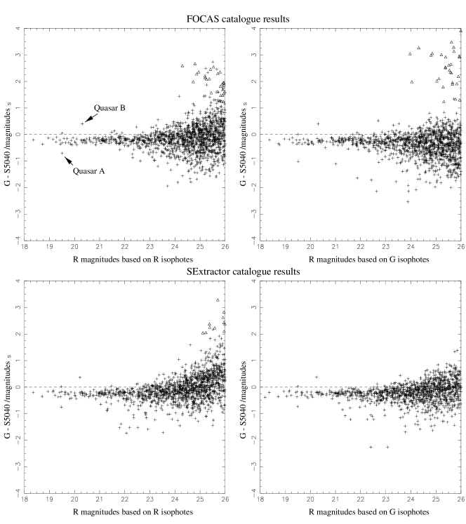
Figure 16: Broadband – narrowband magnitudes for the search for Ly-$\alpha$ emission at $z\approx 3.14$

In Figure 16, we plot the $G-S5040$ colours for catalogues based on $R$ and $G$ isophotal apertures constructed using FOCAS and SExtractor for comparison. Quasar A stands clearly out from the rest of the catalogue showing the Ly-$\alpha$ absorption feature. However, Quasar B shows a distinct excess over the G band. Examination of the spectrum of Quasar B ([Saunders et al., 1997]) reveals this is consistent – there is some emission between 4950Å and 5100Å over the contiuum level but this is almost certainly due to Ly-$\beta$ (perhaps with some OVI) emission from the quasar itself rather than Ly-$\alpha$ emission from an object at $z=3.14$.

In the range $19<R<26$ we find 70 objects with $G-S5040>3\sigma$ and 6 objects with $G-S5040>4.5\sigma$. Of the 70 objects, 3 have $U-G>2$. The differences between the FOCAS and SExtractor–derived catalogues at the faintest magnitudes ($R\approx 25$) shows a number of more extreme $G-S5040$ candidates for both sets of isophotal catalogues, but these objects have large photometric uncertainties.

In comparison with other narrowband searches for Ly-$\alpha$ emitters at $z>3$, we would have expected about 6 Ly$-\alpha$ emitters in a field this size ([Hu, 1998]). Our broadband images are sufficiently deep to have detected continuum from all but the faintest galaxies assuming a similar distribution to Cowie & Hu’s sample ([Cowie and Hu, 1998]). However, our narrowband images are not as deep and it is likely that there may be other faint galaxies with strong emission lines which are buried by the photometric errors. Given that $R-L5840\lesssim 1$ even for a strong Ly-$\alpha$ emitter, using objects detected in the much deeper broad–band filters rather than using catalogues based on isophotal apertures in the narrow–band images should not have missed a significant number of galaxies. The range of broadband filters we have here also allows us to discriminate strongly against other possible emission lines, such as [OII], by ensuring that the continuum measurements are consistent with Lyman–break high–redshift galaxies.

8 Colours and spatial distributions

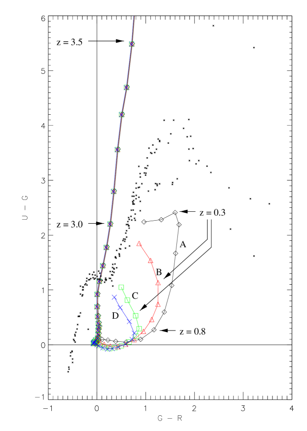
Figure 17: Simulated galaxy colours as a function of redshift. The crosses represent stars taken from the stellar database ([Gunn and Stryker, 1983]) ranging from about O5 to M3. These models are derived using a formation redshift $z_{f}=5.0$, using bc96_0p0200_sp_ssp_kl96.ised in the B&C 96 distribution. The various tracks A-D are based on the following star formation histories:

We used the GISSEL code developed by Bruzual & Charlot [Bruzual and Charlot, 1993] to model the colours of distant galaxies observed through our filters, in a similar manner to that adopted by [Steidel and Hamilton, 1993]. The standard evolution curves for three simulated galaxies in the $U-G$ and $G-R$ colours are shown in Figure 17. Note the close coincidence of all of these evolution loci beyond a redshift of 2.6, and the extreme red $U-G$ colours for higher redshift galaxies.

In general, trying to select objects at some redshift by optical colour is only efficient for specific redshift ranges. At low redshift, the 4000Å break provides a clear colour signature that can be used to identify galaxies between $0<z\lesssim 1.2$. Once the 4000Å break moves out of the $I$ band around $z\approx 1.2$, the continuum spectrum covered in the 3000Å – 9000Å range is fairly flat, making identification more difficult. This trend continues until the Ly–$\alpha$ forest and Lyman–break features move into the shorter wavelength filters at $z\approx 2.7$, resulting in a rapid faintening of the observed $U$ magnitude and providing a clear $U-G$ colour signature by $z\approx 3$. At still higher redshifts, the $U-G$ vs $G-R$ colour–colour diagrams would seem to suggest that identification of such galaxies would be equally efficient, and in the case of a extremely deep field, such as the Hubble Deep Field, this is observed. However, our data are limited to $R\approx 27$. As a result, any population of $3.5<z<4.1$ galaxies, with $R\approx 26$ and $G-R\approx 1$, are recorded with lower limits of $U-G\approx 2$ and are confused with the ‘body’ of the colour–colour diagram. For redshifts $z\gtrsim 4.1$, the Lyman–break has moved into the $G$ filter, and hence a similar search to that carried out for $z\approx 3$ galaxies can be done using $G-V$ vs $V-I$ or similar.

8.1 Intermediate redshifts

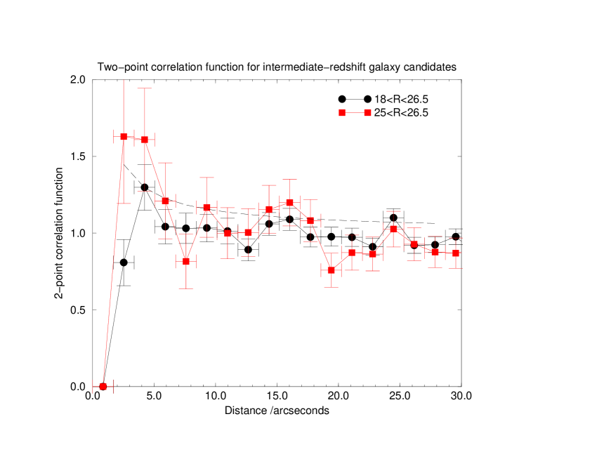
Figure 19: Two–point correlation function for the faint intermediate–redshift candidates

Objects in the field at intermediate redshifts, $1<z<2.5$, are likely to be very blue in $G-R$ (see Figure 17), although reddening of these galaxies may affect this colour difference. This also assumes that they are still vigorously starforming at these redshifts. Adopting limits of $0<(U-G)<2$,  $0<(G-R)<0.5$ and $R<26.5$ to limit contamination from low and high redshift galaxies as far as possible, we find a total of 494 objects with suitable colours in the central $5^{\prime}\times 5^{\prime}$ region, using the catalogue based on the $R$ isophotal apertures. Examination of the distribution of these objects on the sky reveals no visually discernable dense region. The two-point correlation function (given in Figure 18) for all of these objects shows that the field is indeed remarkably uniform, although there is a suggestion that there are more objects at the edge of the field than in the middle . Splitting the sample into magnitude–selected groups shows that there is more clustered structure at the brighter magnitudes, while there is evidence of small–scale ($<20$ arcsec) grouping of the candidates at the faint magnitudes (Figure 19). Fitting the standard power–law, $w(\theta)=A_{\omega}\theta^{-\beta}$, to the whole sample over angular scales $\theta$ from 2 – 30 arcseconds using non–linear curve–fitting gives close–to–zero values for $A_{\omega}$. Repeating this procedure for the faint end of the sample with $25<R<26.5$ gives best–fit parameters of $A_{\omega}\approx 3.3$ and $\beta\approx 1.6$, suggesting that these galaxies are more strongly clustered than galaxy samples in the local universe. Values of $\beta=0.8$ and $A_{\omega}\approx 0.9$ ([Brainerd and Smail, 1998]) can be well fitted with our data for angular scales less than 20 arcseconds, but diverge for larger scales at a 95% confidence level.

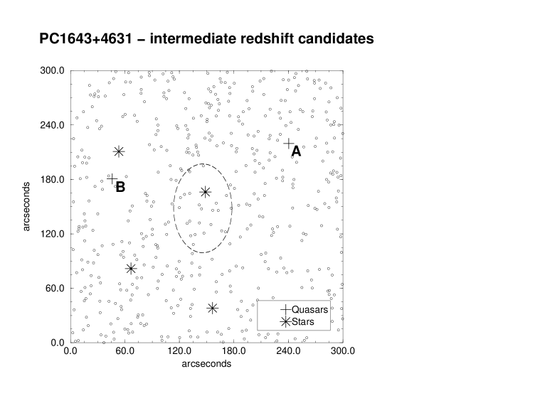
Figure 20: The spatial and magnitude distributions of the intermediate–redshift candidates, based on $R$ isophotal apertures. The dashed ellipse shows the $1\sigma$ limits of the position of the centre of the S-Z decrement. The bright candidates with $R<22$ are almost certainly blue stars contaminating the sample

As shown in Figure 20 the majority of these intermediate redshift candidate objects are at faint magnitudes in the range $24<R<26.5$ as expected; the 26 brightest objects with $R<22.5$ are almost certainly all stars. However the slope, $\textrm{dN}/\textrm{dm}$, of these objects between $22.5<R<25$ is higher than the slope of the whole sample (as shown in section 6) and is more consistent with the slope of the $G$ band observations.

The exact number of intermediate redshift objects found depends on the choice of isophotal apertures, as tabulated in Table 4. Selection from the $G$ isophotal apertures gives significantly (ie $3\sigma$ assuming Poisson statistics) more candidates than from the $R$ isophotal apertures despite the approximately equivalent magnitude limits of the images. Comparing the magnitude distributions shows that this discrepancy occurs mainly at magnitudes of $24<R<26.5$, suggesting that this effect is due to photometric measurement errors. Selection of objects using the $G$ isophotal catalogue results in more faint $R$ objects being included in the set. This may be due to the slightly larger isophotal apertures obtained from the $G$ images increasing the photometric errors. Comparison of these two matched catalogues based on isophotal $R$ and $G$ apertures against the matched catalogue using isophotal apertures made from each broad–band image for each filter suggests that, in this case, the $R$ isophotal catalogue is giving a more accurate set of results. While it would appear that using a catalogue where each image uses its own isophotal set of apertures is optimal, particularly since there is no guarantee that the isophotal apertures need be colour independent, using $R$ isophotal apertures is more effective here for several reasons:

1. the surface brightness limit of the $R$ image is fainter than the other frames, with the exception of $U$;

2. by detecting objects in $R$, objects in filters bluer than $R$ are unlikely to be missed, which is the main reason not to use $U$ for the isophotal apertures (e.g. Lyman–limit galaxies are not detected in $U$);

3. where objects in less–deep images would not be recognised at all using isophotes based on that image, using isophotal apertures based on the deeper $R$ frame allows upper limits to be places on the magnitude of that object.

8.2 High redshifts

We next investigated candidate Lyman–break galaxies at $z\gtrsim 3$. Using the same approach as Steidel and Hamilton (S&H), we have included objects which have $R<25.5$ (ie $R\gtrsim 10\sigma$) and are detected in $G$ to at least $2\sigma$. We then selected ‘robust’ candidates as having $U-G>2.25$, $G-R<1.25$ and $(U-G)>4(G-R)+0.5$ as illustrated in Figure 21. A second set of looser criteria to include more ‘marginal’ detections was also used, requiring $U-G>2.0$, $G-R<1.25$ and $(U-G)>4(G-R)$. These are slightly different to the colour selection criteria used by Steidel and Hamilton, and reflect the differences between the filters we used and S&H’s – most noticeably the track of stars (taken from the Gunn & Stryker atlas) runs at bluer $G-R$ colours than through the Steidel filters and our $U-G$ colours are redder than those of S&H’s for the same galaxy at a similar redshift. We stress that the colour criteria we use are at least as conservative as that adopted by Steidel et al.: the lower limit on $U-G>2.25$ cuts across the B&C tracks at $z=3.0$, whereas the ‘robust’ Steidel criteria selects at $z\approx 2.85$ (see eg [Steidel and Hamilton, 1993]). Similarly, by using $(U-G)>4(G-R)+0.5$, contamination from any stars is minimised: the photometric errors for typical Ly–limit candidates with $R\approx 25$ do not extend to those colours consistent with stars, whereas the criteria of Steidel et al. include stars with $U_{n}-G\approx 1.0$ and $G-\mathcal{R}\approx 2.5$ (see [Pettini et al., 1997]).

We have identified 27 robust candidate high–redshift galaxies in the central 5’x5’ of our images, and a further 12 marginal candidates. The two extreme $U-G\sim 7$ objects in the field are Quasars A & B. Of the robust candidates, only 7 have detections in $U$ of at least $1\sigma$, while 6 of the marginal candidates have $U$ detections of $1\sigma$, with at least one being almost certainly a star. The magnitude distribution for the robust candidates is plotted in Figure 22, and shows that, with the exception of the two quasars, all the objects have $R>23.5$, consistent with the findings of Steidel et al.

We would expect to find 10 $U$–dropout galaxies with $R<25.0$ assuming a surface density of 0.4 per square arcmin ([Steidel et al., 1996])—and assuming Poisson-distributed galaxies—and find 11. However, on lowering the limit to $R<25.5$, [Steidel et al., 1998] reports a mean surface density of $\approx 0.7$ and so we expect only 7 with $25.0<R<25.5$ but find 16 candidates – a 3-$\sigma$ excess.

Comparison of the 27 candidates with $R<25.5$ in the central $5^{\prime}\times 5^{\prime}$ area with the surface density $\approx 0.7$/square arcmin for the SSA22 [Steidel et al., 1998] field implies that we have a excess of faint high–redshift objects in the field of PC1643.

Typical photometric measurement errors in $R$ are of the order of 0.05 magnitudes, with the uncertainty in the $G$ measurement being closer to 0.1 magnitudes. This is not sufficient to drastically affect the number of candidates included inside the criteria. Even allowing for the additional errors due to photometric measurement, the robust candidates are at least $1\sigma$ away from the stellar track in both $U-G$ and $G-R$. This is consistent with the approach adopted by S&H.

Using the different isophotal catalogues available has some effect on the colours recorded for the candidates derived from the $R$ isophotes. Table 5 shows the fraction of the 27 candidates which are well matched in position to positions in the different catalogues, along with the number which still fulfill the original criteria for selection. Where cases have not fulfilled the colour criteria, this is mainly because the isophotal apertures have been taken from the less deep images, such as $V$ and $I$. The deviation in the case of the $U$ isophotal apertures is due to the strong colour dependance of this selection criterion.

Most of the photometric uncertainty is in the determined value of $U-G$, particularly the determination of the $U$ magnitude. Individual scrutiny of the candidates indicates that some 10 candidates show faint but discernible flux in $U$, and it would appear that these detections can be supported by matching the positions of the apparently $U$ devoid candidates against the catalogue based on the $U$ isophotal apertures. Because galaxies beyond $z\approx 3$ will show significant extinction of photons below the Lyman–limit, such candidates with $U$ flux are more likely to be at redshifts of less than 3. However, it is worth noting that Quasar A has a close companion within $2^{\prime\prime}$ with significant $U$ flux, underlining the fact that the discarding of high-redshift candidates by this method may actually remove real high-redshift objects through line–of–sight confusion with foreground objects.

Examination of the positions of the 27 high–redshift candidates on the sky shows a distinctly non-random distribution (Figure 23). The region between the quasars appears to be sparse in candidates – taking a circle of radius 80” about a position midway between the two quasars yields no objects, while an annulus extending from 80” to 160” contains 20 objects. If the objects in the field were uniformly distributed, one would expect 5 objects in the central circle and 15 objects in the outer annulus. Applying a $\chi^{2}$–test to these data gives $\chi^{2}=6.6$ with 1 degree of freedom, which corresponds to a probability of $>0.95$ that this distribution is not consistent with a uniform distribution. The contrast with Figure 20, the intermediate–redshift candidates, is marked.

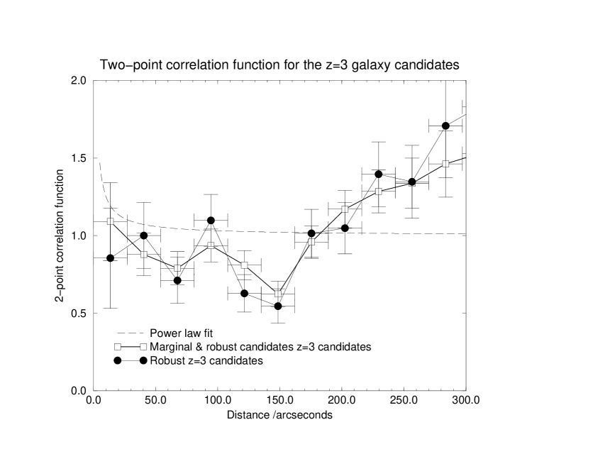
Figure 24: Two–point correlation function for the high–redshift candidates

We plotted the two–point correlation function, $\omega(\theta)$, for the 27 high–redshift candidates (Figure 24) which shows clustering on small scales and anti–correlation on scales of $\approx 100^{\prime\prime}$, as expected given the lower surface density in the centre of the field. The apparent clustering at $250^{\prime\prime}$ scales is due to the characteristic length of separation of the sample across the void. We plotted the best fit power–law as determined from the sample of 871 Lyman–break galaxies ([Giavalisco et al., 1998]), finding $A_{\omega}=2\textrm{arcsec}^{\beta}$ and $\beta=0.9$, which is an extremely good fit to our data here on scales shorter than 80 arcseconds. We tested random distributions of points and determined that these features are not edge effects and are most unlikely to have occurred by chance.

Overall, the field towards PC1643+4631A&B appears to be at least as densely populated as the most densely clustered $5^{\prime}\times 5^{\prime}$ areas of the SSA22 field, which covers $8.6^{\prime}\times 17.6^{\prime}$. The presence of a void in PC1643, with an area of 7 square arcminutes in the centre of this field, appears unusual in comparison with SSA22.

It is difficult to determine whether this region does in fact have a high–redshift structure based on this information alone – the ‘wall’ at high-redshift found by Steidel et al following spectroscopy has an angular size of at least 10 arcmin, about twice the field of view on our images. However, the discovery that that the SSA ‘cluster’ lies at the same redshift as one of the quasars in that field is consistent with the hypothesis that quasars act as markers of large–scale structures at high redshifts, and that a similar correlation could be present in the field of PC1643+4631.

The distribution of Lyman-break candidates, with an apparent deficit between the quasars, could give rise to an apparent diminution of radio surface brightness if all the Lyman-break galaxies are sufficiently radioluminous, with 15 GHz flux $>20\mu$Jy, equivalent to $>40\mu$Jy at 8 GHz. However, extremely deep 8-GHz VLA imaging of the Hubble Deep Field (RIchards et al. 1998) detects no Lyman-brak galaxies with a 5-$\sigma$ upper limit of 9$\mu$Jy. We conclude that such a mechanism is not the cause of the microwave decrement.

8.3 A third image of the quasar?

Under the hypothesis that the two quasars PC1643+4631 A & B are indeed the same object gravitationally lensed by a $10^{15}M_{\odot}$ cluster of galaxies, we might expect to find a third image of the quasars in the images taken. Such a third image would have the same colours as the quasars (assuming no change of reddening), though if the third image passes close to another system this might make the colour signature unrecognisable. If A & B are indeed magnified images of a single quasar, then the third image should be demagnified and lie closer to the centre of the S–Z detection (see, eg [Schechter et al., 1998] and [Keeton and Kochanek, 1998]).

To identify suitable candidates for the third image, we compared the colours of Quasar B, which does not appear to have any nearby companions on the sky which might pollute the isophotal aperture, to all the catalogued objects detected in the $R$ isophotal catalogue. The most obvious approach was to examine the various colour–colour diagrams, particularly $U-G$ vs $G-R$ since this allows the more extreme $U-G$ colours of high–redshift galaxies to stand out from the rest of the objects in the field. As can be seen in Figure 21 there are no candidates with such extremely red ($(U-G)\gtrsim 5$) colours. This immediately gives us an upper limit on the brightness of the third image, assuming that its colours are not confused with a line–of–sight galaxy/star, of $R\sim 22$; i.e. three magnitudes fainter than the quasars themselves.

By comparing all the independent colours (i.e. $U-G$, $G-V$, $V-R$, $R-I$, $S5040-G$ and $L5840-R$) available for all the objects against Quasar B, we can obtain a collection of candidates for the third image. We used the statistic

$$\chi^{2}=\sum_{F}\frac{(F_{i}-F_{0})^{2}}{\sqrt{\sigma^{2}_{i}+\sigma^{2}_{0}}},$$ (1)

where	$F_{0}$ =	colour of quasar (e.g. $U-G$, $G-V$, etc),
	$F_{i}$ =	colour of object for comparison,
	$\sigma^{2}_{0}$ =	variance of colour of quasar,
and	$\sigma^{2}_{i}$ =	variance of colour of object,

to select the most similar objects, and included the known errors in measuring the photometry (as discussed in section 4.5) as well as the actual statistical magnitude errors based on the counts received inside the aperture. There are 7 candidates with $22.0>R>26.0$ which have a $\chi^{2}<5.0$, equivalent to 95% confidence limit.

The errors in measuring faint objects near the limits of the catalogue are significantly larger than the apparent statistical error; for example, at $I=24$, the typical statistical errors ascribable to Poisson errors in the background and aperture measurements are of the order of 0.1 magnitudes, while the error due to measuring these faint galaxies is of the order of 0.75 magnitudes. The search criteria therefore tend to pick out the faintest objects in the field since these produce significantly smaller values of $\chi^{2}$.

None of the objects selected is within the expected area of the sky for a gravitationally lensed third image, given reasonable modelling of the lensing potential constrained by the CMB decrement. However, the lack of an obvious third image by no means rules out the gravitational lensing hypothesis – examples exist in the literature of failed searches for a third image where the lensing hypothesis is better constrained than here, such as the first FIRST gravitationally lensed quasar ([Schechter et al., 1998]) and the double quasar Q2138-431 ([Hawkins et al., 1997]). (The demagnification of the third image may be as severe as to result in an image 5 or more magnitudes fainter than the quasars [Surdej et al., 1997]). The most probable reason for the absence of an obvious third image is that it is confused with another object in the line of sight.

8.4 Extremely Red Objects

Hu & Ridgway have discovered two extremely red objects (EROs), HR10 & HR14, within 1 arcmin of Quasar A ([Hu and Ridgway, 1994]). These were interpreted as being dusty galaxies at an estimated redshift $z\approx 2.5$ according to analysis of the colours, with HR10 however having a spectroscopic redshift of $z=1.44$ ([Graham and Dey, 1996]). We have compared our new optical observations with our previous infrared observations ([Saunders et al., 1997]) to investigate EROs in the other regions of the field. Our J and K observations cover about 15 arcmin² of the field, consisting of 7 pointed observations mosaiced together. The limiting AB magnitudes are $J\approx 22.1$ and $K\approx 18.1$ (corresponds to $J\approx 23$ and $K\approx 20$ Johnson magnitudes).

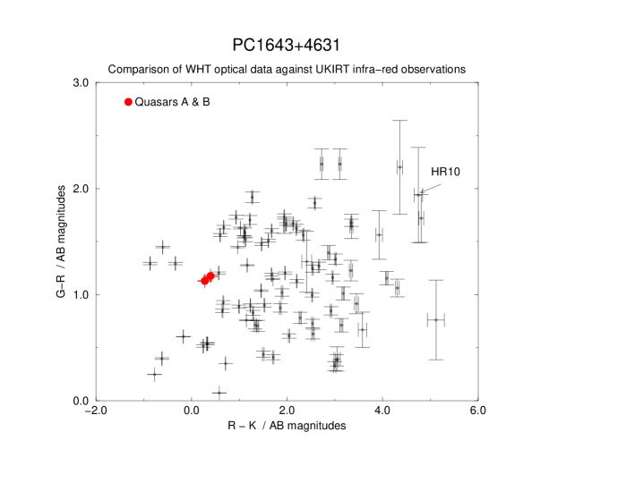
Figure 25: Comparison of optical colour against infra–red colour.

In Figure 25 we have plotted the optical colour against the infrared colour. There are 18 objects with $R-K>3$, all of which have $R>22$ (note that $R-K=3$ in the AB magnitude scheme corresponds to $R-K=4.6$ in Johnson magnitudes); their SEDs are plotted in Figure 26. Examining the $G-R$ and $U-G$ colours against the simulations based on Bruzual & Charlot algorithms suggests that none of these fall into the high–redshift category defined in section 8.2, being either too red in $G-R$ or being too blue in $U-G$ (see Figure 28). More critically, almost all of them have measureable $U$ flux which would not be present if we were imaging below the Lyman limit of these galaxies. All those objects which have no measurable $U$ flux are at the faint limit of the catalogue in $G$.

Note that while these objects have extreme $R-K$ colours, their optical colours are unremarkable ($G-R\approx 1$) and indistinguishable from the rest of the catalogue. If we take an E/S0 galaxy SED, such as that in Coleman, Wu & Weedman and examine the $R-K$ colours as we change the simulated source redshift, once the 4000Å break moves between the $R$ and $K$ filters at $1.2<z<2.5$, we obtain extremely red $R-K$ colours, peaking around $R-K\approx 4.8$ at $z\approx 2$. At this redshift, the $G$ and $R$ filters are measuring the small amount of UV flux in the E/S0 system, and have $G-R\approx 1$, consistent with the observed values here.

If the galaxy is undergoing star formation, the UV flux rises dramatically, and to acheive the $R-K\approx 5$ colours requires significant reddening. If all galaxies at $z\approx 2$ have a significant amount of star formation, then the degree of reddening required to produce the $R-K\approx 5$ colours would result in further reddening of the $G-R$ colours. Assuming a power–law reddening curve, where $\textrm{extinction}\ \propto\ \lambda^{-1}$, $\Delta(G-R)/\Delta(R-K)\approx 0.4$. Given the $G-R$ colours and the simulated galaxy colours derived from the Bruzual & Charlot models, this would suggest that extinction E($R-K$)$\approx 2$. This is assuming a uniform dusty extinction screen; it is more likely to be clumpy ([Witt et al., 1992]) with the result that significant reddening of the $R-K$ colours is possible while maintaining the $G-R\approx 1$ colours.

To summarise, an ERO need not be a remarkable object. It can simply be an E/S0 at $z\approx 2$. Or if most galaxies at $z\approx 2$ are star–forming, reasonable amounts of reddening may in practice give the observed spectra.

8.5 HR10 and other galaxies with $R-K>4.5$

We next compare our HR10 magnitudes with those already published ([Hu and Ridgway, 1994]). HR10 is clearly detected in our $I,R$ & $G$ filters, and marginally in our $V$ filter given prior knowledge of its shape and position from the other images. Because the magnitude of HR10 is faint in all filters, the automated photometry routines are less reliable than manual measurements, and it is these manual measurements which are presented in Table 6. Where no detection is made, $3\sigma$ upper limits are given.

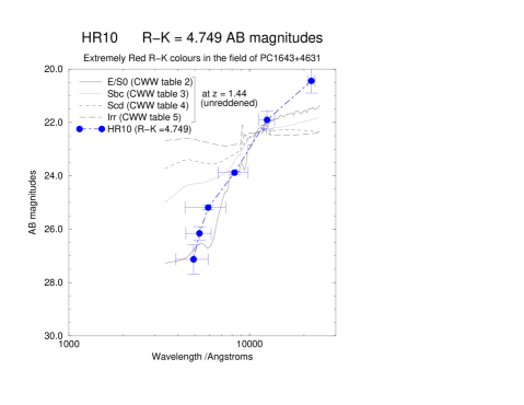
Figure 27: The photometry for HR10 compared against the redshifted CWW SEDs

The $z=1.44$ redshift of Graham & Dey for HR 10 is consistent with these colours. In Figure 27 we plot the SED from HR10 against the redshifted SEDs from CWW. The extremely good agreement of the HR10 colours with that of the E/S0 galaxy is intriguing. Compared with the B&C models of galaxy colours for a galaxy forming at $z=5$, one would expect the colours of an unreddened $z=1.5$ galaxy are $U-G\approx 0$ and $G-R\approx 0$ – ie extremely blue regardless of morphology. Dust scattering models where $E_{\lambda}\sim\lambda^{-1}$ result in reddening with $(\Delta(U-G))/(\Delta(G-R))\approx 1.8$. For $E_{\lambda}\sim\lambda^{-4}$, equivalent to Rayleigh scattering, reddening is more severe in $U-G$: $(\Delta(U-G))/(\Delta(G-R))\approx 4.4$. The non-detection of HR10 in the $U$ image is sufficient to give $U-G>2.0$ at the $1\sigma$ level.

The PC1643 data reveal two new objects with $R-K$ colours even more extreme than HR10. Comparing the SEDs of these against the CWW models suggest that they are also well fitted by an E/S0 spectrum at redshifts of $z\approx 1.7$. However, it is not possible to determine whether these objects belong to a cluster of galaxies at this redshift: the redshift determination, even with 7 broadband filters stretching from 3000Å to 24000Å, cannot be done to better than $\Delta z\approx 0.1$ and therefore determining whether these objects could be physically associated in some structure cannot be done with any accuracy from these data.

Little can be said about the morphology of the EROs observed here, as the seeing is too great to resolve a significant fraction. All have angular sizes of $1.5^{\prime\prime}$ or less, consistent with the FWHM$=0.7^{\prime\prime}$ for HR10 and HR14 ([Hu and Ridgway, 1994]).

Figure 29 indicates that the distribution of the EROs on the sky is not uniform but rather appears to be clustered into two main groups. The first group is in the upper half of the field and includes HR10, while the second group is in the lower half. Since the $K$ and $J$ observations do not cover the whole area of these optical observations, it is difficult to draw strong conclusions from this distribution. However, treating each of the $K$ images as a randomly–chosen independent area of sky (which is almost true – only the small areas of overlap are a problem here), one can estimate whether this distribution is consistent with a random distribution. Table 7 shows the number of candidates in each field. The field numbers used here are the same as in [Saunders et al., 1997].

There are 24 objects apparent in 7 fields – therefore the mean number of objects per square is $24/7\approx 3.4$. Using this as the expected number of objects per field, we obtain a value of $\chi^{2}=15.15$. There are 6 degrees of freedom, and hence the probability that this field is sampled from a uniform random distribution is 0.019 – ie this distribution is not consistent with a uniform random distribution at the 98% confidence level.

9 Additional discussion

From the full colour image alone, the lack of any visually obvious clustering of similarly coloured objects is enough to suggest that whatever system we are dealing with here is either extremely faint, with the majority of the member galaxies having $R\gtrsim 24$, or has only a few luminous members which are confused with the other galaxies in the field of view. Given the mass estimate derived from the S–Z detection, a normal Abell-like cluster of the same mass as Coma should be a distinct feature in these images if it were at $z\approx 1$ (cf [Luppino and Kaiser, 1997]).

In section 8.2, we have found a 3-$\sigma$ excess in the number of $z\approx 3$ galaxies in the field, as well as an indication of a diminution between the quasars. There would seem to be some bias operating in this field. Gravitational lensing by a system of $10^{15}M_{\odot}$ at $z\approx 2$, that also produces the CMB decrement, would produce these features. The seeing ($\approx 1^{\prime\prime}$) of the present observations would mask the weak shear of the background galaxies that would be present.

We also consider the possibilty that a proportion of these high–redshift objects is also at $z\approx 3.8$. Given the magnitude limits of these observations, it is unlikely that many galaxies at such a redshift would be visible in our images unless there is significantly greater star–formation at these redshifts that that found in previous high–redshift Lyman–break samples.

If the cluster of galaxies responsible for the S-Z decrement is dark, other techniques for its detection must be examined. A rich cluster of galaxies will gravitationally lens any background objects in the line of sight and affect the differential galaxy counts as a result ([van Kampen, 1997],[Broadhurst et al., 1995]). Given the variations of real galaxy counts from field to field, and along the line–of–sight, it is in this case impractical to apply this sort of analysis to this data. Since this system lies at high redshift, the difficulty lies in identifying what the real background population of galaxies at suitable redshifts (ie beyond $z\sim 2$) must be – the photometric uncertainties at these faint levels consistent with this population ($R\gtrsim 25$) are enough to statistically invalidate any strong hypothesis based on galaxy counts or colour–colour information.

Following the gravitational lensing theory further, the same background galaxies should show some shear distortion about the cluster position. Out of the images presented here, only the $R$ image is sufficiently deep to provide any hope of detecting shear in a high redshift population. However, these galaxies are all small – typical aperture size at $R=25$ is of the $\lesssim 30$ pixels at a 3-$\sigma$ threshold isophotal level – and the seeing is too poor to extract any useful shear information out of the field.

10 Conclusions

We have obtained deep multicolour images of an area of $5^{\prime}\times 5^{\prime}$ in the direction of the double quasar pair PC1643+4631 A& B and the CMB decrement. We have produced differential galaxy counts in five broadband filters, which are consistent with other published results, to $I<25.5$, $R<26.0$, $V<26.0$, $G<27.0$ and $U<28.0$. In doing so:

1. We find no cluster evident in contrast with the background. The distribution of galaxies in the image appears to be uniform within a 95% confidence limit. Given that the CMB decrement is most probably caused by a cluster of galaxies, such a cluster must either: (a) be indistinguishable, either in colour or distribution, from the other galaxies in the line of sight requiring that the over–density of galaxies in the cluster is a small signal; or (b) be at lower redshift and consist of too few luminous members to provide any contrast.

2. Colour selection indicates there are some 500 intermediate redshift ($z\approx 1.5$) galaxies candidates in the field. The distribution of these galaxies on the sky appears uniform.

3. We have detected 27 Lyman–break galaxies at $z\approx 3$ with $R<25.5$, of which 16 have $25.0<R<25.5$. This represents a 3-$\sigma$ excess over that expected for a $5^{\prime}\times 5^{\prime}$ field assuming Poisson-distributed galaxies with Steidel’s apparent average surface density of $0.7~{}\textrm{gals}/\textrm{arcmin}^{2}$ for $R<25.5$ and $0.4~{}\textrm{gals}/\textrm{arcmin}^{2}$ for $R<25.0$, even though the criteria we use to select the Lyman–break galaxies is at $least$ as conservative as Steidel et al.

4. However, the distribution of the Ly–break galaxies is inconsistent with a uniform one at the 2-$\sigma$ level. Rather, there appears to be a hole in their distribution positioned approximately midway between the two quasars; certainly there is no concentration of Ly-break candidates towards the either the quasar midpoint or the CMB decrement. The two–point correlation function for the Lyman–break candidates in this field is consistent with other published results on scales $<60$ arcsecs.

5. Points (3) & (4) are consistent with a model in which the S–Z effect is caused by a massive system of $10^{15}M_{\odot}$ at $z\approx 2$. This would also result in gravitational lensing of the background objects, including the quasars and the Ly–break galaxies, and is consistent with the distribution of the Ly–break galaxies in this field. Points (3) & (4) are also consistent with a genuine clustered system of Ly-break galaxies.

6. In a search for a third image of the quasars, several faint candidates were identified with consistent colours in the images; none of the objects is within the expected area of the sky for a gravitationally lensed third image. However, this does not affect the gravitational lensing hypothesis: the third image may be confused with or reddened by some object in the line–of–sight, or be too faint to detect.

7. A search for galaxies at $z=3.14$ and $z=3.81$ using custom–built narrow–band filters identified 3 and 6 faint candidates respectively.

8. We identified 18 EROs with $R-K>3$ AB magnitudes, and the distribution of these on the sky does not appear to be uniform. We find evidence for a population of red galaxies consistent with those found in sub–mm observations but reddened out of surveys in optical wavelengths.

9. The galaxy counts for this field, which are compatible with other published results, including the Hubble Deep Field. The $U_{300}$ counts from the HDF match the PC1643 raw $U$ counts more closely than the corrected $U$ counts of Hogg et al, and others. We suggest that this may be due to assumptions made by the algorithms used to correct for completeness, as in [Hogg et al., 1997] and [Songaila et al., 1990].

We have carried out simulations to measure the performance of commonly used object–finding algorithms and to investigate the possible biases in galaxy counts and catalogues. These show that:

1. simulations testing the completeness of the catalogues show that the magnitude at which the characteristic turn–over in the raw differential galaxy counts occurs due to incompleteness can be estimated from such simulations.

2. To obtain sensible estimates of the corrections needed to the differential counts, such simulations should go at least a magnitude deeper than the faint limit of the plate. Estimations of the “true” differential galaxy counts are biased towards the assumptions used to create the simulations. Therefore, important features in the differential galaxy counts will not be seen unless the raw differential counts are effectively complete at those magnitudes.

3. FOCAS appears to be more efficient at detecting faint objects than SExtractor. FOCAS also appears to be superior at subdividing composite objects where faint components adjoin a much brighter companion. However, SExtractor’s morphological classification appears to be more reliable than FOCAS, particularly for faint objects near the resolution limit.

4. Choice of isophotal aperture appears not to have a strong effect on the detection of Lyman–break galaxies, with both $R$ and $G$ isophotal apertures giving similar results. Similar results are also observed with different colour selection criteria, suggesting that the object shape and size is not a strong function of colour.

Finally, we have analysed the amount of flux lost from objects measured using isophotal apertures. We used two sets of simulations involving recovery of artificial galaxies from both the real image of the field and a noise–only image. These show that:

1. recovery of artificial galaxies from the noise–only image significantly over–estimates the flux lost from the object, and we find that corrections made using such a technique suffer a significant systematic error ($\approx 0.4$ magnitudes) as a result.

11 Acknowledgements

We would like to acknowledge the support from the staff at the WHT. The WHT receives funding from PPARC. TH acknowledges a PPARC studentship. GC acknowledges a PPARC Postdoctoral Research Fellowship. We would like to thank Richard McMahon for the loan of the $G$ filter used in these observations.

Filter	Exposure time /s
	15 April	16 April	17 April	18 April
$U$	6,300	—	3,600	2,700
$G$	—	3,000	—	—
$V$	—	1,200	—	993
$R$	2,700	—	4,500	—
$I$	—	—	—	2,700
$L5840$	1,800	2,400	—	—
$S5040$	—	—	—	1,800

Table 1: Observing log for 15 – 18 April 1996

Filter	Exposure	Zero–point	RMS noise	3$\sigma$ faint magnitude
	time (total)	magnitude	of image	limit for $2^{\prime\prime}$ radius
	/second		/ADUa	circular aperture
$U$	12,600	25.067	5.99 $\pm$ 0.2	27.01
$G$	3,000	25.938	14.3 $\pm$ 1.0	26.49
$V$	2,194	26.117	17.5 $\pm$ 1.2	26.01
$R$	6,600	26.324	20.1 $\pm$ 1.2	26.51
$I$	2,700	25.719	22.2 $\pm$ 0.9	25.04
$L5840$	4,200	23.861	13.5 $\pm$ 0.8	24.92
$S5040$	1,800	23.769	5.16 $\pm$ 0.3	25.43

Table 2: Calibration information for the PC1643+4631 images presented here. Note that seeing is $\approx$ 1.1 arcseconds FWHM for all images except $U$ where it is $\approx$ 1.5 arcseconds.

^a Analogue to Digital Unit – the number of electrons per ADU is described by the gain, which is 1.6 $e^{-}$/ADU for all observations, except those in $U$ where the gain is 1.2 $e^{-}$/ADU

Filter	50% complete
	magnitude limit
$U$	26.0
$G$	25.5
$V$	25.3
$R$	25.6
$I$	24.6

Table 3: Completeness limits for the broadband filters

Isophotal	Number of intermediate
aperture	redshift candidatesa
$U$	501
$G$	592
$V$	547
$R$	494
$I$	468
Self	460

Table 4: Completeness limits for the broadband filters

^a Using $R<26.5$, $0<G-R<0.5$ & $0<U-G<2$ in all cases

Isophotal	Number of candidates matched	Number fulfilling
aperture	to isophotal apertures	colour criteria
	within 1.6”
$U$	11	5
$G$	26	20
$V$	26	14
$I$	22	10
Self	27	18

Table 5: Comparison of the positions and colour selection criteria of high–redshift galaxies, based on the criteria outlined in section 8.2

Filter	Magnitude /AB
$U$	$>$27.	7 $\pm$	0.	7
$G$	26.	5 $\pm$	0.	5
$V$	$>$26.	0 $\pm$	0.	5
$R$	25.	6 $\pm$	0.	4
$I$	24.	5 $\pm$	0.	4

Table 6: AB magnitudes for HR10

Field	Number of candidates
0	1
1	7
2	3
3	1
4	4
5	2
6	4
Apparent total	24

Table 7: There are 7 slightly overlapping observations in K. These have the following number of EROs (classified as having $R-K>3$). There are 18 individual candidates, some of which appear in more than one frame, hence the larger apparent total.

The error bars on the counts are derived from the number of objects in each magnitude bin assuming a Poisson distribution.

Figure 4: Comparison of the recovery of simulated galaxies from real (left) and noise-only (right) images in R. The error bars shown here are the standard deviation of the magnitudes of the recovered galaxies from the original magnitudes, and do not take into account the skewness of the distributions. The lines merely join the means of the distributions.

Figure 5: Comparison of the recovery of sky level around simulated galaxies from real (left–hand figure) and noise-only images in $R$

Figure 6: Recovery of simulated galaxies from actual $U$,$G$,$V$ and $I$ images

This figure is avaliable at ftp.mrao.cam.ac.uk:/pub/PC1643/paper1.figure18.ps

Figure 8: Full colour picture of PC1643+4631, comprising $U$,$G$,$V$,$R$ and $I$ images

The field of view is $5^{\prime}\times 5^{\prime}$. The two quasars in the field are marked A & B. In order to represent the full spectrum, the five filters have been combined as follows:-

Red$=$	$I$ +	$\frac{2}{3}R$
Green$=$	$\frac{1}{3}R$ +	$V+\frac{1}{3}G$
Blue$=$	$\frac{2}{3}G$ +	$U$

Figure 10: Galaxy counts for $R$ filters, compared with previously published results

Figure 11: Galaxy counts for $V$ filters, compared with previously published results

Figure 12: Galaxy counts for $G$ filters

Figure 13: Galaxy counts for $U$ filters, compared with previously published results

Figure 15: Broadband – narrowband magnitudes for the search for Ly-$\alpha$ emission at $z\approx 3.81$. The two graphs on the left have magnitudes determined from isophotal apertures defined in the $R$ image, while the two on the right rely on isophotal apertures defined in the $G$ image. The upper two are from the FOCAS catalogue, with the lower two using the SExtractor results.

A, B & C have exponentially decreasing star formation rates $e^{-\tau}$

A : $\tau=$ 1 Gyr

B : $\tau=$ 2 Gyr

C : $\tau=$ 7 Gyr

D has a constant star formation rate

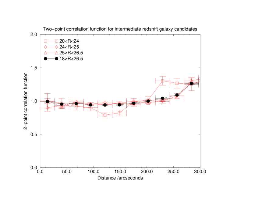
Figure 18: Two–point correlation function for the intermediate redshift candidates

Figure 21: $U-G$ vs $G-R$ colour–colour graph for PC1643+4631 showing the high–redshift selection criteria for all objects with $R<25.5$ and detections in $G$ of at least 2–$\sigma$. Dots denote detections in $U$, $G$ & $R$. Triangles denote 1–$\sigma$ lower limits in $U-G$. The crosses are stars taken from the Gunn & Stryker database, and the dot–dash lines is the bound for selecting the high redshift candidates. The tracks on this graph are for model galaxies derived using the Bruzual & Charlot 1996 distribution, as in Figure 17.

Figure 22: $R$–magnitude distribution for the high–redshift galaxy candidates

Figure 23: Spatial distribution of the high–redshift candidates, as determined using the colour criteria given in section 8.2. The dashed ellipse shows the $1\sigma$ limits of the position of the centre of the S-Z decrement.

The dotted line plotted here is the power–law $A_{\omega}\theta^{-\beta}$ with $A_{\omega}=2\textrm{arcsec}^{\beta}$ and $\beta=0.9$.

Figure 26: SEDs for the 18 objects with $R-K>3$

Figure 28: Colour–colour plot of the $R-K>3$ candidates. Circles denote detections in $U,G\ \&\ R$ and triangles are marked for all objects with $U>1\sigma$. All objects are well detected in $R$ ($R>>5\sigma$). The radii of the circles indicate the brightness – smaller implies fainter. The tracks are the evolutionary tracks as in Figure 17 and crosses are stars taken from the Gunn & Stryker 1983 database.

Figure 29: Sky positions of the $R-K>3$ candidates. The dashed ellipse shows the $1\sigma$ limits of the position of the centre of the S-Z decrement. Note that the sky coverage in $K$, indicated by the dashed boxes, covers only part of the field.

References

- [Bertin and Arnouts, 1996] Bertin, E. and Arnouts, S. (1996). SExtractor: Software for source extraction. Astronomy and Astrophysics Supplement Series, 117:393–404.
- [Brainerd and Smail, 1998] Brainerd, T. G. and Smail, I. (1998). A Constant Clustering Amplitude for Faint Galaxies? ApJ, 494:L137–+.
- [Broadhurst et al., 1995] Broadhurst, T. J., Taylor, A. N., and Peacock, J. A. (1995). Mapping cluster mass distributions via gravitational lensing of background galaxies. ApJ, 438:49–61.
- [Bruzual and Charlot, 1993] Bruzual, G. A. and Charlot, S. (1993). Spectral evolution of stellar populations using isochrone synthesis. ApJ, 405:538–553.
- [Casertano et al., 1995] Casertano, S., Ratnatunga, K. U., Griffiths, R. E., Im, M., Neuschaefer, L. W., Ostrander, E. J., and Windhorst, R. A. (1995). Structural parameters of faint galaxies from prerefurbishment Hubble Space Telescope Medium Deep Survey Observations. ApJ, 453:599+.
- [Coleman et al., 1980] Coleman, G. D., Wu, C. C., and Weedman, D. W. (1980). Colors and magnitudes predicted for high redshift galaxies. ApJS, 43:393–416.
- [Cowie and Hu, 1998] Cowie, L. L. and Hu, E. M. (1998). High-z Lyman-alpha Emitters. I. A Blank-Field Search for Objects Near Redshift z=3.4 in and around the Hubble Deep Field and the Hawaii Deep Field SSA22. AJ. In press.
- [Driver et al., 1994] Driver, S. P., Phillipps, S., Davies, J. I., Morgan, I., and Disney, M. J. (1994). Multicolour faint galaxy number counts with the hitchhiker parallel CCD camera. MNRAS, 266:155+.
- [Driver et al., 1995] Driver, S. P., Windhorst, R. A., Ostrander, E. J., Keel, W. C., Griffiths, R. E., and Ratnatunga, K. U. (1995). The morphological mix of field galaxies to m I = 24.25 mag (bJ approximately 26 mag) from a Deep Hubble Space Telescope WFPC2 image. ApJ, 449:L23–+.
- [Frayer et al., 1994] Frayer, D. T., Brown, R. L., and Vanden Bout, P. A. (1994). Co emission from the z = 3.137 damped Ly-alpha system toward PC 1643+4631A. ApJ, 433:L5–L8.
- [Giavalisco et al., 1998] Giavalisco, M., Steidel, C. C., Adelberger, K. L., Dickinson, M. E., Pettini, M., and Kellogg, M. (1998). The Angular Clustering of Lyman-Break Galaxies at Redshift z=3. AJ. In press.
- [Glazebrook et al., 1995] Glazebrook, K., Ellis, R., Santiago, B., and Griffiths, R. (1995). The morphological identification of the rapidly evolving population of faint galaxies. MNRAS, 275:L19–L22.
- [Graham and Dey, 1996] Graham, J. R. and Dey, A. (1996). The redshift of an Extremely Red Object and the nature of the very red galaxy population. ApJ, 471:720+.
- [Gunn and Stryker, 1983] Gunn, J. E. and Stryker, L. L. (1983). Stellar spectrophotometric atlas, wavelengths from 3130 to 10800 å. ApJS, 52:121–153.
- [Hall and Mackay, 1984] Hall, P. and Mackay, C. D. (1984). Faint galaxy number-magnitude counts at high galactic latitude. I. MNRAS, 210:979–992.
- [Hawkins et al., 1997] Hawkins, M. R. S., Clements, D., Fried, J. W., Heavens, A. F., Veron, P., Minty, E. M., and Van Der Werf, P. (1997). The double quasar Q2138-431: lensing by a dark galaxy? MNRAS, 291:811–818.
- [Hogg et al., 1997] Hogg, D. W., Pahre, M. A., McCarthy, J. K., Cohen, J. G., Blandford, R., Smail, I., and Soifer, B. T. (1997). Counts and colours of faint galaxies in the U and R bands. MNRAS, 288:404–410.
- [Hu, 1998] Hu, E. M. (1998). Pushing back studies of Galaxies toward the dark ages: High-Redshift Lyman alpha Emission-Line Galaxies in the field. astroph-9801170. preprint.
- [Hu and Ridgway, 1994] Hu, E. M. and Ridgway, S. E. (1994). Two extremely red galaxies. AJ, 107:1303–1306.
- [Jarvis and Tyson, 1981] Jarvis, J. F. and Tyson, J. A. (1981). FOCAS - Faint Object Classification and Analysis System. AJ, 86:476–495.
- [Jones et al., 1997] Jones, M. E., Saunders, R., Baker, J. C., Cotter, G., Edge, A., Grainge, K., Haynes, T., Lasenby, A., Pooley, G., and Rottgering, H. (1997). Detection of a Cosmic Microwave Background Decrement toward the z = 3.8 quasar pair PC 1643+4631A,B. ApJ, 479:L1–+.
- [Keeton and Kochanek, 1998] Keeton, C. R. and Kochanek, C. S. (1998). Gravitational lensing by spiral galaxies. ApJ, 495:157+.
- [Koo et al., 1986] Koo, D. C., Kron, R. G., Nanni, D., Trevese, D., and Vignato, A. (1986). A multicolor photometric catalog of galaxies and stars in the field of the rich cluster II ZW 1305.4 + 2941 at z = 0.24. AJ, 91:478–493.
- [Le Fevre et al., 1995] Le Fevre, O., Crampton, D., Lilly, S. J., Hammer, F., and Tresse, L. (1995). The Canada-France Redshift Survey. II. Spectroscopic program: Data for the 0000-00 and 1000+25 fields. ApJ, 455:60+.
- [Luppino and Kaiser, 1997] Luppino, G. A. and Kaiser, N. (1997). Detection of weak lensing by a cluster of galaxies at z = 0.83. ApJ, 475:20+.
- [Metcalfe et al., 1996] Metcalfe, N., Shanks, T., Campos, A., Fong, R., and Gardner, J. P. (1996). Galaxy formation at high redshifts. Nature, 383:236+.
- [Oke and Gunn, 1983] Oke, J. B. and Gunn, J. E. (1983). Secondary standard stars for absolute spectrophotometry. ApJ, 266:713–717.
- [Pettini et al., 1997] Pettini, M., Steidel, C. C., Adelberger, K., Kellogg, M., Dickinson, M., and Giavalisco, M. (1997). The Discovery of Primeval Galaxies and the Epoch of Galaxy Formation. In Shull, J., Woodward, C., and Thronson, H., editors, Origins, ASP Conference Series.
- [Saunders et al., 1997] Saunders, R., Baker, J. C., Bremer, M. N., Bunker, A. J., Cotter, G., Eales, S., Grainge, K., Haynes, T., Jones, M. E., Lacy, M., Pooley, G., and Rawlings, S. (1997). Optical and infrared investigation toward the z = 3.8 quasar pair PC 1643+4631A, B. ApJ, 479:L5–+.
- [Schechter et al., 1998] Schechter, P. L., Gregg, M. D., Becker, R. H., Helfand, D. J., and White, R. L. (1998). The first FIRST gravitationally lensed quasar: FBQ 0951+2635. Submitted to AJ. Preprint astro-ph/9710120.
- [Schneider et al., 1994] Schneider, D. P., Schmidt, M., and Gunn, J. E. (1994). Spectroscopic CCD surveys for quasars at large redshift. 3: The Palomar Transit Grism Survey catalog. AJ, 107:1245–1269.
- [Smail et al., 1995] Smail, I., Hogg, D. W., Yan, L., and Cohen, J. G. (1995). Deep optical galaxy counts with the Keck telescope. ApJ, 449:L105–+.
- [Songaila et al., 1990] Songaila, A., Cowie, L. L., and Lilly, S. J. (1990). Galaxy formation and the origin of the ionizing flux at large redshift. ApJ, 348:371–377.
- [Steidel et al., 1998] Steidel, C. C., Adelberger, K. L., Dickinson, M., Giavalisco, M., Pettini, M., and Kellogg, M. (1998). A large structure of galaxies at redshift z approximately 3 and its cosmological implications. ApJ, 492:428+.
- [Steidel et al., 1996] Steidel, C. C., Giavalisco, M., Pettini, M., Dickinson, M., and Adelberger, K. L. (1996). Spectroscopic confirmation of a population of normal star-forming galaxies at redshifts z 3. ApJ, 462:L17–+.
- [Steidel and Hamilton, 1993] Steidel, C. C. and Hamilton, D. (1993). Deep imaging of high redshift QSO fields below the Lyman limit. II - Number counts and colors of field galaxies. AJ, 105:2017–2030.
- [Surdej et al., 1997] Surdej, J., Claeskens, J. F., Remy, M., Refsdal, S., Pirenne, B., Prieto, A., and Vanderriest, C. (1997). HST confirmation of the lensed quasar J03.13. A&A, 327:L1–L4.
- [Thompson et al., 1995] Thompson, D., Djorgovski, S., and Trauger, J. (1995). A narrow band imaging survey for primeval galaxies. AJ, 110:963+.
- [Tody, 1993] Tody, D. (1993). IRAF in the nineties. Astronomical Data Analysis Software and Systems II, A.S.P. Conference Series, Vol. 52, 1993, R. J. Hanisch, R. J. V. Brissenden, and Jeannette Barnes, eds., p. 173., 2:173+.
- [Tyson, 1988] Tyson, J. A. (1988). Deep CCD survey - Galaxy luminosity and color evolution. AJ, 96:1–23.
- [van Kampen, 1997] van Kampen, E. (1997). Cluster mass estimation from lens magnification. In Large Scale Structure: tracks and traces. Potsdam, World Scientific. Preprint astro-ph/9711178.
- [Williams et al., 1996] Williams, R. E., Blacker, B., Dickinson, M., Dixon, W. V. D., Ferguson, H. C., Fruchter, A. w. S., Giavalisco, M., Gilliland, R. L., Heyer, I., Katsanis, R., Levay, Z., Lucas, R. A., McElroy, D. B., Petro, L., and Postman, M. (1996). The Hubble Deep Field: Observations, data reduction, and galaxy photometry. AJ, 112:1335+.
- [Witt et al., 1992] Witt, A. N., Thronson, Harley A., J., and Capuano, John M., J. (1992). Dust and the transfer of stellar radiation within galaxies. ApJ, 393:611–630.