Models of X-ray Photoionization in LMC X-4: Slices of a Stellar Wind

Abstract

We show that the orbital variation in the UV P Cygni lines of the X-ray binary LMC X-4 results when X-rays photoionize nearly the entire region outside of the X-ray shadow of the normal star. We fit models to Goddard High Resolution Spectrograph (GHRS) observations of N V and C IV P Cygni line profiles. Analytic methods assuming a spherically symmetric wind show that the wind velocity law is well-fit by $v\propto(1-1/r)^{\beta}$, where $\beta$ is likely $\approx 1.4-1.6$ and definitely $<2.5$. Escape probability models can fit the observed P Cygni profiles, and provide measurements of the stellar wind parameters. The fits determine $L_{x}/\dot{M}=2.6\pm 0.1\times 10^{43}$ erg s${}^{-1}\mbox{ M}_{\odot}^{-1}$ yr, where $L_{x}$ is the X-ray luminosity and $\dot{M}$ is the mass-loss rate of the star. Allowing an inhomogeneous wind improves the fits. IUE spectra show greater P Cygni absorption during the second half of the orbit than during the first. We discuss possible causes of this effect.

1 Introduction

Theorists have made considerable progress in explaining the stationary properties of OB star winds, and there is now a consensus that the winds are accelerated through resonance line scattering of the stellar continuum (Lucy & Solomon 1970; Castor, Abbott, & Klein 1975). The spectral lines predicted by detailed models match observations for a wide variety of ionization species (Pauldrach 1987), and for stars across a range of metallicity and evolutionary status (Kudritzki, Pauldrach, & Puls, 1987; Pauldrach et al. 1988).

However, it has become clear that real stellar winds are time-variable and contain inhomogeneities which, although expected on theoretical grounds, are difficult for the theory to treat properly. There is independent evidence for these inhomogeneities from the black absorption troughs (Lucy 1982a) and variable “discrete absorption features” seen in wind-formed P Cygni lines (Massa et al. 1995), in the X-ray emission from OB stars (Harnden et al. 1979; Seward et al. 1979; Corcoran et al. 1994), and from polarimetric observations (Brown et al. 1995), IR observations (Abbott, Telesco, & Wolff 1984) and radio observations (Bieging, Abbott, & Churchwell 1989). Theoretically, the scattering mechanism thought to be responsible for the acceleration of the wind should be unstable, leading to shocks (MacGregor, Hartmann, & Raymond 1979; Abbott 1980; Lucy & White 1980; Owocki & Rybicki 1984). Although these instabilities have been modelled numerically, the models encounter nonlinearities (Owocki, Castor, & Rybicki 1988).

The unknown nature of the wind inhomogeneities has hindered attempts to infer from observations such properties of stellar winds as the mass-loss rates, which are critical for understanding massive star evolution. The observations are, in essence, averages over the entire nonuniform and time-variable wind, and the unknown weighting of these averages prevents us from knowing the magnitude of the total mass outflow. Overcoming these difficulties is a major goal of current studies of hot stellar atmospheres.

When the OB star has an accreting compact companion, X-rays from the compact object can be used as a probe to derive parameters of the undisturbed wind, such as its mass-loss rate, expansion velocity, and radial velocity law. In the “Hatchett-McCray effect” (Hatchett & McCray 1977; McCray et al. 1984), the X-rays remove the ion responsible for a P Cygni line from a portion of the wind, resulting in orbital variations of P Cygni profiles. This effect has been observed in several High Mass X-ray Binaries (HMXB; Dupree et al. 1980; Hammerschlag-Hensberge et al. 1980; van der Klis, et al. 1982; Kallman & White 1982; Haberl, White & Kallman 1989). Analysis of the velocities over which the P Cygni lines vary has suggested that in some cases, the stellar wind radial velocity dependence can be nonmonotonic (Kaper, Hammerschlag-Hensberge, & van Loon 1993). Whether this is intrinsic to the OB star wind or is a result of the interaction with the compact object is not known.

LMC X-4 shows a more pronounced Hatchett-McCray effect than any other X-ray binary. The UV P Cygni lines of N V at 1240Å appear strong in low-resolution IUE spectra at $\phi=0$, but nearly disappear at $\phi=0.5$ (van der Klis et al. 1982). The equivalent width of the N V absorption varies by more than 100% throughout the orbit, suggesting that the X-ray source may remove N V from the entire region of the wind outside of the X-ray shadow of the normal star.

If the X-ray ionization of the wind is indeed this thorough, then the change in the P Cygni profile between two closely spaced orbital phases is largely the result of the X-ray shadow of the primary advancing through a thin “slice” of the stellar wind. Thus models of the changing P Cygni profiles should be sensitive to a region of the wind that is small in spatial extent. Vrtilek et al. (1997, Paper I) obtained high-resolution spectra of the N V lines (and the C IV $\lambda\lambda\,1548,\,1550$ lines, which show weaker variability) with the Goddard High Resolution Spectrograph (GHRS) aboard the Hubble Space Telescope. These spectra, unlike the earlier IUE spectra, provide a high enough resolution and signal to noise ratio to allow us to examine the detailed velocity structure of the P Cygni lines over closely spaced intervals of the binary orbit.

LMC X-4 consists of a main-sequence O star (variously classified as O7–9 III–V) of about $15\mbox{ M}_{\odot}$ and a $\approx 1.4\mbox{ M}_{\odot}$ neutron star with a spin period of 13.5 seconds (Kelley et al. 1983). Pulse delays from the neutron star have established the projected semimajor axis of the orbit precisely as 26 light seconds. The 1.4 day orbital period is also seen in X-ray eclipses (Li, Rappaport, & Epstein 1978) and modulations of the optical brightness (Heemskerk & van Paradijs 1989). The X-ray spectrum in the normal state is hard (photon power-index $\alpha\approx 0.8$) with little absorption of the soft X-rays (Woo et al. 1996 give $N_{\rm H}=1.14\pm 0.005\times 10^{21}$ cm^-2). The total quiescent X-ray luminosity is $\sim 10^{38}$ erg s^-1, near the Eddington limit for a $1.4\mbox{ M}_{\odot}$ neutron star.

X-ray flares, in which the pulse-averaged X-ray luminosity can exceed 10³⁹ erg s^-1, occur with a frequency of about once a day (Kelley et al. 1983; Pietsch et al. 1985; Levine et al. 1991). These flares have been interpreted as dense blobs of wind material crashing down on the surface of the neutron star (White, Kallman, & Swank 1983; Haberl, White, & Kallman 1989). It is an open question whether these blobs represent the natural state of the stellar wind, or are produced by interactions between the X-ray source and an unperturbed stellar wind. An accreting compact object embedded in a stellar wind can affect the wind through the heating, ionization, and radiation pressure of its X-ray emission, and through its gravity. Numerical simulations (Blondin et al. 1990, 1991) of the modifications of the stellar wind by the compact object show that the wind can form accretion wakes and disk-like structures (even in systems which are not thought to have substantial mass-transfer through Roche lobe overflow). Thus an investigation of instabilities in the wind of LMC X-4 also bears on the cause of the X-ray flares.

We present a series of increasingly more sophisticated models of the P Cygni lines in LMC X-4, as observed with the GHRS and reported in Paper I. In §2, we compare the N V and C IV P Cygni lines to those of isolated OB stars and to those of other massive X-ray binaries. We make inferences from analytic and approximate models to the P Cygni line variations in §3. Then we attempt more detailed models in §4, and derive best-fit parameters for the wind and X-ray luminosity.

We note that this is the first detailed fit of P Cygni lines that has been attempted for a HMXB. The sophistication of the models that we present is justified by the high quality of the data on this system that should be obtained in the near future.

2 Comparison spectra

In this section, we compare the UV line profiles of LMC X-4 with the line profiles of similar stars.

2.1 Other X-ray binaries

The strength of the orbital variation in P Cygni lines (the Hatchett-McCray effect) differs among the HMXB. Figure 1 compares the N V lines at two orbital phases with the corresponding features in 4U1700-37 and Vela X-1 (the latter two objects were observed with IUE at high spectral resolution in the echelle mode). The optical companion of 4U1700-37 is very massive ($\sim 50\mbox{ M}_{\odot}$) and hot (spectral type O6.5 with effective temperature 42,000K; Kaper et al. 1993). In this system the N V resonance line is saturated and shows little or no variation over orbital phase; this saturation is caused by the very strong stellar wind produced by the extremely massive and hot companion. The companion of Vela X-1 has a lower mass (23$\mbox{ M}_{\odot}$) and is considerably cooler (spectral type B0.5 with an effective temperature of 25,000K; Kaper et al. 1993). The wind in LMC X-4 is expected to be weaker than in Vela X-1 and 4U1700-37, as the optical companion is not a supergiant. As the abundances of metals are lower in the LMC than in the Galaxy, lower mass-loss rates for a given spectral type are expected. The low abundances will also make the N V lines less saturated and the effects of X-ray ionization more visible. The X-ray luminosity of LMC X-4 is the highest of the three systems. As a result of these considerations, it is not surprising that the effects of X-ray ionization on the N V lines are strongest in LMC X-4. For all three systems the C IV resonance lines show little orbital variation during the phases observed.

2.2 Photospheric lines at $\phi\sim 0.5$

The effects of the X-ray photoionization on the blueshifted P Cygni absorption are greatest for LMC X-4 near $\phi=0.5$. The observed N V line profiles still show residual absorption at $\phi=0.42$. Paper I interpreted this absorption to be the photospheric N V doublet, which is masked by the wind absorption during X-ray eclipse. If this interpretation is correct, the width of the absorption is determined by the rotation of the normal star, not the wind expansion velocity. Alternately, at the base of the wind where the expansion velocity is low, the wind may be dense enough that N V can still exist even in the presence of X-ray illumination.

Nearly all early-type stars whose N V photospheric absorption lines could be usefully compared with those of LMC X-4 also have strong wind absorption. The O9 IV star $\mu$Col (HD 38666) seems to be a promising candidate for comparison, as its N V line has negligible red-shifted emission, and the blue-shifted absorption is confined to features near the rest wavelength.

Although this is the best candidate for the intrinsic N V photospheric absorption spectrum that we were able to obtain, Wollaert, Lamers, & de Jager (1988) suggest that the N V and C IV lines in this star are wind-formed because they are asymmetric. We have compared IUE and HST spectra of $\mu$Col with our spectra of LMC X-4, and although the detailed fit is poor (Figure 2a), the strength of the absorption in $\mu$Col is comparable to the absorption in LMC X-4 at $\phi=0.4$. This provides qualified support that the photospheric N V lines of subgiant O stars can be comparable to the lines we see in LMC X-4.

We also compare the LMC X-4 spectra with the optical absorption lines which Hutchings et al. (1978) concluded were photospheric. Hutchings et al. found that the optical lines were consistent with an orbital velocity of $50-60$ km s^-1 and a systemic velocity of $\approx 280$ km s^-1. They measured the width of the optical lines to be $\sim 170$ km s^-1, which would be expected if the primary rotates with a period twice as long as the binary orbit. We find a good fit to the N V absorption profile using Gaussians with width (approximately equal to $v\sin i$ width) 170 km s^-1 and optical depths $\tau_{\rm b}=0.6$ and $\tau_{\rm r}=0.3$ in the blue and red components (Figure 2b).

While the N V absorption velocity agrees with both the optical absorption line velocity found by Hutchings et al. and with the systemic velocity of the LMC (Bomans et al. 1996), the cross-over between absorption and emission occurs at relative red-shifts of $100-200$ km s^-1. This may suggest that LMC X-4 has a red-shift relative to the LMC and that the “photospheric” absorption is actually blue-shifted P Cygni absorption.

In the absence of a clear means of separating the wind and photospheric absorption, we will allow, in the more detailed analysis that follows, the strength of a photospheric absorption line to be an adjustable free parameter. We note that Groenewegen & Lamers (1989) fit P Cygni lines observed with IUE, and that for the stars HD 24912, 36861, 47839, and 101413 (with spectral types O7.5 III,O8 III, O7 V, and O8 V respectively), the best-fit values of $\tau_{\rm r}$ for N V are 0.0, 0.4, 0.3, and 0.3 respectively.

3 Simple Models

In the discussion that follows, we assume that the orbital variation of the N V P Cygni lines is caused principally by the Hatchett-McCray effect, that is, through the photoionization of the stellar wind by the X-ray source. There do not appear to be any variable Raman-scattered emission lines which Kaper et al. (1993) suggested cause an orbital variability in the X-ray binary 4U 1700-37.

3.1 Equivalent width variations (IUE and HST observations)

Following van der Klis et al. (1982), we examine the orbital variation of the equivalent width of N V in LMC X-4 using a simple numeric model. Hatchett & McCray (1977) showed that the X-ray ionized zones could be approximated as surfaces of constant $q$, where each point in the wind has a value of $q$ given by

$$\frac{L_{\rm x}}{n_{\rm x}D^{2}}q=\xi.$$ (1)

Here, $L_{\rm x}$ is the X-ray luminosity, $n_{\rm x}$ is the electron density at the radius of the X-ray source ($D=1.77$ stellar radii in the case of LMC X-4), and $\xi$ is the ionization parameter $\xi\equiv L_{\rm x}/n_{\rm e}r_{\rm x}^{2}$, where $n_{\rm e}$ is the electron density at the given point, and $r_{\rm x}$ is the distance from that point to the X-ray source. Given a constant mass-loss rate $\dot{M}$ for the wind, $n_{\rm e}$ can be found from mass conservation:

$$n_{\rm e}=1.2\frac{\dot{M}}{4\pi r^{2}v}m_{\rm H}^{-1}.$$ (2)

We illustrate these parameters in Figure 3.

For large values of $q$, the surfaces of constant ionization are spheres surrounding the X-ray source, while for $q<1$, the surfaces are open. Where the surfaces extend into the primary’s X-ray shadow, a conical shape must be used instead of the constant $q$ surface. We model the absorption line variation using the velocity law $v\propto(1-1/x)$, where $x$ is the wind radial distance in units of the stellar radius. According to van der Klis et al. the results are not sensitive to the velocity law assumed. We account for the orbital inclination $i$ ($i=66.2^{+2.5}_{-2.8}\arcdeg$, Pietsch et al. 1985) by using a corrected orbital phase $\phi^{\prime}$ such that $\cos 2\pi\phi^{\prime}=\cos 2\pi\phi\sin i$. To model the orbital variation of equivalent width, we used the best-fit escape probability model we describe in §4.1, except that the only X-ray ionization occurs within the zone bounded by $q$, which is completely ionized.

We measured the equivalent width of N V, C IV, and Si IV for all the IUE observations of LMC X-4 (using the Final Archive version of the data, which has been processed by NEWSIPS, the NEW Spectral Image Processing System, de la Pena et al. 1994). We used the ephemeris of Woo et al. (1996) to find the corresponding orbital phases for each spectrum. In Figure 4, we compare theoretical variations in equivalent width with those observed with IUE and the GHRS. That is, we plot

$$\Delta\equiv(W_{\lambda}-\bar{W_{\lambda}})/\bar{W_{\lambda}}$$ (3)

where $W_{\lambda}$ is the equivalent width, and $\bar{W_{\lambda}}$ is the average value of $W_{\lambda}$. Here, $W_{\lambda}$ measures only the equivalent width of the absorption, and not the P Cygni emission. As the GHRS spectra were obtained during less than a complete binary orbit, we use the average equivalent width from the IUE observations to find the per cent variation in equivalent width for the GHRS spectra as well.

The results shown in Figure 4 are consistent with $q\lesssim 1$, in which case the X-ray source photoionizes at least the entire hemisphere opposite the primary, and possibly as much as the entire wind outside of the primary’s shadow. The fit to the IUE data is better for $q=1$ ($\chi^{2}=5.5$) than for full X-ray photoionization ($\chi^{2}=11$), although the GHRS equivalent widths agree with the prediction of full ionization. We note that interstellar and photospheric absorption lines, if present, provide additional absorption components that are not expected to show strong orbital variation. If these components are present, this would naturally explain why the fractional variation in equivalent width that we see is less than that predicted by $q\ll 1$. For example, for N V, $\bar{W_{\lambda}}=2.4$Å, while $W_{\lambda}$ due to photospheric absorption was found with the GHRS to be $\approx 0.8$Å. Without consideration of the photospheric absorption, the observed variation of 1.6Å  corresponds to $\Delta=67$%. However, this corresponds to a 100% variation in the equivalent width of absorption due to the wind alone, excluding the photospheric absorption.

It is likely that Figure 4 underestimates the per cent variation of the P Cygni absorption for the C IV and Si IV lines, as X-ray should be more effective in removing these ions from the wind than removing N V from the wind. A systematic uncertainty in choosing the continuum level will have a greater effect on the fractional variation in the equivalent width of the weaker lines, such as Si IV.

In the next section, we will make the simplifying assumption that the entire region outside the conical shadow of the normal star is ionized by the X-ray source, and from this derive the radial velocity law.

3.2 The radial velocity law from the maximum velocity of absorption

The spectra obtained with the GHRS were read out at 0.5 second intervals, using its RAPID mode (Paper I). The P Cygni absorption profile was variabile on time scales shorter than the HST orbit. We interpret this as the result of the X-ray shadow of the primary crossing the cylinder subtending the face of the primary, where the blue-shifted absorption is produced. We attempt to infer the radial velocity law in the wind from this rapid P Cygni variation and a few simple assumptions.

We assume here that X-ray photoionization removes N V and C IV from the entire wind outside of the X-ray shadow of the primary. This assumption is easily shown to be reasonable, based not only on the IUE and HST equivalent width variations (§3.1) but also on the expected value of $q$. Given a mass-loss rate of 10${}^{-6}\mbox{ M}_{\odot}$ yr^-1, a velocity at the X-ray source of 600 km s^-1, and an ionization parameter $\log\xi=2.5$ at which there should be little N V present (Kallman & McCray 1982), we find $q=0.16$.

As Buff & McCray (1974) pointed out, as an X-ray source orbits a star with a strong stellar wind, the absorbing column to the X-ray source should vary in a predictable way that depends on the wind structure and the orbital inclination. If the wind is not photoionized, then the absorbing column increases near eclipse. In a companion paper (Boroson et al. 1999) we will examine the ionization in the wind from the variation in the absorbing column as seen with ASCA. Preliminary analysis supports $q\ll 1$.

We now use the geometry shown in Figure 5. The primary star is assumed to be spherical with a radius $R$. The neutron star orbits at a radius $D$. The angle between the ray connecting the neutron star to the center of the primary and a tangent to the primary’s surface is given by $\cos\theta=R/D$. Then we define three relevant distances:

$$D_{2} \equiv \frac{R}{\cos(\pi-\theta-2\pi\phi)}$$ (4)

$$D_{3} \equiv D_{2}+\frac{RD_{2}}{D\sin 2\pi\phi}+\frac{R}{\tan 2\pi\phi},$$ (5)

$$D_{4} \equiv (D_{3}^{2}+R^{2})^{1/2}.$$ (6)

We wish to compute, given $\phi$, the radius $r(\phi)$ in the wind responsible for the maximum observed velocity of absorption. Given $(r(\phi),v(\phi))$ derived from closely spaced $\phi$ when the shadow of the primary is moving across the line of sight, we can compare with the theoretical expectation of the wind acceleration velocity law. (Note that this assumes a spherically symmetric wind.)

Given a monotonic velocity law, in most situations the maximum absorption velocity will be observed to be $V(\phi)$ corresponding to a wind radial velocity $V_{\rm max}$ (Figure 5), at a distance of $D_{4}$ from the center of the primary. This is the furthest radial distance at which the wind can absorb stellar continuum and at which the X-rays from the neutron star are shadowed by the limb of the primary. Note that the wind at this point is moving obliquely so that $V(\phi)=V_{\rm max}D_{3}/D_{4}$. As $\phi$ increases from 0.1 to 0.5, the wind at $V_{\rm max}$ will move with increasing obliqueness to the line of sight. As a result, even though this point has the greatest radial distance of any point in the wind that can absorb N V, it still may not cause the absorption with the highest possible line of sight velocity, even in a monotonic wind. As a first check to see if the obliquity of the velocity vector at $V_{\rm max}$ is important, we can compare $V(\phi)$ with $V_{\rm line-of-sight}$, which can be calculated from $D_{2}$, assuming a radial velocity law.

We assume that $D/R=1.77$, which can be calculated from the mass ratio and the assumption that the primary fills its Roche lobe. (Note that we use the separation between the centers of mass of the two stars, and not the distance of the NS from the CM of the system, which is about 10% smaller.)

We determine the maximum velocity of absorption by fitting the high-velocity edge of the absorption profile with a broken line (Figure 6). The line is horizontal for the continuum blue-ward of the maximum velocity of absorption and has a nonzero slope, allowed to vary as a free parameter, at velocities less than the maximum. When the doublets do not overlap ($\phi>0.19$), we are able to obtain two maximum velocities at each phase, one for each doublet component. For the red doublet component, we do not fit a broken line in order to determine the maximum absorption velocity, as the profile is never horizontal. Instead, we find the maximum absorption velocity in the red doublet component by determining where the flux rises to the continuum level (which is determined by the broken-line fit to the blue doublet component.) The results from the red and blue doublet components do not show a systematic difference. Thus averaging maximum absorption velocities determined in each line allows us to reduce the errors in our velocity measurements.

We can apply a further refinement to the method. The observed P Cygni trough is actually a sum of the true absorption profile and blue-shifted P Cygni emission. The observed maximum absorption velocity may be shifted by the addition of the emission. Although we can not observe the blue-shifted emission profile directly (it is masked by the absorption whose profile we are trying to uncover) we can approximate it using the reflected red-shifted profile at a complementary orbital phase, assuming spherical symmetry and the Hatchett-McCray effect. The emission flux $F$ at velocity $v$ and at phase $\phi$ is given by

$$F(v,\phi)\approx F(-v,0.5-\phi).$$ (7)

For example, at $\phi=0.1$, the red-shifted emission at high velocities will be diminished as a result of photoionization; the blue-shifted emission at $\phi=0.4$ will be similarly diminished. (This symmetry is broken because the primary shadows a portion of the red-shifted emission but none of the blue-shifted emission. However, we can safely neglect this effect because the blue-shifted emission in front of the stellar disk can not have a higher velocity than the blue-shifted absorption.)

The zero-velocity for the reflection of the red-shifted emission is not completely constrained. We allow two choices: 1) that the systemic velocity of LMC X-4 is identical to that of the LMC, and 2) that the systemic velocity of LMC X-4 is 150 km s^-1 so that the turnover between red-shifted emission and blue-shifted absorption occurs near a velocity of 0.

We give the measured values of $(r(\phi),v(\phi))$ in Table 1. We consider that a reasonable $1\sigma$ error for the velocity measurements is 50 km s^-1.

As an independent check on our measurements of wind velocity, we examine the maximum velocities at which the absorption profiles vary between two orbital phases. This is the only method we can apply to the C IV$\lambda 1548$ lines, in which the P Cygni absorption can not be separated from the strong interstellar and photospheric lines by examination of the spectrum alone. The best-fit maximum velocity of the C IV line is at $910\pm 50$ km s^-1. We note that we did not observe any red-shifted P Cygni emission in C IV, so were unable to compensate for the variability in the blue-shifted emission.

The maximum velocity of the change in N V absorption between $\phi=0.111$ and $\phi=0.209$ is $1130\pm 50$ km s^-1, consistent with the measurements in Table 1. Between $\phi=0.209$ and $\phi=0.312$, the peak velocity of absorption variations is $560\pm 50$ km s^-1, consistent with the previous measurements (depending on the model of the blue-shifted emission that is subtracted). However, between $\phi=0.312$ and $\phi=0.410$, the maximum velocity of the absorption variations is $160$ km s^-1. This is lower than the velocity inferred from the line profiles alone ($\approx 320$ km s^-1 at $\phi\approx 0.312$).

As discussed in §2.2, the blueshifted absorption may have a component which is produced near the stellar photosphere, rather than in the wind. In this case, the velocity width of the line may be produced by the rotation of the star, rather than the wind expansion. We suggest that the absorption line for $\phi>0.25$ is likely to contain a large photospheric component. Thus we do not fit to the maximum absorption velocity at these phases.

We fit our measurements of $(r(\phi),v(\phi))$ to the analytic expression

$$v=v_{\infty}(1-1/x)^{\beta}+v_{0}$$ (8)

where $v_{0}$ is the systemic velocity of LMC X-4, and $x=r/R$. The best-fit values and formal errors are presented in Table 2, for 3 possibilities of organizing the data, depending on whether we subtract our model for the blue-shifted emission from the spectra and whether the velocity of the reflection point is 0 or 150 km s^-1. We find the best fit using a downhill simplex method (Nelder & Mead, 1965) and estimate errors using a Monte-Carlo bootstrap method.

We plot $(r(\phi),v(\phi))$ (measured from both doublet components) in Figure 7, along with the analytic fits. There is no evidence that the wind is nonmonotonic. All the results indicate that the wind expands more slowly than expected from the radiatively accelerated solution (which can be well-approximated with $\beta=0.8$; Pauldrach, Puls, & Kudritzki 1986). While there is a large range of $\beta$ that can fit the 3 arrangements of observing $(r(\phi),v(\phi))$ ($1.4<\beta<2.4$), the choice of $\beta=1.39\pm 0.14$ provides the lowest $\chi^{2}$ and the most reasonable systemic velocity. (However, note that turbulence in the wind could add a constant velocity to the absorption edge and could cause the data to be well-fit by a nonphysical value of the systemic velocity.) The models are also consistent with the measurements of the wind veocity from differences of successive spectra of C IV at $\phi=0.15$ and N V at $\phi=0.3$.

While a coincident stellar absorption feature at $\lambda\approx 1249$Å decreases the red-shifted emission for velocities $v\gtrsim 1000$ km s^-1, compensating for this feature in our subtraction of the blue-shifted emission would only increase slightly the value of $\beta$ that we measure.

Our fits for the stellar wind acceleration parameter $\beta$ are not sensitive to our choice of $D=1.77$; using $D=1.70$ and $D=1.84$ we find $\beta$ within $1\sigma$ of values in the first two rows of Table 2, but $\beta=2.00$ instead of $2.37\pm 0.11$ for the third row.

The effects of microturbulence in the wind on the measured maximum wind velocity should not alter the values we have found for $\beta$. For example, if the microturbulence velocity is constant, then our fits would give a different value of $v_{0}$ but the same $\beta$. If the microturbulence velocity is a constant fraction of the wind velocity, then as a rough approximation, all measured values of $v(\phi)$ will be multiplied by a constant, leading us to fit $(r(\phi),v(\phi))$ with a different value of $v_{\infty}$ but the same value of $\beta$.

In this section we have demonstrated a new method of probing the velocity field of a stellar wind. We have assumed only standard parameters of the stellar radius and separation, that the wind is spherically symmetric and that the X-ray source completely ionizes the wind. One drawback of the method is that only a very small portion of the available data is used, that is, only the velocity of the edge of the absorption. In the next section, we adapt the method to fit the entire absorption profile.

3.3 The Radial Velocity Law from the Absorption Line Profile

We now attempt to fit the entire absorption profile to determine the wind radial velocity law. The geometry of this method is shown in Figure 8. The X-ray shadow of the primary is conical. At distances $r\gg R$ from the center of the primary, the wind within the cylindar subtending the stellar surface has only a small oblique velocity (assuming a radial velocity field). Thus the surfaces of constant projected velocity, far from the primary, are planes perpendicular to the line of sight. The intersection between the cone of shadow and the planar isovelocity surface at a given observed velocity will most often be a parabola. This parabola bounds those portions of the stellar disk that lie behind unilluminated gas at the observed velocity, and thus are absorbed by the N V in the wind, and those portions that do not.

If we could obtain an image of the stellar disk of the primary in LMC X-4 with a narrow-band filter centered at a wavelength corresponding to a Doppler shift at the given velocity, we would see a crescent-shape bounded by the star’s disk and the parabola. As the wavelength of the filter approached the terminal velocity of the wind, the intersection of the plane and cone would bound a smaller and smaller region of the stellar surface, and would thus determine the shape of the edge of the P Cygni profile.

In general, the isovelocity surfaces will not be planes, and we will need to solve for them numerically. We can no longer simply read off the velocity corresponding to each radius from the absorption profile, as we did in §3.2. Instead, we need to assume a velocity law, find the isovelocity surfaces, find their intersection with the conical shadow, and then compute the absorption profile and compare with the observed profile.

To use the observed absorption profile, we must correct for the blue-shifted emission by subtracting the red-shifted emission at a complementary phase. Now that we consider the line profile and not merely the edge of the absorption, we must recognize the asymmetry between the red and blue-shifted emission profiles at $\phi$ and $0.5-\phi$ which is introduced by the primary’s shadow of the red-shifted emission. We correct for this by assuming that the shadowed red-shifted emission at the complementary phase is given by

$$F_{\rm shadow}(v,\phi)=-\frac{1}{2}\left(1-\frac{\sqrt{x^{2}-1}}{x}\right)F_{\rm abs}(-v,0.5-\phi)$$ (9)

where $x$ is the radial distance in the wind, normalized to the stellar radius, $F_{\rm shadow}$ is the line profile of the shadowed part of the red-shifted emission, and $F_{\rm abs}$ is the intrinsic absorption line profile. For this approximation, we have noted that the shadowed red-shifted emission at $\phi$ corresponds to the blue-shifted absorption at $0.5-\phi$, with the dilution factor needed to compare the absorption with the emission.

We also need to assume an optical depth in the wind. As a first attempt, we assume that the wind is entirely black to the continuum in the region of N V. We neglect limb and gravity darkening of the primary, and its nonspherical shape. We correct for the photospheric absorption by subtracting the profile at $\phi=0.4$, when we assume the absorption is entirely photospheric.

A fit to individual short subexposures, as in §3.2 would not be time-efficient. Instead, we fit to the blue doublet component absorption profiles at $\phi=0.1,0.2,0.3$. The fit is poor, with $\chi^{2}_{\nu}=11$ with 253 degrees of freedom, $v_{\infty}=1780\pm 10$ km s^-1, $v_{0}=110\pm 10$ km s^-1, and $\beta=4.25\pm 0.08$, which we do not consider a reasonable value. Allowing a uniform optical depth $\tau$ in the wind gives a better fit, with $\chi^{2}=2.95$, $v_{\infty}=1330\pm 30$ km s^-1, $v_{0}=72\pm 24$ km s^-1, $\beta=1.57\pm 0.04$, and $\tau=0.97\pm 0.06$. We show the results of this fit in Figure 9. This high value of $\beta$ is similar to those found in §3.2.

In the following section, we will investigate detailed numeric models of the wind, relaxing our assumption that the X-rays ionize the entire wind outside the X-ray shadow of the normal star. We do not remove the restriction that the wind velocities are spherically symmetric, as this would allow more than one point along the line of sight to be at the same projected velocity, which would require us to use more sophisticated but time-consuming techniques, such as Monte-Carlo simulation of P Cygni profiles.

4 Escape Probability Models

4.1 Methods and basic models

To model the P Cygni line variations, we apply and extend the method of McCray et al. (1984). We compute the line profiles using the Sobolev approximation and the escape probability method (Castor 1970; Castor & Lamers 1979), using a wind velocity law given by Equation 8 with $\beta=1$. The optical depth in the undisturbed wind obeys

$$\tau=T(1+\gamma)r^{-\gamma}$$ (10)

where $T$ and $\gamma$ are empirical parameters (Castor & Lamers 1979).

The optical depth of gas illuminated by the X-ray source is given by the Sobolev approximation,

$$\tau=(\pi e^{2}/mc)f\lambda_{0}n_{\rm i,j}(dv/dr)^{-1},$$ (11)

where $e$ is the electron charge, $m$ the electron mass, $\lambda_{0}$ the rest wavelength of the transition, $f$ the oscillator strength, and $n_{i,j}$ the particle density of element $i$ in ionization state $j$. From mass conservation, $n_{i,j}$ is given by

$$n_{\rm i,j}=\frac{\dot{M}}{4\pi r^{2}v}m_{\rm H}^{-1}a_{\rm i}g_{\rm i,j},$$ (12)

where $g_{i,j}$ is the fraction of element $i$ in ionization state $j$, and $a_{\rm i}$ is the fractional abundance of element $i$. Given a value of $\xi$ and the shape of the X-ray spectrum, the ion fraction $g_{i,j}$ (and thus $n_{\rm i,j}$) can be computed. For this we used the XSTAR code (Kallman & Krolik, based on Kallman & McCray 1982), which requires that the X-ray luminosity $L_{\rm x}$ be integrated over the energy range 1–1000 Ry (13.6 eV–13.6 keV). The effectiveness of X-ray photoionization depends on the X-ray spectrum; we have used a broken power-law spectrum,

$$F(E) = KE^{0.37}\qquad\mbox{for }E<25\mbox{ keV}$$ (13)

$$= KE^{-2}\qquad\mbox{for }E>25\mbox{ keV},$$ (14)

where $F(E)$ is the energy spectrum. The power-law index for $E<25$ keV was determined from simultaneous ASCA observations of the 0.4–10 keV spectrum (Paper I), while the high-energy cutoff has been observed at other times using GRANAT (Sunyaev et al. 1991). Adding a soft blackbody that contributes $\sim 10$% to the total flux (as seen in the X-ray spectrum with ASCA) has little effect on the ion fractions. We can treat the combined effect of the background ionization (due to the photospheric EUV flux or X-ray emission from shocks in the wind for example) and the X-ray ionization by

$$g_{i,j,\rm tot}=(1/g_{i,j,\rm X}+1/g_{i,j,\rm back}-1)^{-1},$$ (15)

in the case in which the wind in the absence of X-ray illumination is at least as highly ionized as the ion which causes the P Cygni line. If this is not the case, then we have

$$1/g_{i,j,\rm tot}-1=(1/g_{i,j-1,\rm X}+1/g_{i,j-1,\rm back}-2)^{-1}$$ (16)

In Equations 15 and 16, $g_{i,j,\rm X}$ and $g_{i,j,\rm back}$ are, respectively, the ion fractions with X-ray illumination (computed using XSTAR) and without (computed from equations 10, 11, and 12).

We assume that all N in the unilluminated wind is ionized to at least N V and apply Equation 15. The models of $\tau$Sco ($T\approx$30,000) by MacFarlane, Cohen, & Wang (1994) predict that the dominant ionization stage of N in the wind is N VI for wind velocities $v>0.2v_{\infty}$. In these models, the wind is ionized by X-rays, presumably caused by shocks in the wind, that have been observed by ROSAT. However, MacFarlane et al. found that their model of $\tau$Sco did not match UV observations, and that X-rays were less effective in ionizing the denser winds of hotter stars (consistent with the results of Pauldrach et al. 1994). We also tested models in which N IV was the dominant ionization stage of the unilluminated wind, and found that the best-fit parameter values were within the errors of the model we present here. The choice of Equation 15 or Equation 16 has a small effect on our results, as it affects only that portion of the wind that is illuminated by direct X-rays from the neutron star, yet is ionized so slightly that the background ionization rate is important.

We treat the overlap of doublet components using the approximation of Castor & Lamers (1979). The optical depths in the photospheric absorption lines are assumed to have Gaussian profiles. The red and blue doublet components of the photospheric lines have optical depths at line center of $\tau_{\rm b}$ and $\tau_{\rm r}=0.5\tau_{\rm b}$ (in the lines we consider, the oscillator strengths are in a 2:1 ratio).

We do not account for limb and gravity darkening of the companion or its nonspherical shape. However, we normalize the absorbed continuum (which arises in the visible face of the star) to the continuum level observed by the GHRS at each particular orbital phase, while we normalize the scattered emission (which can originate anywhere on the companion) to the average continuum level observed with the GHRS.

The free parameters of the fit are $T$, $\gamma$, $v_{\infty}$, $v_{0}$ (the systemic Doppler shift of LMC X-4), $L_{38}/\dot{M_{-6}}$ (the ratio of X-ray luminosity in 10³⁸ erg s^-1 to mass-loss rate in 10${}^{-6}\mbox{ M}_{\odot}$ yr^-1), $\dot{M_{-6}}$, and $\tau_{\rm b}$. We employ a downhill simplex method (Nelder & Mead, 1965) to find the minimum $\chi^{2}$ and then refine the solution and find errors in the parameters using the Levenberg-Marquart method (Marquardt, 1963). For all velocities, we set the error to at least 35 km s^-1, which is the resolution limit of the GHRS G160M grating. We exclude from the fit the central 1Å region around the rest wavelength of each transition, which is poorly modeled by the escape probability method.

In Table 3 we show the best-fit parameters and we display the fits to the line profiles in Figure 10.

The fits determine $L_{38}/\dot{M_{-6}}=0.26\pm 0.01$ because the ion fractions in the wind (and thus the optical depths) depend sensitively on this ratio. The fits also determine $\dot{M_{-6}}a_{\rm N}/a_{\rm N,LMC}=3.2\pm 2.3$, where $a_{\rm N,LMC}=1.8\times 10^{-5}$ is the Nitrogen abundance in the LMC, assumed to be 20% of the cosmic value. The error determined for this parameter shows that it is not effectively constrained by the fit; this is because it only affects linearly the optical depth in the portion of the wind outside of the X-ray shadow.

In general, the model successfully matchess the change in the P Cygni profiles between successive orbital phases (Figure 10, right-hand panel). However, the predicted change in the N V profiles between $\phi=0.31$ and $\phi=0.41$ is blue-shifted from the observed change. This is further evidence that the wind expands more slowly at small radii than expected from a $\beta=1$ velocity law.

4.2 Wind Inhomogeneities

We now allow the wind density to be inhomogeneous by adding two new free parameters, another mass-loss rate $Z\dot{M}$, where $Z\gg 1$, and a covering fraction $f$. In the absence of X-ray photoionization, the optical depth in the two wind components are $\tau_{1}=\tau$ (where $\tau$ is given by Equation 10) and $\tau_{2}=Z\tau$. The ionization fractions are computed for a given point in the wind that has a density determined from $\dot{M}$ and $Z\dot{M}$. For the blue-shifted absorption, a fraction $f$ of sightlines to the stellar surface encounters material with the higher density. This material has a much higher optical depth, as not only is there more of this material, but it also contains a higher fraction of N V.

Applying a downhill simplex $\chi^{2}$ minimization algorithm gives an improved $\chi^{2}_{\nu}=4.01$. The fit is improved for two reasons. First, the fit of the homogeneous wind model over-predicted the effects of X-ray ionization on the red-shifted emission (Figure 10). The inhomogenous wind model allows more N V to survive in the X-ray illuminated wind, so that more of the red-shifted emission persists. Second, the homogeneous wind model predicts too much absorption in the 1238Å line and not enough absorption in the 1242Å line at $\phi=0.12$. When an inhomogeneous wind is allowed, the strength of the absorption in the two components can be more nearly equal, as absorption from the dense wind is saturated. We compare the inhomogeneous wind models with the GHRS observations in Figure 11.

We find a “covering fraction” $f=0.33\pm 0.01$; this is the probability that a ray from the primary encounters denser material with the mass-loss rate $Z\dot{M}$. Our best-fit values are $Z=700\pm 200$ and $L_{38}/\dot{M_{-6}}=160\pm 40$. If we assume that the covering fraction is approximately the volume filling factor, then the average mass-loss rate of the wind, $\bar{\dot{M}}=(1-f)\dot{M}+fZ\dot{M}$, then leads to $L_{38}/\bar{\dot{M{-6}}}=0.7\pm 0.4$.

We note that the best-fit value for the photospheric optical depth in the blue doublet component, $\tau_{\rm b}=0.62\pm 0.02$ is higher than the values obtained for similar stars by fits to IUE data (Groenewegen & Lamers 1989).

4.3 Alternate Velocity Laws

As discussed in §3.2, the change in the maximum velocity of the P Cygni line absorption over orbital phase allows us to infer the radial velocity law in the wind, assuming only that the X-ray source ionizes the entire wind outside of the shadow of the normal star. In §4.1, we modelled the P Cygni line variations allowing the X-ray photoionization of the wind to vary but assuming a standard $\beta=1$ radial velocity law. If we allow a slowly accelerating wind with $\beta=1.6$ we can still obtain a good match with the observed line profiles, with $\chi^{2}=4.91$. In this case we find $v_{\infty}=1560\pm 35$ km s^-1, $L_{38}/\dot{M}_{-6}=0.23$ Allowing an inhomogeneous wind improves the fit to $\chi^{2}=4.59$. We conclude that while the line profiles can be adequately fit with a $\beta=1$ velocity law, a more slowly accelerating wind, inferred from simpler models, is still consistent with the data. Velocity laws with $\beta>2$ (as in some of the fits in §3.2) generally predict steeply peaked red-shifted emission (Castor & Lamers 1979); however this is difficult to rule out from the data, as photospheric absorption is probably present at low velocities.

4.4 X-ray Shadow of the Accretion Disk and Gas Stream on the Wind

The accretion disk or gas stream from the L1 point could presumably shadow regions of the stellar wind from X-ray illumination. We have made models to find signatures of these effects in the P Cygni line profiles.

LMC X-4 shows a $\approx 30$ day variation in its X-ray flux (Lang et al. 1981), usually attributed to shadowing by an accretion disk that we observe at varying orientations. To allow the disk to shadow regions of the wind from the X-rays, we make the simple assumption that it is flat but inclined to the orbital plane. Howarth & Wilson (1983) used a similar geometry to model the optical variability of the Hercules X-1 system, which shows a similar 35 day X-ray period. We allow as free parameters the angular half-thickness of the disk, its tilt from the orbital plane, and its “precessional” phase within the 30-day cycle. Fixing the 30-day phase to be the at the X-ray maximum (as suggested by observations with the All Sky Monitor on the Rossi X-ray Timing Explorer, Paper I), we perform a $\chi^{2}$ fit and find a disk half-thickness of $6.9\pm 0.3\arcdeg$ and a disk tilt of $31\pm 2\arcdeg$ from the orbital plane, for a reduced $\chi^{2}=4.62$.

To simulate the shadow caused by the gas stream from the L1 point, we have assumed that the stream emerges at an angle of $22.5\arcdeg$ from the line to the neutron star (Lubow & Shu 1975). The stream blocks the X-rays from a uniform half-thickness $\rho$ in elevation from the orbital plane (as seen from the X-ray source) and at angles $<\eta$ from the line to the L1 point along the orbital plane; $\rho$ and $\eta$ are free parameters of the fit. The fit gives $\chi^{2}=4.04$, with $\rho=33\pm 2\arcdeg$ and $\eta=90\pm 3\arcdeg$. The values for the other free parameters similar to those found in §4.1.

The reason that the gas stream shadow improves the P Cygni profile fits is that at $\phi=0.1-0.4$, the stream shadows the receding wind, increasing the red-shifted emission, which our basic model of §4.1 underpredicts. Allowing an inhomogeneous wind as in §4.2 improves the fit for the same reason. It is possible that both effects are combined, and future observations will be needed to disentagle them.

4.5 C IV Lines

The C IV $\lambda\lambda\,1548,\,1550$ lines did not show as much variability with the GHRS as the N V lines, although we did not observe the lines before $\phi=0.16$. Most of the absorption in these lines is probably either interstellar or photospheric (Vrtilek et al. 1997). Nevertheless, as a check on our models of the N V lines, we also performed fits to the C IV $\lambda\lambda\,1548,\,1550$ lines. We fix the parameters found in §4.1, except for $T$, $\gamma$, and $\tau_{\rm b}$, which are free parameters defining the optical depth of C IV in the wind and photosphere. We added fixed Gaussian interstellar C IV $\lambda\lambda\,1548,\,1550$ absorption lines to the profiles.

The result of our model, shown in Figure 12, does not match the line profiles in detail ($\chi^{2}=11.3$). It is possible that the fit is poor because there are photospheric lines in the vicinity of 1550Å due to ions other than C IV. A systemic velocity closer to 0 might bring the photospheric lines into closer agreement with the data. In both the observed profile and in the model, red-shifted emission is not prominent. The fitted value of $\gamma=7.9\pm 0.8$ implies that C IV in the undisturbed wind is confined to $x<2$, so that much of the red-shifted C IV emission could be occulted by the primary. If we fit the line profiles with models with higher values of $\beta$, then $\gamma$ is reduced, but our fits never gave $\gamma<4.5$ for $\beta<2.4$ (the upper limit found in §3.2).

We compare our values of $\gamma$ with the optical depth law found for C IV $\lambda\lambda\,1548,\,1550$ by Groenewegen & Lamers (1989) by fitting the C IV $\lambda\lambda\,1548,\,1550$ P Cygni lines of similar stars observed with IUE. They parameterize the optical depth in the stellar wind by

$$\tau\sim(v/v_{\infty})^{\alpha_{1}}[1-(v/v_{\infty})^{1/\beta}]^{\alpha_{2}}$$ (17)

where $\alpha_{2}=\gamma$ for $\alpha_{1}=0$ and $\beta=1$. For HD 36861 (spectral type O8 III) Groenewegen & Lamers find $\alpha_{1}=1.5\pm 0.2$ and $\alpha_{2}=3.1\pm 0.5$, which is inconsistent with $\gamma>3.1$. For HD 101413, they find $\alpha_{1}=-0.8\pm 0.3$ and $\alpha_{2}=1.6\pm 0.4$. These values imply a sharply peaked concentration of C IV towards the stellar surface, but do not fit our data as well as $\gamma\mathrel{>\kern-10.00002pt\lower 3.87495pt\hbox{$\sim$}}5$.

We have no compelling alternate explanation for our high value of $\gamma$. However, the C IV $\lambda\lambda\,1548,\,1550$ lines in LMC X-4 that we observed were weak and were dominated by photospheric absorption. Further observations at phases when C IV $\lambda\lambda\,1548,\,1550$ is more prominent are needed to test our conclusion that this ion is concentrated near the stellar surface.

4.6 Fits using the SEI method

It has been shown (Lamers et al. 1987) that inaccuracies resulting from the escape probability method can be reduced by computing the radiative transfer integral exactly along the line of sight while continuing to use the source function given by the Sobolev approximation. This is called the SEI (Sobolev with Exact Integration) method. The method can be used to simulate the effects of local turbulence within the wind, and using the method of Olson (1982), the effects of overlapping doublets can be computed precisely.

We have implemented a program that uses the SEI method to predict the P Cygni line profiles from a wind ionized by an embedded X-ray source. The details of the wind ionization are identical to those given by Equations 11 through 16. We find that in our analysis of LMC X-4, the approximation we have made for the doublet overlap gives results very close to those given by Olson’s method and the SEI method. This may result from the small amount of the doublet overlap in the N V $\lambda\lambda\,1238.8,\,1242.8$ lines, given a separation of 960 km s^-1 between the doublet components and a wind terminal velocity of 1350 km s^-1. Using a turbulent velocity $v_{\rm t}$ that is constant throughout the wind, we find that the line profiles are best fit with $v_{\rm t}<200$ km s^-1.

The SEI method also confirms the results of the escape probability model for the C IV $\lambda\lambda\,1548,\,1550$ lines, as reported in §4.5. Although the separation of the C IV $\lambda\lambda\,1548,\,1550$ lines is only 500 km s^-1, we suggest that the doublet overlap was not severe during our observations because much of the wind at high velocity had already been ionized, and C IV is concentrated near the primary’s surface, at low wind velocities.

5 Discussion

We have demonstrated a new method for inferring the radial velocity profile in a stellar wind. The wind radial velocity law for LMC X-4 can be fit with $\beta\approx 1.4-1.6$, and $\beta<2.5$. This differs from the expected value of $\beta=0.8$, but the wind in the LMC X-4 system is likely to deviate from that of an isolated O star. Assumptions of the method, that the wind is spherically symmetric, for example, will need to be revised in light of further observations that cover the entire orbital period.

Unfortunately, we did not observe the UV spectrum during the X-ray eclipse when the X-ray ionization of the blueshifted absorption should be minimal, and so our inference of the wind terminal velocity is model-dependent. Observations with STIS and the Far Ultraviolet Spectroscopic Explorer (FUSE) during eclipse may distinguish between our alternate models. The wind terminal velocity we have inferred from our $\beta=1$ escape probability method, $v_{\infty}=1350\pm 35$ km s^-1, is lower than the terminal velocities measured for similar stars by Lamers, Snow, & Lindholm (1995). Their stars # 33,37,38,39, and 44 are all near the 35,000 K temperature of LMC X-4, but have $v_{\infty}=1500-2200$ km s^-1. However, stars in the LMC are known to have terminal velocities $\approx 20$% lower than their galactic counterparts (Garmany & Conti 1985).

We note from the IUE data shown in Figure 4 that the P Cygni line absorption at orbital phases $\phi>0.5$ is greater than that at $\phi<0.5$. X-ray absorption dips are frequently seen at $\phi\sim 0.8$, possibly indicative of dense gas in a trailing gas stream or accretion wake. However, it may be difficult for models to reproduce an accretion wake that occults a large fraction of the primary at orbital phases as late as 0.9. Another possible explanation is that a photoionization wake is present (Fransson & Fabian 1980, Blondin et al. 1991). Such a wake results when the expanding wind that has not been exposed to X-rays encounters slower photoionized gas. While a strong photoionization wake is expected for $q\ll 1$, the presence of Roche lobe overflow and a photoionization wake have been found to be mutually exclusive in some simulations (Blondin et al. 1991). A further possibility is that at $\phi\sim 0.6-0.9$ the wind in the cylindar subtending the primary’s disk is shielded from ionization by the trailing gas stream. A simple prediction of this scenario is that there should be more flux in the red-shifted emission at $\phi=0.25$ than at $\phi=0.75$. If the primary star does indeed rotate at half the corotation velocity (Hutchings et al. 1978) then the gas stream may trail the neutron star by more than the 22.5$\arcdeg$ predicted by Lubow & Shu (1975).

We have fit the changing P Cygni line profiles using an escape probability method, assuming a radial, spherically symmetric stellar wind. However, we note that the Hatchett-McCray effect is most sensitive to the region between the $q=1$ surface and the conical shadow of the primary. Outside of this region, the wind should be entirely ionized for likely values of $\dot{M}$ and $L_{\rm x}$. The region of the wind that our method is sensitive to is illuminated by X-rays, and its dynamics may be affected as a result (Blondin et al. 1990). Structure associated with the distortion of the primary, such as the gas stream and a wind-compressed disk (Bjorkman 1994), may be also be important in this region.

We have inferred $L_{38}/\dot{M}_{-6}=0.26\pm 0.01$ from our escape probability P Cygni line models. Our simultaneous ASCA observations found a 2–10 keV flux of $2.9\times 10^{-10}$ erg s^-1 cm^-2, which given a distance to the LMC of 50 kpc implies $L_{38}=0.9$ and $\dot{M}_{-6}\approx 3$ (our inhomogeneous wind model of §4.2 would imply $\dot{M}_{-6}\approx 1$). There is some uncertainty in applying $L_{38}=0.9$, as the isotropic X-ray spectrum and luminosity may differ from that observed by ASCA. Nevertheless, the derived $\dot{M}$ is an order of magnitude larger than that reported by Woo et al. (1995), who used the strength of scattered X-rays to find $\dot{M}/v_{\infty}=10^{-10}\mbox{ M}_{\odot}$ yr^-1 (km s^-1)^-1, implying for our best-fit value of $v_{\infty}=1350\pm 35$ km s^-1 that $\dot{M}_{-6}=0.14$. Our result for $\dot{M}$ is on the order of the single-scattering limit given by the momentum transfer from the radiation pressure of the primary; $\dot{M}<L_{\rm opt}/v_{\infty}c$, where the optical luminosity of the primary $L_{\rm opt}\sim 5\times 10^{38}$ erg s^-1 (Heemskerk & van Paradijs 1989) implies that $\dot{M}<2\times 10^{-6}\mbox{ M}_{\odot}$ yr^-1. However, if the wind is accelerated by scattering of overlapping lines, one can have $\dot{M}=2-5L_{\rm opt}/v_{\infty}c$ (Friend & Castor 1982).

Combining our value of $\dot{M}_{-6}\approx 3$ with our measured wind velocity near the orbit of the neutron star (400 km s^-1) and the orbital velocity of the neutron star (440 km s^-1), we find that gravitational capture of the stellar wind (Bondi & Hoyle 1944) could power a significant portion of the observed X-rays ($L_{38}\approx 0.3$). However, we can not rule out that the low velocity and high wind density we have measured are attributable not to an isotropic wind, but to other gas in the system, such as the gas stream or a wind-compressed disk about the primary.

A comparison of the LMC X-4 N V line profiles with those of Vela X-1 and 4U1700-37.

Comparison of the N V lines in LMC X-4 observed at $\phi=0.42$ with (a) the same region in the spectrum of $\mu$Col (dot-dashed; the flux and systemic velocity have been normalized to that of LMC X-4), and (b) Gaussian lines at the systemic velocity of the LMC and with the same width as optical lines attributed to the photosphere of the primary. The vertical lines show the rest wavelenths of the N V lines.

The geometry of the Hatchett-McCray $q$ parameter. Surfaces with constant values of $q$ bound regions of the wind at different ionization levels. The primary star is represented as a circle centered at the origin, and the X-ray source is marked with an ‘X’.

Variations in the equivalent width of a) N V, b) C IV, and c) Si IV. The “*” signs mark the equivalent widths from IUE observations reported by van der Klis et al. (1982), while the “+” signs are based on the data reported in Paper I. The error bars show the $1\sigma$ error range. Also shown are theoretical models in which the ion is removed from regions of the wind with various values of the Hatchett-McCray parameter $q$.

The geometry used by a simple analytic method to infer the radial wind velocity from P Cygni line variations. The viewer is towards the bottom of the page. The circle represents the surface of the primary star and the point marked “NS” represents the neutron star. $V(\phi)$ marks the highest observed velocity of absorption. In (a) we show the situation at $\phi=0.21$ and in (b) we show $\phi=0.32$.

An example of the measurement of $V(\phi)$, the maximum velocity of absorption at a given orbital phase. We fit the edge of the observed line profile (the dotted line shows the smoothed spectrum) to a horizontal line segment for blue-shifts $V>V(\phi)$ and to a line segment with slope as a free parameter for $V<V(\phi)$. The vertical line marks the measured value of $V(\phi)$ for the 1242.8Å doublet component, determined by where the continuum reaches the same level as for the horizontal line segment.

The wind expansion velocity versus radial distance, as inferred from the P Cygni line profiles. The “*” signs mark points determined from the absorption profile. For points marked with “+” signs, a model of the blue-shifted emission as the red-shifted emission reflected about $v=150$ km s^-1 has been subtracted from the P Cygni profiles. For points marked with diamonds, the red-shifted emission was reflected about $v=0$ km s^-1. Points marked with “x” were determined from differences of spectra corrected for blue-shifted emission. The solid line shows the best fit for the diamonds for $\phi<0.25$ ($R>2$).

An illustration of a model that fits the absorption line profiles to determine the wind acceleration parameter $\beta$. The conical X-ray shadow of the primary intersects isovelocity surfaces at $v/v_{\infty}=0.2,0.4$. These intersections determine images of the primary’s surface at Doppler-shifted wavelengths corresponding to $v/v_{\infty}=0.2,0.4$. The contribution to the absorption line profile at $v/v_{\infty}=0.2,0.4$ is determined by the fraction of the primary’s surface that is not in shadow.

The best-fit model (dashed) to the N V absorption line profiles, allowing the wind acceleration parameter $\beta$ and the wind optical depth $\tau$ as free parameters, and assuming the X-rays photoionize the entire wind outside the shadow of the primary. We have subtracted a model of the blue-shifted P Cygni emission in order to fit only the blue-shifted P Cygni absorption.

The results of the best-fit model of the P Cygni line variations. The right panel shows the differences between successive orbital phases, for both the data and model.

The results of the best-fit model of the P Cygni line variations, for the inhomogeneous wind model. The right-hand panels show the differences between successive spectra.

The results of the best-fit model of the C IV P Cygni line variations.

$\phi$	$\phi^{\prime}$	$V_{\rm obs}$	$V_{\rm sub,0}$	$V_{\rm max,0}$	$D_{2}$	$D_{3}$	$D_{4}$
		(km/s)	(km/s)	(km/s)	(R⋆)	(R⋆)	(R⋆)
0.095	0.114	1270	1260	1260	8.82	17.57	17.60
0.099	0.117	1450	1390	1390	7.59	15.11	15.15
0.102	0.120	1220	1210	1210	6.66	13.24	13.27
0.106	0.123	1250	1200	1210	5.92	11.76	11.80
0.110	0.126	1170	1100	1100	5.33	10.56	10.61
0.114	0.129	1210	1190	1190	4.84	9.58	9.63
0.117	0.132	1270	1100	1110	4.43	8.76	8.82
0.121	0.135	1210	1130	1130	4.09	8.06	8.12
0.125	0.138	1140	1110	1120	3.79	7.45	7.52
0.128	0.141	1250	1110	1120	3.54	6.93	7.00
0.195	0.200	490,410	820,720	810	1.64	2.94	3.11
0.199	0.203	470,350	750,700	770	1.60	2.84	3.01
0.202	0.207	430,460	810,740	820	1.56	2.75	2.93
0.206	0.210	450,350	660,720	740	1.52	2.66	2.85
0.210	0.213	380,340	750,690	770	1.48	2.58	2.77
0.213	0.217	410,480	640,700	720	1.45	2.50	2.69
0.217	0.220	360,390	630,700	720	1.42	2.43	2.63
0.221	0.223	450,340	620,720	730	1.39	2.36	2.56
0.224	0.227	360,370	580,700	700	1.36	2.29	2.50
0.228	0.230	390,320	590,650	680	1.34	2.22	2.44
0.293	0.289	350,220	430,280	430	1.07	1.43	1.75
0.297	0.293	370,190	520,380	560	1.06	1.40	1.72
0.300	0.296	300,260	490,470	590	1.05	1.37	1.70
0.304	0.299	280,260	280,350	390	1.04	1.34	1.68
0.308	0.302	300,260	460,220	430	1.04	1.32	1.65
0.311	0.306	390,210	520,190	450	1.03	1.29	1.63
0.315	0.309	320,240	410,220	400	1.03	1.26	1.61
0.319	0.312	340,210	460,170	400	1.02	1.23	1.59
0.322	0.316	340,260	470,310	510	1.02	1.21	1.57
0.326	0.319	350,220	560,400	630	1.01	1.18	1.55

Table 1: Measurements of the Wind Radial Velocity in LMC X-4

$\chi^{2}$	$v_{\infty}$	$\beta$	$v_{0}$	vsubtract
	(km s-1)		(km s-1)
2.79	$1800\pm 200$	$2.3\pm 0.6$	$200\pm 200$	NA
0.89	$1320\pm 40$	$1.39\pm 0.14$	$-40\pm 50$	0
1.94	$1400\pm 100$	$2.4\pm 0.8$	$-140\pm 130$	150

Table 2: Analytic fits to the wind radial-velocity law

Parameter	Meaning	Value	Value
		(basic model)	(inhomogeneous wind)
T	Background wind optical depth maximum	1.13$\pm 0.01$	1.00$\pm 0.03,700\pm 200$
$\gamma$	Background wind optical depth exponent	0.77$\pm 0.04$	2.1$\pm 0.1$
$v_{\infty}$	Wind terminal velocity	1350$\pm 35$	1280$\pm 35$
$v_{0}$	Velocity relative LMC	80$\pm 35$	15$\pm 35$
$L_{38}/\bar{dot{M_{-6}}}$	X-ray luminosity/Mass-loss rate	$0.26\pm 0.01$	0.7$\pm 0.4$
$\tau_{\rm b}$	Optical depth of photospheric line (blue)	$0.36\pm 0.01$	$0.62\pm 0.02$
$\chi^{2}_{\nu}$, dof	Goodness of fit, degrees of freedom	5.7, 690	4.0, 688

Table 3: Best-fit parameters for the numeric model of the N V P Cygni profile variations

Figure 1:

Figure 2:

Figure 3:

Figure 4:

Figure 4:

Figure 5:

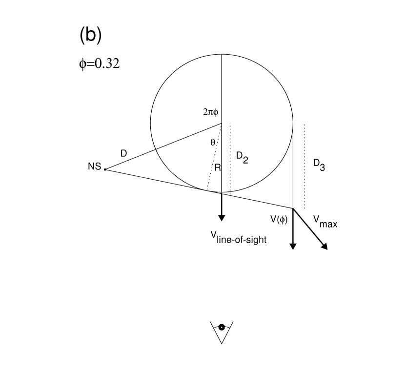
Figure 5:

Figure 6:

Figure 7:

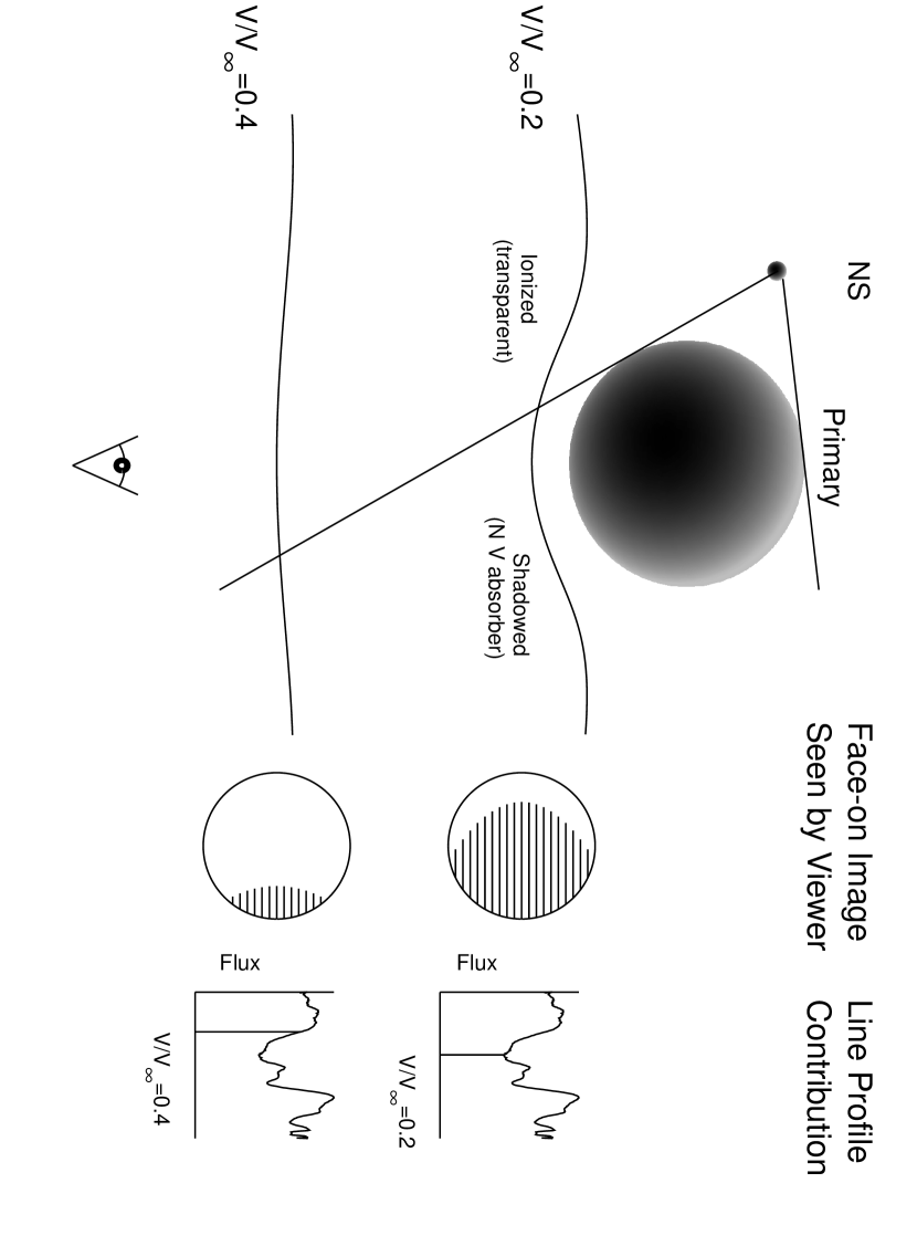
Figure 8:

Figure 9:

Figure 10:

Figure 11:

Figure 12:

References

- (1) Abbott, D.C. 1980, ApJ, 242, 1183
- (2) Abbott, D.C., Telesco, C.M., & Wolff, S.C. 1984, ApJ, 279, 225
- (3) Bieging, J.H., Abbott, D.C., & Churchwell, E.B. 1989, ApJ, 340, 518
- (4) Bjorkman, J.E. 1994, Ap&SS, 221, 443
- (5) Blondin, J.M., Stevens, I.R., & Kallman, T.R. 1991, ApJ, 371, 684
- (6) Blondin, J.M., Kallman, T.R., Fryxell, B.A., & Taam, R.E. 1990, ApJ, 356, 591
- (7) Bomans, D.J., DeBoer, K.S., Koornneef, J., & Grebel, E.K. 1996, A&A 313, 101
- (8) Bondi, H., & Hoyle, F. 1944, MNRAS, 104, 273
- (9) Boroson, B., Kallman, T., Vrtilek, S.D. 1999, in preparation
- (10) Brown, J.C., et al. 1995, A&A, 295, 725
- (11) Buff, J., & McCray, R. 1974, ApJ, 188, L37
- (12) Castor, J. 1970, MNRAS, 149, 11
- (13) Castor, J.I., Abbott, D.C., & Klein, R.I. 1975, ApJ, 195, 157
- (14) Castor, J., & Lamers, H.J.G.L.M., 1979, ApJS, 39, 481
- (15) Corcoran, M.F., et al. 1994, ApJ, 436, L35
- (16) de La Pena, M.D., Nichols-Bohlin, J., Levay, K.L., Michalitsianos, A. 1994, ADASS, 61, 127
- (17) Dupree, A.K. et al. 1980, ApJ, 238, 969
- (18) Fransson, C., & Fabian, A.C. 1980, A&A, 87, 102
- (19) Friend, D.B., & Castor, J. I. 1983, ApJ, 272, 259
- (20) Garmany, C.D., & Conti, P.S. 1985, ApJ, 293, 407
- (21) Groenewegen, M.A.T., & Lamers, H.J.G.L.M. 1989, A&A, 221, 78
- (22) Haberl, F., White, N.E., and Kallman, T.R. 1989, ApJ, 343, 409
- (23) Hammerschlag-Hensberge, G., et al. 1980, A&A, 85, 119
- (24) Harnden, F.R., et al. 1979, ApJ, 234, L51
- (25) Hatchett, S.P. & McCray, R. 1977, ApJ, 211, 552
- (26) Heemskerk, M.H.M. & van Paradijs, J. 1989, A&A, 223, 154
- (27) Howarth, I.D., & Wilson, R. 1983, MNRAS, 204, 1091
- (28) Hutchings, J.B., Crampton, D., & Cowley, A.P. 1978, ApJ, 225, 548
- (29) Kallman, T., & McCray, R. 1982, ApJS, 50, 263
- (30) Kallman, T.R. & White, N.E. 1982, ApJ, 261, L35
- (31) Kaper, L., Hammerschlag-Hensberge, G., & van Loon, J.Th. 1993, A&A 279, 485
- (32) Kelley, R.L., Jernigan, J.G., Levine, A., Petro, D., Rappaport, S.A. 1983, ApJ, 264, 568
- (33) Kudritzki, R.P., Pauldrach, A., & Puls, J. 1987, A&A, 173, 293
- (34) Lamers, H.J.G.L.M., Cerruti-Sola, M., & Perinotto, M. 1987, ApJ, 314, 726
- (35) Lamers, H.J.G.L.M., Snow, T.P., & Lindholm, D.M. 1995, ApJ, 455, 269
- (36) Lang, F.L., Levine, A.M., Butz, M., Hauskins, S., Howe, S., Primini, S.A., Lewin, W.H.G., Baity, W.A., Knight, F.K., Rothschild, R.E., Petterson, J.A. 1981, ApJ, 246, L21
- (37) Levine, A., Rappaport, S., Putney, A., Corbet, R., & Nagase, F. 1991, ApJ, 381, 101
- (38) Li, F., Rappaport, S., & Epstein, A. 1978, Nature, 271, 37
- (39) Lubow, S.H., & Shu, F.H. ApJ, 198, 383
- (40) Lucy, L.B. 1982a, ApJ, 255, 286
- (41) Lucy, L.B., & Solomon, P.M. 1970, ApJ, 159, 879
- (42) Lucy, L.B., & White, R.L. 1980, ApJ, 241, 300
- (43) Massa, D., et al. 1995, ApJ, 452, L53
- (44) MacFarlane, J.J., Cohen, D.H., & Wang, P. 1994, ApJ, 437, 351
- (45) MacGregor, K.B., Hartmann, L, & Raymond, J.C. 1979, ApJ, 231, 514
- (46) McCray, R., Kallman, T.R., Castor, J.I., & Olson, G.L. 1984, ApJ, 282, 245
- (47) Olson, G.L. 1982, ApJ, 255, 267
- (48) Owocki, S.P., Castor, J.I., & Rybicki, G.B. 1988, ApJ 335, 914
- (49) Owocki, S.P., & Rybicki, G.B. 1984, ApJ, 284, 337
- (50) Pauldrach, A.W.A., Kudritzki, R.P., Puls, J., Butler, K., & Hunsinger, J. 1994, A&A, 283, 525
- (51) Pauldrach, A., Puls, J., Kudritzki, R.P., Mendez, R.H., & Heap, S.R. 1988, A&A, 207, 123
- (52) Pauldrach, A. 1987, A&A, 183, 295
- (53) Pauldrach, A., Puls, J., & Kudritzki, R.P. 1986, A&A, 164, 86
- (54) Pietsch, W., Pakull, M., Voges, W., & Staubert, R. 1985, Space Sci. Rev., 40, 371
- (55) Puls, J., Owocki, S.P., & Fullerton, A.W. 1993, A&A, 279, 457
- (56) Seward, F.D., et al. 1979, ApJ, 234, L55
- (57) Press, W.H., Teukolsky, S.A., Vetterling, W.T., & Flannery, B.P. 1992, Numerical Recipes: The Art of Scientific Computing (New York: Cambridge University Press)
- (58) Sunyaev, R., et al. 199a, SvAL, 17 975
- (59) van der Klis, M. et al. 1982, A&A, 106, 339
- (60) Vrtilek, S.D., Boroson, B., McCray, R., Nagase, F., & Cheng, F. 1997, ApJ, 490, 377
- (61) White, N.E., Kallman, T.R., & Swank, J.H. 1983, ApJ, 269, 264
- (62) Wollaert, J.P.M., Lamers, H.J.G.L.M., & de Jager, C. 1988, A&A, 194, 197.
- (63) Woo, J.W., Clark, G.W., & Levine, A.M. 1995, ApJ, 449, 880
- (64) Woo, J.W., Clark, G.W., Levine, A.M., Corbet, R.H., & Nagase, F. 1996, ApJ 467, 811