An analytic approximation of MDM power spectra in four dimensional parameter space

Abstract

An accurate analytic approximation of the transfer function for the power spectra of primordial density perturbations in mixed dark matter models is presented. The fitting formula in a matter-dominated Universe ($\Omega_{0}=\Omega_{M}=1$) is a function of wavenumber $k$, redshift $z$ and four cosmological parameters: the density of massive neutrinos, $\Omega_{\nu}$, the number of massive neutrino species, $N_{\nu}$, the baryon density, $\Omega_{b}$ and the dimensionless Hubble constant, $h$. Our formula is accurate in a broad range of parameters: $k\leq 100\;h/Mpc$, $z\leq 30$, $\Omega_{\nu}\leq 0.5$, $N_{\nu}\leq 3$, $\Omega_{b}\leq 0.3$, $0.3\leq h\leq 0.7$. The deviation of the variance of density fluctuations calculated with our formula from numerical results obtained with CMBfast is less than $6\%$ for the entire range of parameters. It increases with $\Omega_{b}h^{2}$ and is less than $\leq 3\%$ for $\Omega_{b}h^{2}\leq 0.05$.

The performance of the analytic approximation of MDM power spectra proposed here is compared with other approximations found in the literature ([Holtzman 1989, Pogosyan & Starobinsky 1995, Ma 1996, Eisenstein & Hu 1997b]). Our approximation turns out to be closest to numerical results in the parameter space considered here.

1 Introduction

Finding a viable model for the formation of large scale structure (LSS) is an important problem in cosmology. Models with a minimal number of free parameters, such as standard cold dark matter (sCDM) or standard cold plus hot, mixed dark matter (sMDM) only marginally match observational data. Better agreement between predictions and observational data can be achieved in models with a larger numbers of parameters (CDM or MDM with baryons, tilt of primordial power spectrum, 3D curvature, cosmological constant, see, e.g., [Valdarnini et al. 1998] and refs. therein). In view of the growing amount of observational data, we seriously have to discuss the precise quantitative differences between theory and observations for the whole class of available models by varying all the input parameters such as the tilt of primordial spectrum, $n$, the density of cold dark matter, $\Omega_{CDM}$, hot dark matter, $\Omega_{\nu}$, and baryons, $\Omega_{b}$, the vacuum energy or cosmological constant, $\Omega_{\Lambda}$, and the Hubble parameter $h$ ($h=H_{0}/100\;km/s/Mpc$), to find the values which agree best with observations of large scale structure (or even to exclude the whole family of models.).

Publicly available fast codes to calculate the transfer function and power spectrum of fluctuations in the cosmic microwave background (CMB) ([Seljak & Zaldarriaga 1996], CMBfast) are an essential ingredient in this process. But even CMBfast is too bulky and too slow for an effective search of cosmological parameters by means of a $\chi^{2}$-minimization, like that of Marquardt (see [Press et al. 1992]). To solve this problem, analytic approximations of the transfer function are of great value. Recently, such an approximation has been proposed by [Eisenstein & Hu 1997b] (this reference is denoted by EH2 in the sequel). Previously, approximations by [Holtzman 1989, Pogosyan & Starobinsky 1995, Ma 1996] have been used.

Holtzman’s approximation is very accurate but it is an approximation for fixed cosmological parameters. Therefore it can not be useful for the purpose mentioned above. The analytic approximation by [Pogosyan & Starobinsky 1995] is valid in the 2-dimensional parameter space $(\Omega_{\nu},h)$, and $z$ (the redshift). It has the correct asymptotic behavior at small and large $k$, but the systematic error of the transfer function $T(k)$ is relatively large (10%-15%) in the important range of scales $0.3\leq k\leq 10\;h/$Mpc. This error, however introduces discrepancies of 4% to 10% in $\sigma_{R}$ which represents an integral over $k$. Ma’s analytic approximation is slightly more accurate in this range, but has an incorrect asymptotic behavior at large $k$, hence it cannot be used for the analysis of the formation of small scale objects (QSO, damped $Ly_{\alpha}$ systems, $Ly_{\alpha}$ clouds etc.).

Another weak point of these analytic approximations is their lack of dependence on the baryon density. Sugiyama’s correction of the CDM transfer function in the presence of baryons ([Bardeen et al. 1986, Sugiyama 1995]) works well only for low baryonic content. Recent data on the high-redshift deuterium abundance ([Tytler et al. 1996]), on clustering at $100$Mpc$/h$ ([Eisenstein et al. 1997]) and new theoretical interpretations of the $Ly_{\alpha}$ forest ([Weinberg et al. 1997]) suggest that $\Omega_{b}$ may be higher than the standard nucleosynthesis value. Therefore pure CDM and MDM models have to be modified. (Instead of raising $\Omega_{b}$, one can also look for other solutions, like, e.g. a cosmological constant, see below.)

For CDM this has been achieved by Eisenstein $\&$ Hu (1996, 1997a) using an analytical approach for the description of small scale cosmological perturbations in the photon-baryon-CDM system. Their analytic approximation for the matter transfer function in 2-dimensional parameter space ($\Omega_{M}h^{2}$, $\Omega_{b}/\Omega_{M}$) reproduces acoustic oscillations, and is quite accurate for $z<30$ (the residuals are smaller than 5%) in the range $0.025\leq\Omega_{M}h^{2}\leq 0.25$, $0\leq\Omega_{b}/\Omega_{M}\leq 0.5$, where $\Omega_{M}$ is the matter density parameter.

In EH2 an analytic approximation of the matter transfer function for MDM models is proposed for a wide range of parameters ($0.06\leq\Omega_{M}h^{2}\leq 0.4$, $\Omega_{b}/\Omega_{M}\leq 0.3$, $\Omega_{\nu}/\Omega_{M}\leq 0.3$ and $z\leq 30$). It is more accurate than previous approximations by [Pogosyan & Starobinsky 1995, Ma 1996] but not as precise as the one for the CDM+baryon model. The baryon oscillations are mimicked by a smooth function, therefore the approximation looses accuracy in the important range $0.03\leq k\leq 0.5~{}h/$Mpc. For the parameter choice $\Omega_{M}=1$, $\Omega_{\nu}=0.2$, $\Omega_{b}=0.12$, $h=0.5$, e.g., the systematic residuals are about 6% on these scales. For higher $\Omega_{\nu}$ and $\Omega_{b}$ they become even larger.

For models with cosmological constant, the motivation to go to high values for $\Omega_{\nu}$ and $\Omega_{b}$ is lost, and the parameter space investigated in EH2 is sufficient. Models without cosmological constant, however, tend to require relatively high baryon or HDM content. In this paper, our goal is thus to construct a very precise analytic approximation for the redshift dependent transfer function in the 4-dimensional space of spatially flat matter dominated MDM models, $T_{MDM}(k;\Omega_{\nu},N_{\nu},\Omega_{b},h;z)$, which is valid for $\Omega_{M}=1$ and allows for high values of $\Omega_{\nu}$ and $\Omega_{b}$. In order to keep the baryonic features, we will use the EH1 transfer function for the cold particles+baryon system, $T_{CDM+b}(k;\Omega_{b},h)$, and then correct it for the presence of HDM by a function $D(k;\Omega_{\nu},N_{\nu},\Omega_{b},h;z)$, making use of the exact asymptotic solutions. The resulting MDM transfer function is the product $T_{MDM}(k)=T_{CDM+b}(k)D(k)$.

To compare our approximation with the numerical result, we use the publicly available code ’CMBfast’ by Seljak $\&$ Zaldarriaga 1996.

The paper is organized as follows: In Section 2 a short description of the physical parameters which affect the shape of the MDM transfer function is given. In Section 3 we derive the analytic approximation for the function $D(k)$. The precision of our approximation for $T_{MDM}(k)$, the parameter range where it is applicable, and a comparison with the other results are discussed in Sections 4 and 5. In Section 6 we present our conclusions.

2 Physical scales which determine the form of MDM transfer function

We assume the usual cosmological paradigm: scalar primordial density perturbations which are generated in the early Universe, evolve in a multicomponent medium of relativistic (photons and massless neutrinos) and non-relativistic (baryons, massive neutrinos and CDM) particles. Non-relativistic matter dominates the density today, $\Omega_{M}=\Omega_{b}+\Omega_{\nu}+\Omega_{CDM}$. This model is usually called ’mixed dark matter’ (MDM). The total energy density may also include a vacuum energy, so that $\Omega_{0}=\Omega_{M}+\Omega_{\Lambda}$. However, for reasons mentioned in the introduction, here we investigate the case of a matter-dominated flat Universe with $\Omega_{M}=1$ and $\Omega_{\Lambda}=0$. Even though $\Omega_{\Lambda}\neq 0$ seems to be favored by some of the present data, our main point, allowing for high values of $\Omega_{b}$, is not important in this case and the approximations by EH2 can be used.

Models with hot dark matter or MDM have been described in the literature by [Fang, Xiang & Li 1984, Shafi & Stecker 1984, Valdarnini & Bonometto 1985, Holtzman 1989, Lukash 1991], Davis, Summers $\&$ Schlegel 1992, [Schaefer & Shafi 1992, Van Dalen & Schaefer 1992], Pogosyan $\&$ Starobinsky 1993, 1995, [Novosyadlyj 1994], Ma $\&$ Bertschinger 1994, 1995, [Seljak & Zaldarriaga 1996], EH2, [Valdarnini et al. 1998] and refs. therein. Below, we simply present the physical parameters which determine the shape of the MDM transfer function and which will be used explicitly in the approximation which we derive here.

Figure 1: The transfer function of density perturbations of CDM, baryons and HDM at $z=10$ (calculated numerically).

Figure 2: The same as in Fig.1 but for z=0.

Since cosmological perturbations cannot grow significantly in a radiation dominated universe, an important parameter is the time of equality between the densities of matter and radiation

$$z_{eq}=\frac{2.4\times 10^{4}}{1-N_{\nu}/7.4}h^{2}t_{\gamma}^{-4}-1,$$

where $t_{\gamma}\equiv T_{\gamma}/2.726K$ is the CMB temperature today, $N_{\nu}$=1, 2 or 3 is the number of species of massive neutrinos with equal mass (the number of massless neutrino species is then $3-N_{\nu}$). The scale of the particle horizon at this epoch,

$$k_{eq}=4.7\times 10^{-4}\sqrt{1+z_{eq}}\;h/Mpc,$$

is imprinted in the matter transfer function: perturbations on smaller scales ($k>k_{eq}$) can only start growing after $z_{eq}$, while those on larger scales ($k<k_{eq}$) keep growing at any time. This leads to the suppression of the transfer function at $k>k_{eq}$. After $z_{eq}$ the fluctuations in the CDM component are gravitationally unstable on all scales. The scale $k_{eq}$ is thus the single physical parameter which determines the form of the CDM transfer function.

The transfer function for HDM ($\nu$) is more complicated because two more physical scales enter the problem. The time and horizon scale when neutrino become non-relativistic ($m_{\nu}\simeq 3T_{\nu}$) are given by

$$z_{nr}=x_{\nu}(1+z_{eq})-1\;\;,$$

$$k_{nr}=3.3\times 10^{-4}\sqrt{x_{\nu}(1+x_{\nu})(1+z_{eq}})\;h/Mpc,$$

where $x_{\nu}\equiv\Omega_{\nu}/\Omega_{\nu\;eq}\;$, $\;\;\Omega_{\nu\;eq}\simeq N_{\nu}/(7.4-N_{\nu})$ is the density parameter for a neutrino component becoming non-relativistic just at $z_{eq}$. The neutrino mass can be expressed in terms of $\Omega_{\nu}$ and $N_{\nu}$ as ([Peebles 1993]) $m_{\nu}=94\Omega_{\nu}h^{2}N_{\nu}^{-1}t_{\gamma}^{-3}\;$eV.

The neutrino free-streaming (or Jeans) scale at $z\leq z_{nr}$ is

$$k_{F}(z)\simeq 59\sqrt{{1\over 1+z_{eq}}+{1\over 1+z}}\;\Omega_{\nu}N_{\nu}^{-1}t_{\gamma}^{-4}\;h^{3}/Mpc,$$

which corresponds to the distance a neutrino travels in one Hubble time, with the characteristic velocity $v_{\nu}\simeq{1\over x_{\nu}}{1+z\over 1+z_{eq}}.$ Obviously, $k_{F}\geq k_{nr}$, and $k_{nr}{}^{>}_{<}k_{eq}$ for $\Omega_{\nu}{}^{>}_{<}\Omega_{\nu\;eq}\;$.

The amplitude of $\nu$-density perturbation on small scales ($k>k_{nr}$) is reduced in comparison with large scales ($k<k_{nr}$). For scales larger than the free-streaming scale ($k<k_{F}$) the amplitude of density perturbations grows in all components like $(1+z)^{-1}$ after $z_{eq}$. Perturbations on scales below the free-streaming scale ($k>k_{F}$) are suppressed by free streaming which is imprinted in the transfer function of HDM. Thus the latter should be parameterized by two ratios: $k/k_{nr}$ and $k/k_{F}$.

The transfer function of the baryon component is determined by the sound horizon and the Silk damping scale at the time of recombination (for details see EH1).

In reality the transfer function of each component is more complicated due to interactions between them. At late time ($z<20$), the baryonic transfer function is practically equal to the one of CDM, for models with $\Omega_{b}<\Omega_{CDM}$ (see Figs. 1,2). After $z_{eq}$, the free-streaming scale decreases with time (neutrino momenta decay with the expansion of the Universe whereas the Hubble time grows only as the square root of the scale factor, see Eq. (4)), and neutrino density perturbations at smaller and smaller scales become gravitationally unstable and cluster with the CDM+baryon component. Today the $\nu$ free-streaming scale may lie in the range of galaxy to clusters scales depending on the $\nu$ mass. On smaller scales the growing mode of perturbation is concentrated in the CDM and baryon components. Matter density perturbation on these scales grow like $\sim t^{\alpha}$, where $\alpha=(\sqrt{25-24\Omega_{\nu}}-1)/6$ ([Doroshkevich et al. 1980]).

3 An analytic approximation for the MDM transfer function

To construct the MDM transfer function we use the analytic approximation of EH1 for the transfer function of cold particles plus baryons and correct it for the presence of a $\nu$-component like [Pogosyan & Starobinsky 1995] and [Ma 1996]:

$$T_{MDM}(k)=T_{CDM+b}(k)D(k)~{}.$$

The function $D(k)$ must have the following asymptotics:

$$D(k\ll k_{nr})=1,$$

$$D(k\gg k_{F})=(1-\Omega_{\nu})\left({1+z\over 1+z_{eq}}\right)^{\beta},$$

where $\beta=1-1.5\alpha$. After some numerical experimentation we arrive at the following ansatz which satisfies these asymptotics

$$D(k)=\left[{1+(1-\Omega_{\nu})^{1/\beta}{1+z\over 1+z_{eq}}({k_{F}\over k_{nr}})^{3}\Sigma_{i=1}^{3}\alpha_{i}\left({k\over k_{F}}\right)^{i}\over 1+(\alpha_{4}k/k_{nr})^{3}}\right]^{\beta}.$$

We minimize the residuals in intermediate region ($k_{nr}<k<k_{F}$) by determining $\alpha_{i}$ as best fit coefficients by comparison with the numerical results.

By $\chi^{2}$ minimization ([Press et al. 1992]) we first determine the dependence of the coefficients $\alpha_{i}$ on $\Omega_{\nu}$ keeping all other parameters fixed, to obtain an analytic approximation $\alpha_{i}(\Omega_{\nu},z)$. The main dependence of $T_{MDM}(k)$ on $\Omega_{b},\;N_{\nu},\;h$ and $z$ is taken care of by the dependence of $T_{CDM+b}$, $k_{nr}$, $k_{F}$ and of the asymptotic solution on these parameters. We then correct $\alpha_{i}$ by minimization of the residuals to include the slight dependence on these parameters.

Finally, the correction coefficients have the following form:

$$\alpha_{i}=a_{i}A_{i}(z)B_{i}(\Omega_{b})C_{i}(h)D_{i}(N_{\nu}),$$

where $a_{i}=a_{i}(\Omega_{\nu})$, $A_{i}(0)=B_{i}(0.06)=C_{i}(0.5)=D_{i}(1)=1$. The functions $A_{i}$ depend also on $\Omega_{\nu}$.

For all our calculations we assume a CMB temperature of $T_{\gamma}=2.726K$ ([Mather et al. 1994, Kogut et al. 1996]).

3.1 Dependence on $\Omega_{\nu}$ and $z$.

We first set $h=0.5$, $\Omega_{b}=0.06$, $N_{\nu}=1$ and determine $\alpha_{i}$ for $\Omega_{\nu}=0.1,\;0.2,\;0.3,\;0.4,\;0.5$ and $z=0,\;10,\;20$. We then approximate $D(k)$ by setting $\alpha_{i}=a_{i}A_{i}(z)$, where $A_{i}(z)=(1+z)^{b_{i}+c_{i}(1+z)}$. The dependences of $a_{i}$, $b_{i}$ and $c_{i}$ on $\Omega_{\nu}$, as well as $B_{i}(\Omega_{b})$, $C_{i}(h)$ and $D_{i}(N_{\nu})$ are given in the Appendix. The functions $D(k)$ for different $\Omega_{\nu}$ and its fractional residuals are shown in Figs. 3 and 4.

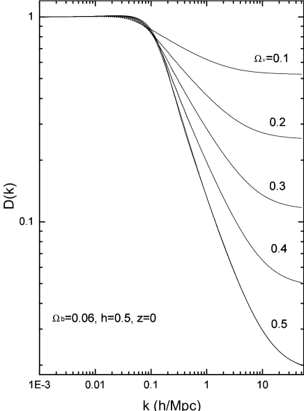
Figure 3: $D(k)=T_{MDM}(k)/T_{CDM+b}(k)$ as calculated numerically (solid line) and our analytic approximation (dotted line) for different values of $\Omega_{\nu}$. The numerical results and the approximations overlay perfectly.

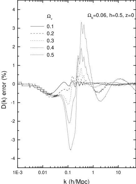
Figure 4: Fractional residuals of $D(k)$ given by $(D(k)-D_{CMBfast}(k))/D_{CMBfast}(k)$ for different values of $\Omega_{\nu}$.

We now analyze the accuracy of our analytic approximation for the MDM transfer function $T_{MDM}(k)=T_{CDM+b}D(k)$ which in addition to the errors in $D(k)$ contains also those of $T_{CDM+b}(k)$ (EH1). We define the fractional residuals for $T_{MDM}(k)$ by $(T(k)-T_{CMBfast}(k))/T_{CMBfast}(k)$. In Fig. 5 the numerical result for $T_{MDM}(k)$ (thick solid lines) and the analytic approximations (dotted thin lines) are shown for different $\Omega_{\nu}$. The fractional residuals for the latter are given in Fig. 6. Our analytic approximation of $T_{MDM}(k)$ is sufficiently accurate for a wide range of redshifts (see Fig.7). For $z\leq 30$ the fractional residuals do not change by more than 2% and stay small.

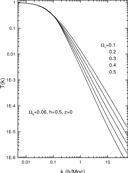
Figure 5: The numerical MDM transfer function at $z=0$ (thick solid lines) and the analytic approximations $T_{MDM}(k)=T_{CDM+b}D(k)$ (dotted thin lines, which perfectly overlay with the numerical result).

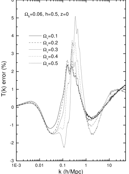
Figure 6: The fractional residuals of $T(k)$ given by $(T(k)-T_{CMBfast}(k))/T_{CMBfast}(k)$ for different values of $\Omega_{\nu}$.

.

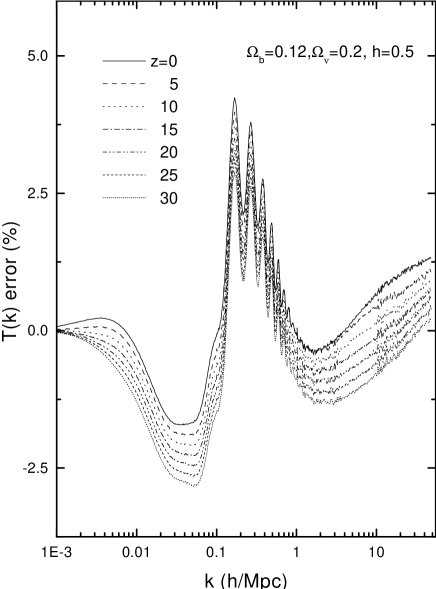
Figure 7: Fractional residuals of the analytic approximation for the MDM transfer function at different redshifts.

3.2 Dependence on $\Omega_{b}$ and $h$.

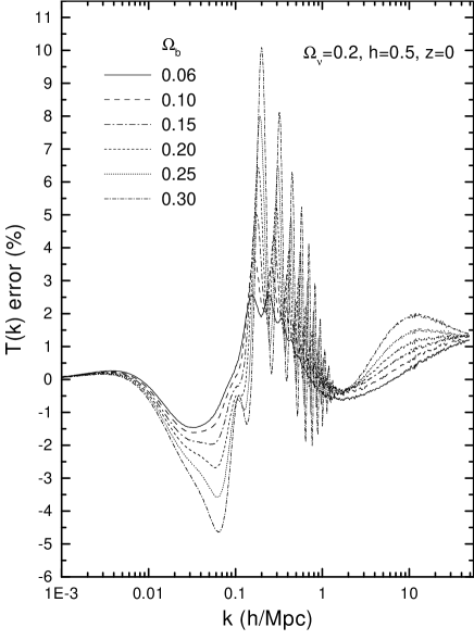
Figure 8: Fractional residuals of the analytic approximation of the MDM transfer function for different values of $\Omega_{b}$.

We now vary $\Omega_{b}$ fixing different values of $\Omega_{\nu}$ and setting the other parameters $h=0.5$, $N_{\nu}=1$. We analyze the ratio $D(k;\Omega_{\nu},\Omega_{b})/D(k;\Omega_{\nu},\Omega_{b}=0.06)$. Since the dominant dependence of $T_{MDM}(k)$ on $\Omega_{b}$ is already taken care of in $T_{CDM+b}(k)$, $D(k)$ is only slightly corrected for this parameter. Correction factors $B_{i}(\Omega_{b})$ ($\sim 1$) as a second order polynomial dependence on $\Omega_{b}/0.06$ with best-fit coefficients are presented in the Appendix. The fractional residuals of $T_{MDM}(k)$ for different $\Omega_{b}$ are shown in Fig. 8.

The maximum of the residuals grows for higher baryon fractions. This is due to the acoustic oscillations which become more prominent and their analytic modeling in MDM models is more complicated.

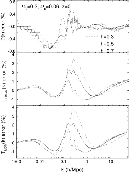
Figure 9: Fractional residuals of the analytic approximation of $D(k)$, $T_{CDM+b}(k)$ and $T_{MDM}(k)$ transfer function for different values of the Hubble parameter, $h$.

A similar situation occurs also for the dependence of $T_{MDM}(k)$ on $h$. Since the $h$-dependence is included properly in $k_{F}$ and $k_{nr}$, $D(k)$ does not require any correction in the asymptotic regimes. Only a tiny correction of $D(k)$ in the intermediate range, $k$ ($0.01<k<1$) is necessary to minimize the residuals. By numerical experiments we find that this can be achieved by multiplying $\alpha_{1},...\alpha_{4}$ by the factors $C_{i}(h)$ which are approximated by second order polynomial on $h/0.5$ with coefficients determined by $\chi^{2}$ minimization (see Appendix). The fractional residuals of $D(k)$ for different $h$ are shown in Fig. 9 (top panel), they remain stable in the range $0.3\leq h\leq 0.7$. But the fractional residuals of $T_{MDM}(k)$ slightly grow (about 2-3%, bottom Fig. 9) in the range $0.1\leq k\leq 1$ when $h$ grows from 0.3 to 0.7. This is caused by the fractional residuals of $T_{CDM+b}(k)$ (see middle panel).

3.3 Dependence on $N_{\nu}$.

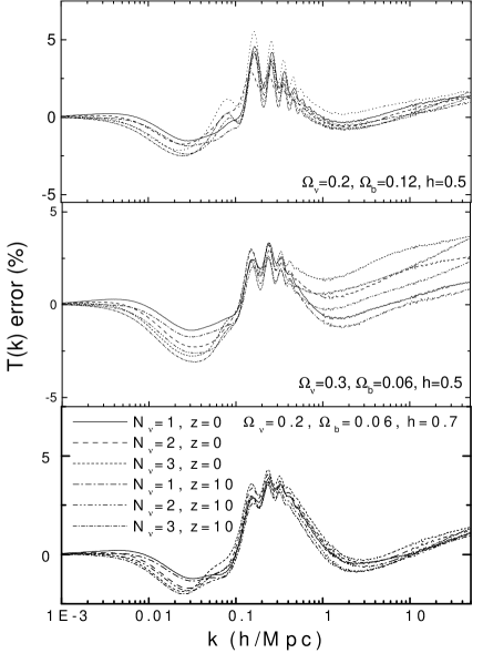
Figure 10: Fractional residuals for the analytic approximation of the MDM transfer function of density perturbations for different numbers of massive neutrino species, $N_{\nu}$, in models with different values of $\Omega_{\nu}$, $\Omega_{b}$ and $h$.

The dependence of $D(k)$ on the number of massive neutrino species, $N_{\nu}$, is taken into account in our analytic approximation by the corresponding dependence of the physical parameters $k_{nr}$ and $k_{F}$ (see Eq.(6)). It has the correct asymptotic behaviour on small and large scales but rather large residuals in the intermediate region $0.01<k<10$. Therefore, the coefficients $\alpha_{i}$ ($i=1,...,4$) must be corrected for $N_{\nu}$. To achieve this, we multiply each $\alpha_{i}$ by a factor $D_{i}(N_{\nu})$ ($\sim 1$) which we determine by $\chi^{2}$ minimization. These factors depend on $N_{\nu}$ as second order polynomials. They are given in the Appendix. In Fig. 10 we show the fractional residuals of $T_{MDM}(k)$ for different numbers of massive neutrino species, $N_{\nu}$, and several values of the parameters $\Omega_{\nu}$, $\Omega_{b}$, $h$ and $z$. The performance for $N_{\nu}=2,3$ is approximately the same as for $N_{\nu}=1$.

4 Performance

Figure 11: The variance of density perturbations smoothed by a top-hat filter of radius $R$ for different MDM models. Numerical transfer functions $T_{MDM}$ are shown as thick lines and the analytic approximations $T_{MDM}(k)=T_{CDM+b}D(k)$ are thin lines which are superimposed on the numerical results (The residuals are not visible on this scale.).

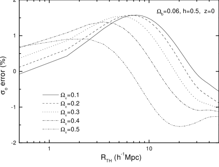
Figure 12: The fractional residuals of $\sigma(R)$ defined by $(\sigma(R)-\sigma_{CMBfast}(R))/\sigma_{CMBfast}(R)$ for different values of $\Omega_{\nu}$ with all other parameters fixed.

The analytic approximation of $D(k)$ proposed here has maximal fractional residuals of less than $5\%$ in the range $0.01\leq k\leq 1$. It is oscillating around the exact numerical result (see Fig. 4), which essentially reduces the fractional residuals of integral quantities like $\sigma(R)$. Indeed, the mean square density perturbation smoothed by a top-hat filter of radius $R$

$$\sigma^{2}(R)={1\over 2\pi^{2}}\int_{0}^{\infty}k^{2}P(k)W^{2}(kR)dk,$$

where $W(x)=3(\sin x-x\cos x)/x^{3}$, $P(k)=AkT_{MDM}^{2}(k)$ (Fig.11) has fractional residuals which are only about half the residuals of the transfer function (Fig.12). To normalize the power spectrum to the 4-year COBE data we have used the fitting formula by [Bunn and White 1997].

The accuracy of $\sigma(R)$ obtained by our analytic approximation is better than $2\%$ for a wide range of $\Omega_{\nu}$ for $\Omega_{b}=0.06$ and $h=0.5$. Increasing $\Omega_{b}$ slightly degrades the approximation for $N_{\nu}>1$, but even for a baryon content as high as $\Omega_{b}\sim 0.2$, the fractional residuals of $\sigma(R)$ do not exceed $5\%$. Changing $h$ in the range $0.3-0.7$ and $N_{\nu}=1-3$ do also not reduce the accuracy of $\sigma(R)$ beyond this limit.

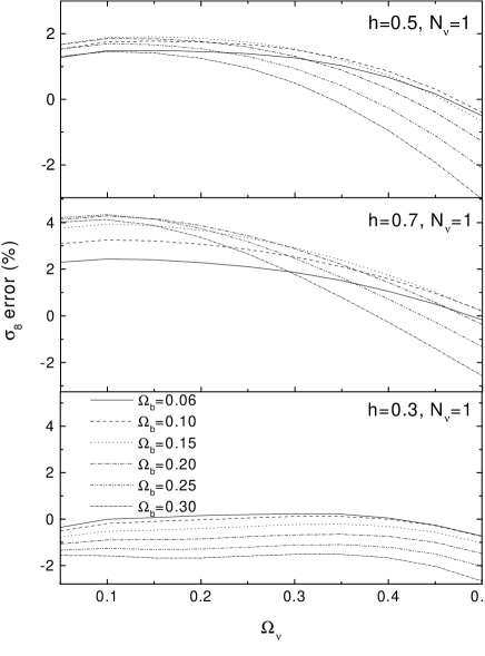
Figure 13: Deviation of $\sigma_{8}$ of our analytic approximation for $T_{MDM}(k)$ from the numerical result for different values of $\Omega_{\nu}$, $\Omega_{b}$ and $h$ ($N_{\nu}=1$).

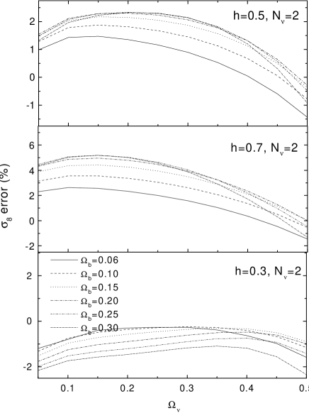
Figure 14: Same as Fig.13, but for $N_{\nu}=2$.

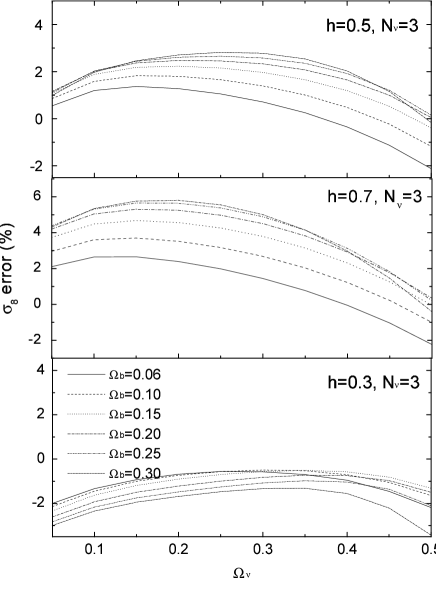
Figure 15: Same as Fig.13, but for $N_{\nu}=3$.

We now evaluate the quality and fitness of our approximation in the four dimensional space of parameters. We see in Fig.12 that the largest errors of our approximation for $\sigma(R)$ come from scales of $\sim 5-10h^{-1}Mpc$. Since these scales are used for the evaluation of the density perturbation amplitude on galaxy cluster scale, it is important to know how accurately we reproduce them. The quantity $\sigma_{8}\equiv\sigma(8h^{-1}Mpc)$ is actually the most often used value to test models. We calculate it for the set of parameters $0.05\leq\Omega_{\nu}\leq 0.5$, $0.06\leq\Omega_{b}\leq 0.3$, $0.3\leq h\leq 0.7$ and $N_{\nu}=1,\;2,\;3$ by means of our analytic approximation and numerically. The relative deviations of $\sigma_{8}$ calculated with our $T_{MDM}(k)$ from the numerical results are shown in Fig.13-15.

As one can see from Fig. 13, for $0.3\leq h\leq 0.7$ and $\Omega_{b}h^{2}\leq 0.15$ the largest error in $\sigma_{8}$ for models with one sort of massive neutrinos $N_{\nu}=1$ does not exceed $4.5\%$ for $\Omega_{\nu}\leq 0.5$. Thus, for values of $h$ which are followed by direct measurements of the Hubble constant, the range of $\Omega_{b}h^{2}$ where the analytic approximation is very accurate for $\Omega_{\nu}\leq 0.5$ is six times as wide as the range given by nucleosynthesis constraints, ($\Omega_{b}h^{2}\leq 0.024$, [Tytler et al. 1996]). This is important if one wants to determine cosmological parameters by the minimization of the difference between the observed and predicted characteristics of the large scale structure of the Universe.

For models with more than one species of massive neutrinos of equal mass ($N_{\nu}=2,3$), the accuracy of our analytic approximation is slightly worse (Fig. 14, 15). But even for extremely high values of parameters $\Omega_{b}=0.3$, $h=0.7$, $N_{\nu}=3$ the error in $\sigma_{8}$ does not exceed $6\%$.

In redshift space the accuracy of our analytic approximation is stable and quite high for redshifts of up to $z=30$.

5 Comparison with other analytic approximations

Figure 16: Fractional residuals of $\sigma(R)$ calculated by the analytic approximation of EH2 for the same parameters as in Fig. 12.

Figure 17: Fractional residuals of the analytic approximation by EH2 of the MDM transfer function for the same parameters as in Fig.16. For comparison see Fig.6.

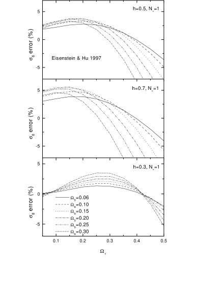
Figure 18: Deviation of $\sigma_{8}$ as obtained by the fitting formula of EH2 from numerical results for different values of $\Omega_{\nu}$, $\Omega_{b}$ and $h$ ($N_{\nu}=1$). See Fig. 13 for comparison.

We now compare the accuracy of our analytic approximation with those cited in the introduction. For comparison with Fig. 12 the fractional residuals of $\sigma(R)$ calculated with the analytic approximation of $T_{MDM}(k)$ by EH2 are presented in Fig. 16. Their approximation is only slightly less accurate ($\sim 3\%$) at scales $\geq 10Mpc/h$. In Fig. 17 the fractional residuals of the EH2 approximation of $T_{MDM}(k)$ are shown for the same cosmological parameters as in Fig. 16. For $\Omega_{\nu}=0.5$ (which is not shown) the deviation from the numerical result is $\geq 50\%$ at $k\geq 1h^{-1}$Mpc, and the EH2 approximation completely breaks down in this region of parameter space.

The analog to Fig. 13 ($\sigma_{8}$) for the fitting formula of EH2 is shown in Fig. 18 for different values of $\Omega_{b}$, $\Omega_{\nu}$ and $h$. Our analytic approximation of $T_{MDM}(k)$ is more accurate than EH2 in the range $0.3\leq\Omega_{\nu}\leq 0.5$ for all $\Omega_{b}$ ($\leq 0.3$). For $\Omega_{\nu}\leq 0.3$ the accuracies of $\sigma_{8}$ are comparable.

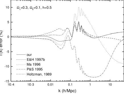
Figure 19: Fractional residuals of different analytic approximations for the MDM transfer function at $z=0$ for one flavor of massive neutrinos.

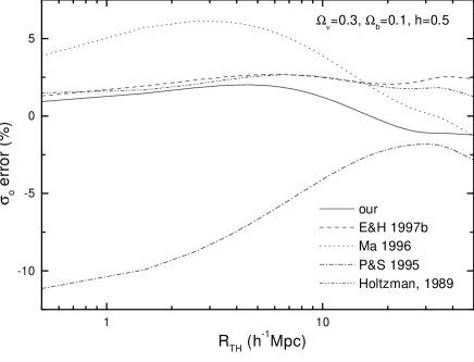
Figure 20: Fractional residuals of $\sigma(R)$ calculated with the same analytic approximations as Fig. 19.

To compare the accuracy of the analytic approximations for $T_{MDM}(k)$ given by [Holtzman 1989], Pogosyan $\&$ Starobinsky 1995, [Ma 1996], EH2 with the one presented here, we determine the transfer functions for the fixed set of parameters ($\Omega_{\nu}=0.3$, $\Omega_{b}=0.1$, $N_{\nu}=1$, $h=0.5$) for which all of them are reasonably accurate. Their deviations (in %) from the numerical transfer function are shown in Fig. 19. The deviation of the variance of density fluctuations for different smoothing scales from the numerical result is shown in Fig. 20. Clearly, our analytic approximation of $T_{MDM}(k)$ opens the possibility to determine the spectrum and its momenta more accurate in wider range of scales and parameters.

6 Conclusions

We propose an analytic approximation for the linear power spectrum of density perturbations in MDM models based on a correction of the approximation by EH1 for CDM plus baryons. Our formula is more accurate than previous ones ([Pogosyan & Starobinsky 1995, Ma 1996], EH2) for matter dominated Universes ($\Omega_{M}=1$) in a wide range of parameters: $0\leq\Omega_{\nu}\leq 0.5$, $0\leq\Omega_{b}\leq 0.3$, $0.3\leq h\leq 0.7$ and $N_{\nu}\leq 3$. For models with one, two or three flavors of massive neutrinos ($N_{\nu}=1,\;2,\;3$) it is significantly more accurate than the approximation by EH2 and has a relative error $\leq 6\%$ in a wider range for $\Omega_{\nu}$ (see Figs. 13, 18).

The analytic formula given in this paper provides an essential tool for testing a broad class of MDM models by comparison with different observations like the galaxy power spectrum, cluster abundances and evolution, clustering properties of Ly-$\alpha$ lines etc. Results of such an analysis are presented elsewhere.

Our analytic approximation for $T_{MDM}(k)$ is available in the form of a FORTRAN code and can be requested at novos@astro.franko.lviv.ua or copied from http://mykonos.unige.ch/$\boldmath{\sim}$durrer/

Acknowledgments This work is part of a project supported by the Swiss National Science Foundation (grant NSF 7IP050163). B.N. is also grateful to DAAD for financial support (Ref. 325) and AIP for hospitality, where the bulk of the numerical calculations were performed. V.L. acknowledges a partial support of the Russian Foundation for Basic Research (96-02-16689a).

Appendix

The best fit coefficients $a_{i}(\Omega_{\nu})$, $b_{i}(\Omega_{\nu})$, $c_{i}(\Omega_{\nu})$, $B_{i}(\Omega_{b})$, $C_{i}(h)$ and $D_{i}(N_{\nu})$:

$$a_{1}=1.24198-3.88787\Omega_{\nu}+28.33592\Omega_{\nu}^{2}-70.9063\Omega_{\nu}^{2}+84.15833\Omega_{\nu}^{4}-41.16667\Omega_{\nu}^{5}\;,$$

$$a_{2}=0.7295-3.6176\Omega_{\nu}+21.45834\Omega_{\nu}^{2}-54.63036\Omega_{\nu}^{3}+70.80274\Omega_{\nu}^{4}-35.20905\Omega_{\nu}^{5}\;,$$

$$a_{3}=0.28283-0.53987\Omega_{\nu}+5.80084\Omega_{\nu}^{2}-14.18221\Omega_{\nu}^{3}+16.85506\Omega_{\nu}^{4}-8.77643\Omega_{\nu}^{5}\;,$$

$$a_{4}=0.48431+1.89092\Omega_{\nu}-4.04224\Omega_{\nu}^{2}+8.09669\Omega_{\nu}^{3}-10.05315\Omega_{\nu}^{4}+5.34405\Omega_{\nu}^{5}~{}.$$

$$b_{1}=0.2667-1.67\Omega_{\nu}+3.56\Omega_{\nu}^{2}-3.1\Omega_{\nu}^{3}\;,$$

$$c_{1}=0.008-0.055\Omega_{\nu}+0.135\Omega_{\nu}^{2}-0.124\Omega_{\nu}^{3}\;,$$

$$b_{2}=0.226-0.47\Omega_{\nu}+1.27\Omega_{\nu}^{2}-1.39\Omega_{\nu}^{3}\;,$$

$$c_{2}=0.004-0.026\Omega_{\nu}+0.053\Omega_{\nu}^{2}-0.039\Omega_{\nu}^{3}\;,$$

$$b_{3}=0.076-0.258\Omega_{\nu}+0.215\Omega_{\nu}2\;,$$

$$c_{3}=0.0026-0.0205\Omega_{\nu}+0.055\Omega_{\nu}^{2}-0.051\Omega_{\nu}^{3}\;,$$

$$b_{4}=0.0158-0.055\Omega_{\nu}+0.0228\Omega_{\nu}^{2}\;,$$

$$c_{4}=0.00094-0.0072\Omega_{\nu}+0.018\Omega_{\nu}^{2}-0.016\Omega_{\nu}^{3}~{}.$$

$$B_{1}(\Omega_{b})=1.202-0.2065(\Omega_{b}/0.06)+0.005(\Omega_{b}/0.06)^{2}\;,$$

$$B_{2}(\Omega_{b})=1.033-0.036(\Omega_{b}/0.06)+0.003(\Omega_{b}/0.06)^{2}\;,$$

$$B_{3}(\Omega_{b})=1.166-0.17(\Omega_{b}/0.06)+0.005(\Omega_{b}/0.06)^{2}\;,$$

$$B_{4}(\Omega_{b})=0.97985+0.01525(\Omega_{b}/0.06)+0.00626(\Omega_{b}/0.06)^{2}~{}.$$

$$C_{1}(h)=1.09-0.09(h/0.5)\;,$$

$$C_{2}(h)=1.65-0.88(h/0.5)+0.23(h/0.5)^{2}\;,$$

$$C_{3}(h)=1.055-0.055(h/0.5)\;,$$

$$C_{4}(h)=0.981+0.03(h/0.5)-0.012(h/0.5)^{2}~{}.$$

$$D_{1}(N_{\nu})=1.315-0.431N_{\nu}+0.116N_{\nu}^{2}\;,$$

$$D_{2}(N_{\nu})=1.108-0.225N_{\nu}+0.117N_{\nu}^{2}\;,$$

$$D_{3}(N_{\nu})=1.316-0.432N_{\nu}+0.116N_{\nu}^{2}\;,$$

$$D_{4}(N_{\nu})=1.256-0.302N_{\nu}+0.046N_{\nu}^{2}~{}.$$

References

- [Bardeen et al. 1986] Bardeen, J.M., Bond, J.R., Kaiser, N., and Szalay, A.S. 1986, ApJ, 304, 15
- [Bond & Szalay 1983] Bond, J.R., & Szalay, A.S. 1983, ApJ, 274, 443
- [Bunn and White 1997] Bunn, E.F., & White, M. 1997, ApJ, 480, 6
- [Davis, Summers & Schlegel 1992] Davis, M., Summers, F.J., & Schlegel, D. 1992, Nature, 359, 393
- [Doroshkevich et al. 1980] Doroshkevich, A.G., Zeldovich, Ya.B., Sunyaev, R.A. & Khlopov M.Yu. 1980, Sov.Astron. Lett., 6, 252
- [Eisenstein & Hu 1996] Eisenstein, D.J. & Hu, W. 1996, ApJ, 471, 542
- [Eisenstein & Hu 1997a] Eisenstein, D.J. & Hu, W. 1997a, astro-ph/9709112 (EH1)
- [Eisenstein & Hu 1997b] Eisenstein, D.J. & Hu, W. 1997b, astro-ph/9710252 (EH2)
- [Eisenstein et al. 1997] Eisenstein, D.J., Hu, W., Silk, J., Szalay, A.S. 1997, astro-ph/9710303
- [Fang, Xiang & Li 1984] Fang, L.Z., Xiang, S.P., & Li, S.X. 1984, AA140, 77
- [Holtzman 1989] Holtzman, J.A. 1989, ApJSS, 71, 1
- [Kogut et al. 1996] Kogut, A., et al. 1996, ApJ, 470, 653
- [Lukash 1991] Lukash, V.N. 1991, Annals New York Acad. of Sci., 647, 659
- [Ma 1996] Ma, C.-P. 1996, ApJ, 471, 13 (astro-ph/9605198)
- [Ma & Bertschinger 1994] Ma, C.-P., & Bertschinger, E. 1994, ApJL, 434, L5
- [Ma & Bertchinger 1995] Ma, C.-P. & Bertschinger, E. 1995, ApJ, 455, p.7
- [Mather et al. 1994] Mather, J.C., et al. 1994, ApJ, 420, 439
- [Novosyadlyj 1994] Novosyadlyj, B. 1994, Kinematics Phys. Celest. Bodies, 10, N1, 7
- [Peebles 1993] Peebles, P.J.E. 1993, Principles of Physical Cosmology (Princeton University Press)
- [Pogosyan & Starobinsky 1993] Pogosyan, D.Yu. & Starobinsky, A.A. 1993, MNRAS, 265, 507
- [Pogosyan & Starobinsky 1995] Pogosyan, D.Yu. & Starobinsky, A.A. 1995, ApJ, 447, 465
- [Press et al. 1992 ] Press W.H., Flannery B.P., Teukolsky S.A., Vettrling W.T. 1992, Numerical recipes in FORTRAN (New York: Cambridge University Press)
- [Shafi & Stecker 1984] Shafi, Q., & Stecker, F.W. 1984, Phys.Rew.Lett., 53, 1292
- [Schaefer & Shafi 1992] Schaefer, R.K., & Shafi, Q. 1992, Nature, 359, 199
- [Seljak & Zaldarriaga 1996] Seljak, U. & Zaldarriaga, M. 1996, ApJ, 469, 437 (astro-ph/9603033)
- [Sugiyama 1995] Sugiyama ApJS, 100, 281 (astro-ph/9412025).
- [Tytler et al. 1996] Tytler, D., Fan, X.M. & Burles, S. 1996, Nature, 381, 207
- [Valdarnini & Bonometto 1985] Valdarnini, R., & Bonometto, S.A. 1985, AA, 146, 235
- [Valdarnini et al. 1998] Valdarnini, R., Kahniashvili T. & Novosyadlyj, B. 1998, A&A, 1998, 336, 11 (astro-ph/9804057)
- [Van Dalen & Schaefer 1992] Van Dalen , A., & Schaefer, R.K. 1992 ,ApJ, 398, 33
- [Weinberg et al. 1997] Weinberg, D.H., Miralda-Escude, J., Hernquist, L. & Katz, N. 1997, astro-ph/9701012