Spectrum of Cosmological Perturbations in the One-Bubble Open Universe

Abstract

The spectrum of cosmological perturbations in the context of the one-bubble open inflation model is discussed, taking into account fluctuations of the metric. We find that, quite generically,thin wall single field models have no supercurvature modes. However, single field models with supercurvature modes do exist. In these models the density parameter $\Omega$ becomes a random variable taking a range of values inside of each bubble. We also show that the model dependence of the continuous spectrum for both scalar and tensor-type perturbations is small as long as the kinetic energy density of the background field does not dominate the total energy density. We conclude that the spectrum of the density perturbation predicted in the single-field model of the one-bubble open inflation is rather robust. We also consider the spectrum of scalar and tensor perturbations in a model of the Hawking-Turok type, without a false vacuum.

I Introduction

In the standard inflationary universe scenario, both the flatness and the homogeneity problems are simultaneously solved by the same mechanism, i.e., the accelerated expansion of the cosmic length scale. Therefore, if we want to solve the homogeneity problem, the flatness problem is automatically solved. This would make it impossible to create an open universe. Recently, however, attention has focused on a scenario which solves this difficulty. It is called the one-bubble open inflation scenario. The basic idea was first proposed by Gott III [1, 2]. There are two main classes of models that realize Gott’s idea: the single-field model, which was developed in [3, 4], and the two-field models proposed in [5]. Here we shall basically focus on the single-field model, but most of the results presented in this paper can be applied to models with two fields.

In the single-field model we assume a scalar field with a potential such as the one shown in Fig. 1. Initially, the field is trapped in the false vacuum, where the vacuum energy drives the exponential expansion of the universe. This exponential expansion solves the homogeneity problem. After a sufficiently long period of inflation, bubble nucleation occurs through quantum tunneling. This process is described by the $O(4)$-symmetric bounce solution [2], a solution of the Euclideanised equation of motion that connects the initial and final configurations. These configurations represent the state before and after tunneling, respectively. In the lowest WKB order, the classical evolution after tunneling is determined by the analytic continuation of the bounce solution. After the analytic continuation, the $O(4)$-symmetry changes into the $O(3,1)$-symmetry, which is just the symmetry of an open Friedmann-Robertson-Walker universe. Thus, in the lowest order approximation, we obtain a model that explains the creation of an open and homogeneous universe. However, at this stage the universe is almost empty and the cosmic expansion is dominated by the curvature term in the Friedmann equation. Hence, as long as only ordinary matter fields are assumed, the universe would stay curvature dominated forever. Therefore, in order to solve the entropy problem, a second stage of inflation inside the nucleated bubble is needed.

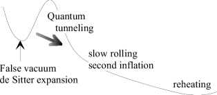
FIG. 1.: A schematic picture of the inflaton potential for a single-field model.

FIG. 2.: A schematic picture of the potential of the second inflaton field for a two-field model.

Although this model is simple, we need to assume a rather unusual form of the inflaton potential (see however [6]). To solve this problem of naturalness, models with two fields were proposed, where two different inflatons would drive the first and second stages of inflation. The first inflaton field, $\sigma$, has a double well potential. When the $\sigma$-field is in the false vacuum, the energy density of the universe is dominated by the vacuum energy of the $\sigma$-field. At this stage, the second inflaton field, $\phi$, has the potential shown by the dashed line in Fig. 2. After a sufficiently long period of inflation the $\sigma$-field makes a phase transition to the true vacuum through bubble nucleation. It is assumed that due to the coupling to the $\sigma$ field, the potential of the $\phi$-field changes into the one shown by the solid line in Fig. 2. Then, the slow roll of $\phi$ from the old minimum to the new one drives the second period of inflation in the nucleated bubble.

In some cases, the instanton describing tunneling has an approximate zero mode which can shift back and forth the value where the slow roll field lands after tunneling. In those cases, the density parameter in the resulting universe becomes a random variable, and one has an ensemble of large regions inside of each bubble where the density parameter $\Omega$ (measured at a fixed temperature) takes a range of values. This can be understood as follows.

The existence of an approximate zero mode of the instanton implies that, in the real time evolution of the bubble, there is a supercurvature mode (whose wavelength exceeds the curvature scale). Quantum excitations of this mode can change the average value of the slow roll field inside the bubble on scales larger than the Hubble radius. As a result, the amount of slow roll inflation in different regions will be different, leading to a range of values of $\Omega$ [7]. In particular, even if the instanton leads to a non-inflating value of the field after tunneling, localized fluctuations can create inflating islands which locally resemble open universes. This scenario is called “quasi-open” inflation [9, 7]. Quasi-open inflation was originally discussed in the context of two-field models, but as we shall see, models with a single field can also have supercurvature modes with similar consequences.

Finally, Hawking and Turok [10] have recently proposed that it is possible to create an open universe from nothing in a model without a false vacuum. The instanton describing this process is singular, and therefore its validity has been subject to question [11]. Nevertheless, it has also been pointed out that the quantization of linearized perturbations in the singular background is well posed [12, 13]. Therefore, provided that one can make sense of the instanton by appealing to an underlying theory where the singularity is resolved, it appears that the details of that theory need not be known in order to calculate the spectrum of cosmological perturbations.

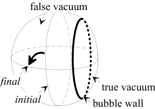
FIG. 3.: The Coleman-De Luccia instanton for the case that the spacetime dimension is two, embedded in the three dimensional Euclidean space.

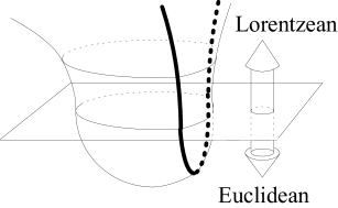
FIG. 4.: The analytic continuation of the Coleman-De Luccia instanton to the Lorentzian region. The lower half is the same as that shown in Fig.3 and represents the Euclidean region. The upper half represents the continuation to the Lorentzian region.

In order to construct an acceptable cosmological model, we must also show that the expected spectrum of primordial fluctuations is compatible with observations. Since there is an initial de Sitter expansion phase, it is natural to assume that the state before tunneling is the so-called Bunch-Davies vacuum state. Then the question that we must answer is the following: “What quantum state results after $O(4)$-symmetric bubble nucleation starting from the Euclidean vacuum state?” In the lowest order WKB approximation, the tunneling process is described by the Coleman-De Luccia bounce solution [2]. In order to extract information about the quantum fluctuations, it is necessary to develop the WKB approximation to the next order [14]. The resulting prescription to find the quantum state after tunneling can be summarized as follows.

First of all, since we shall deal with the metric perturbations which contain gauge degrees of freedom, we need to find the reduced action that contains only the physical degrees of freedom. We denote one of these degrees of freedom by $\varphi(x)$. With an appropriate choice of the variable $\varphi(x)$, the action can be reduced to that of the massive scalar field with variable mass,

$$S_{\varphi}=\int\biggl{(}-{1\over 2}g^{\mu\nu}\partial_{\mu}\varphi\partial_{\nu}\varphi-{1\over 2}{\cal M}^{2}(\eta_{C})\varphi^{2}\biggr{)}\sqrt{-g}d^{4}x.$$ (1)

From this reduced action, one can calculate expectation values following standard methods. First, we need to find a complete set of functions $v_{\bf k}$ which obey the field equation,

$$\Bigl{[}\nabla^{\mu}\nabla_{\mu}-{\cal M}^{2}(\eta_{C})\Bigr{]}v_{\bf k}(\eta,{\bf x})=0,$$ (2)

in the Lorentzian region, and which are regular on the lower hemisphere shown in Fig. 4. This restriction is due to the choice of the Bunch-Davies vacuum state before tunneling. However, the same restriction arises in the no-boundary proposal for the wave-function of the Universe [15], if Fig. 4 is interpreted as describing the creation from nothing of a universe containing a bubble. The same restriction will therefore be used in the case of the Hawking-Turok model discussed in Appendix D. Here, it is important to note that “a complete set” means a set of all modes which can be Klein-Gordon normalized on a Cauchy surface $\Sigma$ of spacetime,

$$\left\langle v_{{\bf k}}\,,v_{{\bf k}^{\prime}}\right\rangle:=-i\int_{\Sigma}d\Sigma_{\mu}g^{\mu\nu}\left\{v_{\bf k}\partial_{\nu}{\overline{v_{{\bf k}^{\prime}}}}-(\partial_{\nu}v_{{\bf k}})\overline{v_{{\bf k}^{\prime}}}\right\}=\delta_{{\bf k}{\bf k}^{\prime}}.$$ (3)

Once they are obtained, the quantum fluctuations of the field are described by the “vacuum state”, $|\Psi\rangle$, that satisfies $\hat{a}_{\bf k}|\Psi\rangle=0$ for any ${\bf k}$ where the annihilation operator $\hat{a}_{\bf k}$ is defined by the decomposition of the perturbation field:

$$\hat{\varphi}=\sum_{\bf k}(v_{\bf k}\hat{a}_{\bf k}+{\overline{v_{\bf k}}}\hat{a}_{\bf k}^{\dagger}).$$ (4)

Thus the mode functions $v_{\bf k}$ play the role of positive frequency functions.

The most tedious part in the above prescription is to find the reduced action. This is due to the fact that the time-constant hypersurface that reflects the maximal symmetry of background solution is not a Cauchy surface, and hence it is not appropriate to normalize modes. Therefore, we need to perform the reduction of the action on spacelike hypersurfaces which cut right through the bubble, and which are therefore not homogeneous. This renders the decomposition into scalar, vector and tensor modes into a rather unfamiliar form. In the end, however, the three standard physical degrees of freedom are identified [16]. When they are analytically continued to the open universe, one becomes the usual scalar-type perturbation and the other two becomes the even and odd parity tensor-type perturbations.

Along the lines of the above prescription, the prediction of the power spectrum of perturbations was given by many authors [17, 18, 20]. Until recently, however, the reduced action including the metric perturbations was not known, and for the scalar-type perturbation the studies were limited to the case in which the metric perturbation was neglected. Clearly, this should be a reasonable approximation in the weak gravity limit. Nevertheless, it turns out that the correspondence between the case where metric perturbations are neglected and the case where they are included is rather non-trivial.

In [16] we found that, at least formally, the metric perturbation has a dramatic effect on the spectrum for the scalar modes, even in the limit of weak gravitational coupling. When metric perturbations are ignored, there is a discrete wall fluctuation mode which gives a finite contribution to observables. However, when we incorporate the metric perturbation, this mode disappears. Fortunately, the contribution from the disappeared scalar-type perturbation reappears in the low frequency spectrum of even-parity tensor modes [21, 20]. In particular, we found that in the weak gravity limit the change of assignment of the wall fluctuation modes from scalar to tensor does not affect the observational quantities, such as the multipole moments of the temperature fluctuation of the cosmic microwave background. Note that the wall fluctuation mode is the Goldstone mode associated with the breakdown of spatial symmetry, and we find that it is “eaten up” by the gravitational degrees of freedom. This is reminiscent of the fate of Goldstone bosons in gauge theories.

In the present paper we shall continue the work of [16], investigating the full power spectrum of scalar perturbations. In particular, we shall consider the question of the existence of supercurvature scalar modes[18, 19]. In the previous studies in which the metric perturbation was neglected it was found that, quite generically, there are no supercurvature modes for thin wall single-field models (other than the wall fluctuation mode). It was also shown that the contribution to the CMB anisotropy due to the continuous spectrum is almost independent of the details of the potential barrier. However, it is still uncertain whether such a robust prediction of the spectrum stays correct or not when we incorporate the effect of the metric perturbation. Here we shall clarify this point. As for the tensor-type perturbations, the studies in which the perturbation of the scalar field was neglected was done in [21, 22]. Fortunately, this was found not to alter the resulting spectrum at all. However, the effect of the evolution after nucleation of a bubble has not been studied so far.

In previous studies, a simplified model was used to describe the background geometry inside the bubble, assuming that it was a pure de Sitter space. In this paper, we extend our analysis also taking into account that both the background geometry and the scalar field configuration are non-trivial.

The paper is organized as follows. In Section II we first describe the lowest WKB order picture of the bubble nucleation. After that, we briefly recall the resulting reduced action for the perturbation on this background obtained in our previous paper[16]. In Section III we consider the question of existence of scalar supercurvature modes. For this purpose, several new techniques are introduced. In particular we show that the spectra in the weak gravity limit and in the case without gravity can be related to each other using the formalism of supersymmetric quantum mechanics. We also introduce a method for reconstructing the inflaton potential barrier starting from a given bubble profile for the tunneling field. This is used to find examples which do posess supercurvature modes. In particular, we discuss an generalization of the flat space Fubini instanton [27] to de Sitter space. This example is useful in order to illustrate the role played by the scalar supercurvature modes. In Sections IV and V we consider the spectrum of the scalar-type and tensor-type perturbations, respectively. Section VI is devoted to the conclusions.

A number of issues are discussed in the appendices. In Appendix A we perform the canonical quantization of cosmological perturbations using the Dirac formalism. We recover the results of our earlier work [16], where the quantization was performed using the Fadeev-Jackiw reduction method. In Appendix B we derive some bounds on the “superpotential” which appears in the Schrödinger fluctuation operator for scalar modes. In Appendix C, we consider a class of models for which the evolution of perturbations can be solved exactly. Finally, in Appendix D we find the spectrum of cosmological perturbations in a soluble model of the Hawking-Turok type. We use the notation, $\kappa=8\pi G$, and adopt the units $c=\hbar=1$.

II reduced action for perturbations

We consider the system that consists of a minimally coupled single scalar field, $\Phi$, coupled with the Einstein gravity. We denote the potential of the field $\Phi$ by $V(\Phi)$. In order to describe the $O(4)$-symmetric bounce solution, we consider a Euclidean configuration,

$$ds^{2}=a(\eta_{E})^{2}\left[d\eta_{E}^{2}+d\chi_{E}^{2}+\sin^{2}\chi_{E}(d\theta^{2}+\sin^{2}\theta d\varphi^{2})\right],$$ (5)

$$\Phi=\phi(\eta_{E}).$$ (6)

Then, the equation of motion for the background quantities becomes

$$\phi^{\prime\prime}+2{\cal H}\phi^{\prime}-a^{2}{\partial V}=0,$$ (7)

$${\cal H}^{2}-1={\kappa\over 3}\left({1\over 2}{\phi^{\prime}}^{2}-a^{2}V(\phi)\right),$$ (8)

$${\cal H}^{\prime}-{\cal H}^{2}+1=-{\kappa\over 2}{\phi^{\prime}}^{2},$$ (9)

where the prime denotes a derivative with respect to $\eta_{E}$, ${\cal H}:=a^{\prime}/a$ and $\partial V:=dV(\phi)/d\phi$. We note that the above three equations are not independent. One of them can be derived from the other two. The bounce solution is the solution that satisfies the above set of equations with the boundary condition that $\phi^{\prime}\to 0$, $a\to 0$ and ${\cal H}\to\pm 1$ at $\eta_{E}\to\mp\infty$. The topology of the solution is the 4-sphere. Hereafter, we refer to scalar field and the scale factor of the background bounce solution by $\phi$ and $a$. The two points at which $a=0$ are the centers of the $O(4)$-symmetry. For convenience, we take $\eta_{E}=\infty$ to be on the true vacuum side (i.e., inside the $O(4)$-symmetric bubble), and call it the pole and that on the false vacuum side the antipole.

Sometimes it is convenient to use the coordinate $\tau_{E}$ defined by $d\tau_{E}=a(\eta_{E})d\eta_{E}$. In terms of it, the background equations are written as

$$\ddot{\phi}+3{\dot{a}\over a}\dot{\phi}-{\partial V}=0,$$ (10)

$$\left({\dot{a}\over a}\right)^{2}-{1\over a^{2}}={\kappa\over 3}\left({1\over 2}{\dot{\phi}}^{2}-V(\phi)\right),$$ (11)

$$\left({\dot{a}\over a}\right)^{\displaystyle\cdot}+{1\over a^{2}}=-{\kappa\over 2}{\dot{\phi}}^{2},$$ (12)

where the dot represents a derivative with respect to $\tau_{E}$.

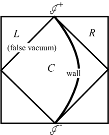
FIG. 5.: Conformal diagram of a de Sitter-like space with a bubble.

Once we know the bounce solution, the background geometry and the field configuration in the Lorentzian region are obtained by the analytic continuation of the bounce solution through the 3-sphere intersecting both poles. The coordinates in the Lorentzian region are given by

$$\eta_{E}=\eta_{C}=-\eta_{R}-{\pi\over 2}i=\eta_{L}+{\pi\over 2}i\,,$$ (13)

$$\chi_{E}=-i\chi_{C}+{\pi\over 2}=-i\chi_{L}=-i\chi_{R}\,,$$ (14)

$$a=a_{C}=ia_{R}=ia_{L}\,.$$ (15)

Accordingly, the analytic continuation of the coordinate $\tau_{E}$ is given by

$$d\tau_{E}=d\tau_{C}=-id\tau_{R}=id\tau_{L}\,.$$ (16)

The coordinates with the indices $C$, $R$ and $L$ cover regions $C$, $R$ and $L$, respectively, in Fig. 5. The region $R$ corresponds to the inside of the lightcone emanating from the center of the nucleated bubble, where $a=0$ and $\eta_{C}=\eta_{E}\to+\infty$. The region $L$ is the inside of the lightcone emanating from the antipodal point where $a=0$ and $\eta_{C}\to-\infty$. The region $C$ is the remaining central region. In region $C$, the metric is given by

$$ds^{2}=a(\eta_{C})^{2}\left[d\eta_{C}^{2}-d\chi_{C}^{2}+\cosh^{2}\chi_{C}(d\theta^{2}+\sin^{2}\theta d\varphi^{2})\right].$$ (17)

One sees that surfaces that respect the maximal symmetry, i.e., the $\eta_{C}=$const. hypersurfaces are no longer spacelike. Instead of $\eta_{C}$, the coordinate $\chi_{C}$ plays the role of the time coordinate there. Note that the $\chi_{C}=$const. hypersurfaces are not homogeneous.

In order to find the quantum state after the bubble nucleation, we need to find a set of normalized mode functions that satisfies the regularity condition explained in Introduction. As mentioned there and can be seen from Fig. 5, no Cauchy surface exists in regions $R$ and $L$. Thus, in order to obtain a set of normalized mode functions, we need to find the reduced action in region $C$, starting from the second order variation of the action including the metric perturbation on this background. This was done in our previous paper[16]. There, we used the Faddev-Jackiw method for constrained systems to obtain the reduced action. In Appendix A of this paper, as an alternative and perhaps more familiar method, we present a derivation of the reduced action a la Dirac. Perturbations on a spherical symmetric background can be decomposed into even and odd parity modes. The odd parity modes do not contribute to the CMB anisotropy if we choose the position of the observer as the center of the spherical symmetry. Hence we concentrate on even parity modes. As mentioned above, we must work in region $C$, where the background configuration is spatially inhomogeneous. However, in region $R$ or $L$, the background solution has the symmetry of the FRW universe. There the standard cosmological perturbation theory tells us that even parity perturbations for the Einstein-scalar system can be decomposed into the scalar and tensor-type perturbations. Therefore, one expects that even parity modes can be decomposed into two sets of decoupled perturbations even in region $C$ and they are naturally identified with the scalar and tensor-type perturbations, respectively, when they are analytically continued to region $R$ or $L$. This was shown to be true in [16]. Hence, following the conventional terminology used in the cosmological perturbation theory, we call the corresponding modes the scalar-type perturbation and the tensor-type perturbation, respectively, even in region $C$.

In this section, we work in region $C$ where the Cauchy surface exists. Note that we have $\eta_{E}=\eta_{C}$ and $\tau_{E}=\tau_{C}$. For notational simplicity, we omit the index $C$ from the coordinate variables throughout this section.

A Reduced action for scalar-type perturbation

First we consider the scalar-type perturbation. We introduce a gauge invariant variable $Q_{S}$ for the scalar-type perturbation which corresponds to the curvature perturbation in the Newton gauge in the open universe. Explicitly the metric and the scalar field perturbation in the Newton gauge is given as

$$ds^{2} = \left(1+{Q_{S}\over 4a}\right)d\tau^{2}+a^{2}\left(1-{Q_{S}\over 4a}\right)\left(-d\chi^{2}+\cosh^{2}\chi d\Omega^{2}\right),$$ (18)

$$\varphi_{N} = {\dot{Q}_{S}\over 4\kappa a\dot{\phi}}\,.$$ (19)

In terms of $Q_{S}$, the reduced action is obtained in Appendix A as

$$S^{(2)}_{\hbox{sca}}=\sum_{\ell,m}\int d\chi\int{d\tau\over 2a^{3}\dot{\phi}^{2}}\left[\cosh^{2}\chi{\partial\over\partial\chi}\overline{Q_{S}^{\ell m}}\widehat{K}_{S}{\partial\over\partial\chi}{Q_{S}^{\ell m}}-\overline{Q_{S}^{\ell m}}\widehat{K}_{S}\left\{{\ell(\ell+1)}+(\widehat{K}_{S}-3)\right\}{Q_{S}^{\ell m}}\right],$$ (20)

where $\ell$ and $m$ are the eigenvalues of spherical harmonic expansion, $Q_{S}^{\ell m}$ is the $(\ell,m)$-component of the spherical harmonic expansion, $Q_{S}=:\sum Q_{S}^{\ell m}Y_{\ell m}(\Omega)$, and $\widehat{K}_{S}$ is a derivative operator given by

$$\widehat{K}_{S}=\left[-a^{3}\dot{\phi}^{2}{\partial\over\partial\tau}{1\over a\dot{\phi}^{2}}{\partial\over\partial\tau}+{\kappa a^{2}\dot{\phi}^{2}\over 2}\right].$$ (21)

The relation of $Q_{S}$ to the variable $\textstyle q$ introduced in [16] is

$$Q_{S}=4\kappa a\dot{\phi}{\mathchoice{{\hbox{\boldmath$\displaystyle q$}}}{{\hbox{\boldmath$\textstyle q$}}}{{\hbox{\boldmath$\scriptstyle q$}}}{{\hbox{\boldmath$\scriptscriptstyle q$}}}}\,.$$ (22)

Putting ${\mathchoice{{\hbox{\boldmath$\displaystyle q$}}}{{\hbox{\boldmath$\textstyle q$}}}{{\hbox{\boldmath$\scriptstyle q$}}}{{\hbox{\boldmath$\scriptscriptstyle q$}}}}=\sum{\mathchoice{{\hbox{\boldmath$\displaystyle q$}}}{{\hbox{\boldmath$\textstyle q$}}}{{\hbox{\boldmath$\scriptstyle q$}}}{{\hbox{\boldmath$\scriptscriptstyle q$}}}}^{\ell m}Y_{\ell m}$, we can use this relation to rewrite the reduced action (20) into the form,

$$S^{(2)}_{\hbox{sca}}=\sum_{\ell,m}{1\over 2}\int d\chi\int{d\eta}\left[\cosh^{2}\chi{\partial\overline{{\mathchoice{{\hbox{\boldmath$\displaystyle q$}}}{{\hbox{\boldmath$\textstyle q$}}}{{\hbox{\boldmath$\scriptstyle q$}}}{{\hbox{\boldmath$\scriptscriptstyle q$}}}}^{\ell m}}\over\partial\chi}\widehat{\cal O}{\partial{\mathchoice{{\hbox{\boldmath$\displaystyle q$}}}{{\hbox{\boldmath$\textstyle q$}}}{{\hbox{\boldmath$\scriptstyle q$}}}{{\hbox{\boldmath$\scriptscriptstyle q$}}}}^{\ell m}\over\partial\chi}-\overline{{\mathchoice{{\hbox{\boldmath$\displaystyle q$}}}{{\hbox{\boldmath$\textstyle q$}}}{{\hbox{\boldmath$\scriptstyle q$}}}{{\hbox{\boldmath$\scriptscriptstyle q$}}}}^{\ell m}}\widehat{\cal O}\left\{{\ell(\ell+1)}+(\widehat{\cal O}-3)\cosh^{2}\chi\right\}{\mathchoice{{\hbox{\boldmath$\displaystyle q$}}}{{\hbox{\boldmath$\textstyle q$}}}{{\hbox{\boldmath$\scriptstyle q$}}}{{\hbox{\boldmath$\scriptscriptstyle q$}}}}^{\ell m}\right],$$ (23)

where the operator $\widehat{\cal O}$ is given by

$$\widehat{\cal O}=-{d^{2}\over d\eta^{2}}+{\kappa\over 2}{\phi^{\prime}}^{2}+\phi^{\prime}\left({1\over\phi^{\prime}}\right)^{\prime\prime}.$$ (24)

The reduced action (23) exactly coincides with the one derived in [16]. Notice that in terms of $Q_{S}$ the action contains the operator $\widehat{K}_{S}$, which is not Schrödinger-like, whereas in terms of $\textstyle q$ it contains the operator $\widehat{\cal O}$, which is. Although this is of no essential significance, the second form is more convenient when normalizing the modes and when discussing the general form of the primordial spectrum.

Now let us construct a set of positive frequency functions corresponding to the variable $\textstyle q$. It is decomposed as

$${{\mathchoice{{\hbox{\boldmath$\displaystyle q$}}}{{\hbox{\boldmath$\textstyle q$}}}{{\hbox{\boldmath$\scriptstyle q$}}}{{\hbox{\boldmath$\scriptscriptstyle q$}}}}}^{\ell m}=\sum{\cal N}^{S}_{p}{\mathchoice{{\hbox{\boldmath$\displaystyle q$}}}{{\hbox{\boldmath$\textstyle q$}}}{{\hbox{\boldmath$\scriptstyle q$}}}{{\hbox{\boldmath$\scriptscriptstyle q$}}}}^{p}(\eta)f^{p\ell}(\chi),$$ (25)

where ${\cal N}_{p}^{S}$ is a normalization constant, and the sum is understood as a sum over the discrete spectra and as an integral over the continuum one. In this expression, ${\mathchoice{{\hbox{\boldmath$\displaystyle q$}}}{{\hbox{\boldmath$\textstyle q$}}}{{\hbox{\boldmath$\scriptstyle q$}}}{{\hbox{\boldmath$\scriptscriptstyle q$}}}}^{p}(\eta)$ is a spatial eigenfunction of the operator $\widehat{\cal O}$ with the eigenvalue $p^{2}+4$. That is, ${\mathchoice{{\hbox{\boldmath$\displaystyle q$}}}{{\hbox{\boldmath$\textstyle q$}}}{{\hbox{\boldmath$\scriptstyle q$}}}{{\hbox{\boldmath$\scriptscriptstyle q$}}}}^{p}(\eta)$ satisfies

$$\widehat{\cal O}{{\mathchoice{{\hbox{\boldmath$\displaystyle q$}}}{{\hbox{\boldmath$\textstyle q$}}}{{\hbox{\boldmath$\scriptstyle q$}}}{{\hbox{\boldmath$\scriptscriptstyle q$}}}}}^{p}=\left[-{d^{2}\over d\eta^{2}}+{\kappa\over 2}{\phi^{\prime}}^{2}+\phi^{\prime}\left({1\over\phi^{\prime}}\right)^{\prime\prime}\right]{{\mathchoice{{\hbox{\boldmath$\displaystyle q$}}}{{\hbox{\boldmath$\textstyle q$}}}{{\hbox{\boldmath$\scriptstyle q$}}}{{\hbox{\boldmath$\scriptscriptstyle q$}}}}}^{p}=(p^{2}+4){{\mathchoice{{\hbox{\boldmath$\displaystyle q$}}}{{\hbox{\boldmath$\textstyle q$}}}{{\hbox{\boldmath$\scriptstyle q$}}}{{\hbox{\boldmath$\scriptscriptstyle q$}}}}}^{p}.$$ (26)

The equation that determines the time evolution is found to be model independent and becomes

$$\left[-{1\over\cosh^{2}\chi}{\partial\over\partial\chi}\cosh^{2}\chi{\partial\over\partial\chi}-{\ell(\ell+1)\over\cosh^{2}\chi}\right]f^{p\ell}=(p^{2}+1)f^{p\ell}.$$ (27)

Aside from the normalization factor, the positive frequency function is determined by the Bunch-Davies regularity condition, namely, it must be regular at $\chi=0$ ($\chi_{E}=\pi/2$). The solution is

$$f^{p\ell}(\chi)=\sqrt{{\Gamma(ip+\ell+1)\Gamma(-ip+\ell+1)\over\Gamma(ip)\Gamma(-ip)\cosh\chi}}P^{-\ell-1/2}_{ip-1/2}(i\sinh\chi),$$ (28)

where $P^{\mu}_{\nu}$ is the associated Legendre function of the first kind, and we have fixed the normalization factor so that the analytic continuation of $Y^{p\ell m}(\chi,\Omega):=f^{pl}(\chi)Y_{\ell m}(\Omega)$ to region $R$ or $L$ satisfies

$$\int\sinh^{2}\chi\,d\chi\,d\Omega\,Y^{p\ell m}\overline{Y^{p^{\prime}\ell^{\prime}m^{\prime}}}=\delta(p-p^{\prime})\delta_{\ell\ell^{\prime}}\delta_{mm^{\prime}},$$ (29)

for $p^{2}>0$, where $\chi=\chi_{R}$ or $\chi_{L}$. Also, these analytically continued harmonics satisfy

$${}^{(3)}\Delta\,Y^{p\ell m}=-(p^{2}+1)Y^{p\ell m},$$ (30)

where ${}^{(3)}\Delta$ is the Laplacian on the unit spacelike hyperboloid. For $p^{2}<0$, the normalization factor in Eq. (28) is not suitable. In this case, the solutions to (27) will be denoted by $f^{\Lambda,\ell}(\chi)$, where $\Lambda^{2}=-p^{2}$. The positive frequency functions $f^{\Lambda,\ell}(\chi)$ are taken as the usual Bunch-Davies ones,

$$f^{\Lambda,\ell}(\chi)=\sqrt{{\Gamma(\Lambda+\ell+1)\Gamma(-\Lambda+\ell+1)\over 2\cosh\chi}}P^{-\ell-1/2}_{\Lambda-1/2}(i\sinh\chi),$$ (31)

and we define ${\cal Y}^{\Lambda,\ell m}(\chi,\Omega):=f^{\Lambda,\ell}(\chi)Y_{\ell m}(\Omega)$. Notice that with this choice of positive frequency functions, ${\cal Y}^{\Lambda,\ell m}$ are already Klein-Gordon normalized in the (2+1) dimensional sense, i.e.

$$i\cosh^{2}\chi\left\{{\partial f^{\Lambda,\ell}\over\partial\chi}\overline{f^{\Lambda,\ell}}-f^{\Lambda,\ell}{\partial\overline{f^{\Lambda,\ell}}\over\partial\chi}\right\}\int d\Omega\,Y_{\ell m}\overline{Y_{\ell^{\prime}m^{\prime}}}=\delta_{\ell\ell^{\prime}}\delta_{mm^{\prime}}\,.$$ (32)

These mode functions ${\cal Y}^{\Lambda,\ell m}$ also satisfy Eq. (30) in region R.

In order to quantize the perturbations, it is convenient to write the action (20) in the canonical form (1). Introducing a new variable $\check{\mathchoice{{\hbox{\boldmath$\displaystyle q$}}}{{\hbox{\boldmath$\textstyle q$}}}{{\hbox{\boldmath$\scriptstyle q$}}}{{\hbox{\boldmath$\scriptscriptstyle q$}}}}:=\sum\sqrt{p^{2}+4}\,a^{-1}{\cal N}^{S}_{p}{\mathchoice{{\hbox{\boldmath$\displaystyle q$}}}{{\hbox{\boldmath$\textstyle q$}}}{{\hbox{\boldmath$\scriptstyle q$}}}{{\hbox{\boldmath$\scriptscriptstyle q$}}}}^{p}(\eta)Y^{p\ell m}(\chi,\Omega)+\sum\sqrt{4-\Lambda^{2}}\,a^{-1}{\cal N}^{S}_{,\Lambda}{\mathchoice{{\hbox{\boldmath$\displaystyle q$}}}{{\hbox{\boldmath$\textstyle q$}}}{{\hbox{\boldmath$\scriptstyle q$}}}{{\hbox{\boldmath$\scriptscriptstyle q$}}}}^{,\Lambda}(\eta){\cal Y}^{\Lambda,\ell m}(\chi,\Omega)$, the action for $\check{\mathchoice{{\hbox{\boldmath$\displaystyle q$}}}{{\hbox{\boldmath$\textstyle q$}}}{{\hbox{\boldmath$\scriptstyle q$}}}{{\hbox{\boldmath$\scriptscriptstyle q$}}}}$ turns out to be the one for a scalar field with $\eta$-dependent mass. Thus the normalized positive frequency functions are determined by calculating the ordinary Klein-Gordon norm for $\check{\mathchoice{{\hbox{\boldmath$\displaystyle q$}}}{{\hbox{\boldmath$\textstyle q$}}}{{\hbox{\boldmath$\scriptstyle q$}}}{{\hbox{\boldmath$\scriptscriptstyle q$}}}}$. Namely we require

$$i({p^{2}+4})\cosh^{2}\chi|{\cal N}_{p}^{S}|^{2}\left\{{\partial f^{pl}\over\partial\chi}\overline{f^{pl}}-f^{pl}{\partial\overline{f^{pl}}\over\partial\chi}\right\}\int_{-\infty}^{\infty}d\eta\,{\mathchoice{{\hbox{\boldmath$\displaystyle q$}}}{{\hbox{\boldmath$\textstyle q$}}}{{\hbox{\boldmath$\scriptstyle q$}}}{{\hbox{\boldmath$\scriptscriptstyle q$}}}}^{p}\overline{{\mathchoice{{\hbox{\boldmath$\displaystyle q$}}}{{\hbox{\boldmath$\textstyle q$}}}{{\hbox{\boldmath$\scriptstyle q$}}}{{\hbox{\boldmath$\scriptscriptstyle q$}}}}^{p^{\prime}}}$$ (33)

$$\quad={2p(p^{2}+4)\sinh\pi p\,|{\cal N}_{p}^{S}|^{2}\over\pi}\int_{-\infty}^{\infty}d\eta\,{\mathchoice{{\hbox{\boldmath$\displaystyle q$}}}{{\hbox{\boldmath$\textstyle q$}}}{{\hbox{\boldmath$\scriptstyle q$}}}{{\hbox{\boldmath$\scriptscriptstyle q$}}}}^{p}\overline{{\mathchoice{{\hbox{\boldmath$\displaystyle q$}}}{{\hbox{\boldmath$\textstyle q$}}}{{\hbox{\boldmath$\scriptstyle q$}}}{{\hbox{\boldmath$\scriptscriptstyle q$}}}}^{p^{\prime}}}=\delta(p-p^{\prime})$$ (34)

for the continuous spectrum ($p^{2}>0$), and

$$({4-\Lambda^{2}})|{\cal N}_{,\Lambda}^{S}|^{2}\int_{-\infty}^{\infty}d\eta\,{\mathchoice{{\hbox{\boldmath$\displaystyle q$}}}{{\hbox{\boldmath$\textstyle q$}}}{{\hbox{\boldmath$\scriptstyle q$}}}{{\hbox{\boldmath$\scriptscriptstyle q$}}}}^{,\Lambda}\overline{{\mathchoice{{\hbox{\boldmath$\displaystyle q$}}}{{\hbox{\boldmath$\textstyle q$}}}{{\hbox{\boldmath$\scriptstyle q$}}}{{\hbox{\boldmath$\scriptscriptstyle q$}}}}^{,\Lambda^{\prime}}}=\delta_{\Lambda\Lambda^{\prime}},$$ (35)

for the discrete one ($p^{2}<0$). Notice that the Klein-Gordon normalization reduces to a Schrödinger-like normalization for ${\mathchoice{{\hbox{\boldmath$\displaystyle q$}}}{{\hbox{\boldmath$\textstyle q$}}}{{\hbox{\boldmath$\scriptstyle q$}}}{{\hbox{\boldmath$\scriptscriptstyle q$}}}}_{p}$ (once a convenient choice of ${\cal N}_{p}^{S}$ has been made)

The variable $Q_{S}$ can be also decomposed in the same way as $\textstyle q$. From Eq. (22), the corresponding spatial eigenfunction $Q_{S}^{p}(\tau)$ is related to ${\mathchoice{{\hbox{\boldmath$\displaystyle q$}}}{{\hbox{\boldmath$\textstyle q$}}}{{\hbox{\boldmath$\scriptstyle q$}}}{{\hbox{\boldmath$\scriptscriptstyle q$}}}}^{p}(\tau)$ as $Q_{S}^{p}=\sqrt{\kappa}\,a\dot{\phi}\,{\mathchoice{{\hbox{\boldmath$\displaystyle q$}}}{{\hbox{\boldmath$\textstyle q$}}}{{\hbox{\boldmath$\scriptstyle q$}}}{{\hbox{\boldmath$\scriptscriptstyle q$}}}}^{p}$. The equation satisfied by $Q_{S}^{p}$ is given by the eigenvalue equation for the operator $\widehat{K}_{S}$ as

$$a^{-2}\widehat{K}_{S}Q_{S}^{p}=\left(-a\dot{\phi}^{2}{d\over d\tau}{1\over a\dot{\phi}^{2}}{d\over d\tau}+{\kappa\over 2}\dot{\phi}^{2}\right){Q_{S}^{p}}={p^{2}+4\over a^{2}}Q_{S}^{p}.$$ (36)

For later convenience, we also write down the equation for the scalar field fluctuation in the Newton gauge:

$$\ddot{\varphi}_{N}^{p}+3{\dot{a}\over a}\dot{\varphi}_{N}^{p}+\left({p^{2}+1\over a^{2}}-\partial^{2}V\right)\varphi_{N}^{p}=2\kappa\dot{\phi}^{2}\varphi_{N}^{p}+{d\over d\tau}(a\dot{\phi})\,{Q_{S}^{p}\over 4a^{2}}\,,$$ (37)

where $\partial^{2}V:=d^{2}V/d\phi^{2}$ and $\varphi_{N}$ has been expanded in the same way as $\textstyle q$. We note that from the Newton gauge condition (A61) in Appendix A, we have

$$\dot{Q}_{S}^{p}=4\kappa a\dot{\phi}\varphi_{N}^{p}=4\kappa{d\over d\tau}(a\dot{\phi}\,{\mathchoice{{\hbox{\boldmath$\displaystyle q$}}}{{\hbox{\boldmath$\textstyle q$}}}{{\hbox{\boldmath$\scriptstyle q$}}}{{\hbox{\boldmath$\scriptscriptstyle q$}}}}^{p}).$$ (38)

Using this, Eq. (37) may be rewritten as

$$\ddot{\varphi}_{N}^{p}+3{\dot{a}\over a}\dot{\varphi}_{N}^{p}\left({p^{2}+1\over a^{2}}-\partial^{2}V\right)\varphi_{N}^{p}=3\kappa\dot{\phi}^{2}\varphi_{N}^{p}-\kappa\dot{\phi}^{2}\dot{\mathchoice{{\hbox{\boldmath$\displaystyle q$}}}{{\hbox{\boldmath$\textstyle q$}}}{{\hbox{\boldmath$\scriptstyle q$}}}{{\hbox{\boldmath$\scriptscriptstyle q$}}}}^{p}.$$ (39)

The analytic continuation of the variables $Q_{S}$, $\varphi_{N}$ and $\textstyle q$ to region $R$ or $L$ is given by

$$Q_{S}^{C}=iQ_{S}^{R}=iQ_{S}^{L},\quad\varphi_{N}^{C}=\varphi_{N}^{R}=\varphi_{N}^{L},\quad{{\mathchoice{{\hbox{\boldmath$\displaystyle q$}}}{{\hbox{\boldmath$\textstyle q$}}}{{\hbox{\boldmath$\scriptstyle q$}}}{{\hbox{\boldmath$\scriptscriptstyle q$}}}}}_{C}=-i{{\mathchoice{{\hbox{\boldmath$\displaystyle q$}}}{{\hbox{\boldmath$\textstyle q$}}}{{\hbox{\boldmath$\scriptstyle q$}}}{{\hbox{\boldmath$\scriptscriptstyle q$}}}}}_{R}=i{\mathchoice{{\hbox{\boldmath$\displaystyle q$}}}{{\hbox{\boldmath$\textstyle q$}}}{{\hbox{\boldmath$\scriptstyle q$}}}{{\hbox{\boldmath$\scriptscriptstyle q$}}}}_{L},$$ (40)

where the indices $C$, $L$ and $R$ denote the variables in the respective regions. The evolution equation in an open universe inside the bubble is given by the analytic continuation of Eq. (26), or Eq. (39) supplemented by Eq. (38). We note that the form of the equations does not change after the analytic continuation except for the signature in front of $\partial^{2}V$ in Eq. (39).

B Reduced action for tensor-type perturbation

In this subsection, we consider the tensor-type perturbation. We introduce a gauge invariant variable $Q_{T}$ that corresponds to the tensor-type perturbation in the transverse-traceless gauge in the open universe. Let us denote the metric on a unit 2-sphere by $d\Omega^{2}=\hat{\sigma}_{AB}d\sigma^{A}d\sigma^{B}$, and the covariant derivative and the Laplacian with respect to $\hat{\sigma}_{AB}$ by ${}^{(2)}\nabla$ and ${}^{(2)}\Delta$, respectively. The tensor-type perturbation is expressed as

$$ds^{2} = d\tau^{2}-\left(a^{2}-{2Q_{T}\over\cosh^{2}\chi}\right)d\chi^{2}+\left(a^{2}+{Q_{T}\over\cosh^{2}\chi}\right)\cosh^{2}\chi\,d\Omega^{2}$$ (44)

$$+4\left(\partial_{\chi}+\tanh\chi\right){}^{(2)}\nabla_{A}({}^{(2)}\Delta)^{-1}Q_{T}\,d\chi\,d\sigma^{A}$$

$$+4\cosh^{2}\chi\left(2-\widehat{K}_{T}+{({}^{(2)}\Delta)-2\over 2\cosh^{2}\chi}+\tanh\chi\partial_{\chi}\right)$$

$$\quad\times\left[{}^{(2)}\nabla_{A}{}^{(2)}\nabla_{B}-{1\over 2}\hat{\sigma}_{AB}{}^{(2)}\Delta\right]({}^{(2)}\Delta({}^{(2)}\Delta+2))^{-1}Q_{T}d\sigma^{A}d\sigma^{B},$$

$$=: ds^{2}_{(0)}+a^{2}\,{\mathchoice{{\hbox{\boldmath$\displaystyle h$}}}{{\hbox{\boldmath$\textstyle h$}}}{{\hbox{\boldmath$\scriptstyle h$}}}{{\hbox{\boldmath$\scriptscriptstyle h$}}}}_{ij}[Q_{T}]dx^{i}dx^{j},$$ (45)

where $i,\,j=\chi,\,\theta,\,\varphi$ and

$$\widehat{K}_{T}=\left[-a{\partial\over\partial\tau}a^{3}{\partial\over\partial\tau}{1\over a^{2}}\right].$$ (46)

The action for $Q_{T}$ is obtained in Appendix A and it is given by

$$S^{(2)}_{\hbox{GW}}=\sum_{\ell,m}{2\over\kappa(\ell-1)\ell(\ell+1)(\ell+2)}\int d\chi\int{d\tau\over 2a^{3}} \Biggl{[}\cosh^{2}\chi{\partial\over\partial\chi}\overline{Q_{T}^{\ell m}}{\widehat{K}_{T}(\widehat{K}_{T}-1)}{\partial\over\partial\chi}{Q_{T}^{\ell m}}$$ (48)

$$-\overline{Q_{T}^{\ell m}}\widehat{K}_{T}(\widehat{K}_{T}-1)\left\{{\ell(\ell+1)}+\widehat{K}_{T}\cosh^{2}\chi\right\}{Q_{T}^{\ell m}}\Biggr{]},$$

where $Q_{T}^{\ell m}$ is defined by $Q_{T}=:\sum Q_{T}^{\ell m}Y_{\ell m}$, as before.

Again, the operator $\widehat{K}_{T}$ is not of Schrodinger type. Therefore, it is convenient to change to the variable $\textstyle w$ introduced in [16], which is related to $Q_{T}$ by

$$\mathchoice{{\hbox{\boldmath$\displaystyle w$}}}{{\hbox{\boldmath$\textstyle w$}}}{{\hbox{\boldmath$\scriptstyle w$}}}{{\hbox{\boldmath$\scriptscriptstyle w$}}}={a^{2}\over\kappa}{\partial\over\partial\tau}{Q_{T}\over a^{2}}.$$ (49)

Using this relation, the reduced action (48) can be rewritten as

$$S_{\hbox{GW}}^{(2)}=\sum_{\ell,m}{\kappa\over(\ell-1)\ell(\ell+1)(\ell+2)}\int d\chi\int{d\eta} \Biggl{[}\cosh^{2}\chi{\partial\overline{\mathchoice{{\hbox{\boldmath$\displaystyle w$}}}{{\hbox{\boldmath$\textstyle w$}}}{{\hbox{\boldmath$\scriptstyle w$}}}{{\hbox{\boldmath$\scriptscriptstyle w$}}}^{\ell m}}\over\partial\chi}\widehat{K}{\partial\mathchoice{{\hbox{\boldmath$\displaystyle w$}}}{{\hbox{\boldmath$\textstyle w$}}}{{\hbox{\boldmath$\scriptstyle w$}}}{{\hbox{\boldmath$\scriptscriptstyle w$}}}^{\ell m}\over\partial\chi}$$ (51)

$$-\overline{\mathchoice{{\hbox{\boldmath$\displaystyle w$}}}{{\hbox{\boldmath$\textstyle w$}}}{{\hbox{\boldmath$\scriptstyle w$}}}{{\hbox{\boldmath$\scriptscriptstyle w$}}}^{\ell m}}\widehat{K}\left\{{\ell(\ell+1)}+(\widehat{K}+1)\cosh^{2}\chi\right\}\mathchoice{{\hbox{\boldmath$\displaystyle w$}}}{{\hbox{\boldmath$\textstyle w$}}}{{\hbox{\boldmath$\scriptstyle w$}}}{{\hbox{\boldmath$\scriptscriptstyle w$}}}^{\ell m}\Biggr{]},$$

where the operator ${\widehat{K}}$ is given by

$${\widehat{K}}=-\frac{\partial^{2}}{\partial\eta^{2}}+\frac{\kappa}{2}{\phi^{\prime}}^{2}.$$ (52)

This coincides with the reduced action obtained in [16].

Now we construct a set of positive frequency functions. First we use the variable $\textstyle w$. As before, we decompose $\textstyle w$ as

$${\mathchoice{{\hbox{\boldmath$\displaystyle w$}}}{{\hbox{\boldmath$\textstyle w$}}}{{\hbox{\boldmath$\scriptstyle w$}}}{{\hbox{\boldmath$\scriptscriptstyle w$}}}}=\sum{\mathchoice{{\hbox{\boldmath$\displaystyle w$}}}{{\hbox{\boldmath$\textstyle w$}}}{{\hbox{\boldmath$\scriptstyle w$}}}{{\hbox{\boldmath$\scriptscriptstyle w$}}}}^{\ell m}Y_{\ell m}\,,\quad{{\mathchoice{{\hbox{\boldmath$\displaystyle w$}}}{{\hbox{\boldmath$\textstyle w$}}}{{\hbox{\boldmath$\scriptstyle w$}}}{{\hbox{\boldmath$\scriptscriptstyle w$}}}}}^{\ell m}=\sum{\cal N}^{T}_{p\ell}{\mathchoice{{\hbox{\boldmath$\displaystyle w$}}}{{\hbox{\boldmath$\textstyle w$}}}{{\hbox{\boldmath$\scriptstyle w$}}}{{\hbox{\boldmath$\scriptscriptstyle w$}}}}^{p}(\eta)f^{p\ell}(\chi).$$ (53)

Note that the time-dependent part, $f^{p\ell}(\chi)$, is the same as in the scalar-type perturbation. In this expression, the spatial function ${\mathchoice{{\hbox{\boldmath$\displaystyle w$}}}{{\hbox{\boldmath$\textstyle w$}}}{{\hbox{\boldmath$\scriptstyle w$}}}{{\hbox{\boldmath$\scriptscriptstyle w$}}}}^{p}(\eta)$ satisfies the eigenvalue equation for the operator $\widehat{K}$ with the eigenvalue $p^{2}$:

$${\widehat{K}}{\mathchoice{{\hbox{\boldmath$\displaystyle w$}}}{{\hbox{\boldmath$\textstyle w$}}}{{\hbox{\boldmath$\scriptstyle w$}}}{{\hbox{\boldmath$\scriptscriptstyle w$}}}}^{p}=\left[-{d^{2}\over d\eta^{2}}+{\kappa\over 2}{\phi^{\prime}}^{2}\right]{{\mathchoice{{\hbox{\boldmath$\displaystyle w$}}}{{\hbox{\boldmath$\textstyle w$}}}{{\hbox{\boldmath$\scriptstyle w$}}}{{\hbox{\boldmath$\scriptscriptstyle w$}}}}}^{p}=p^{2}{{\mathchoice{{\hbox{\boldmath$\displaystyle w$}}}{{\hbox{\boldmath$\textstyle w$}}}{{\hbox{\boldmath$\scriptstyle w$}}}{{\hbox{\boldmath$\scriptscriptstyle w$}}}}}^{p}.$$ (54)

It is important to note that the spectrum of $p$ is continuous with $p^{2}>0$ because the potential term ${\kappa\over 2}{\phi^{\prime}}^{2}$ is positive definite and vanishes at infinity. Then, defining a new variable $\check{\mathchoice{{\hbox{\boldmath$\displaystyle w$}}}{{\hbox{\boldmath$\textstyle w$}}}{{\hbox{\boldmath$\scriptstyle w$}}}{{\hbox{\boldmath$\scriptscriptstyle w$}}}}:=\sum\sqrt{2\kappa p^{2}\over(\ell-1)\ell(\ell+1)(\ell+2)}\,a^{-1}{\cal N}_{p\ell}^{T}{\mathchoice{{\hbox{\boldmath$\displaystyle w$}}}{{\hbox{\boldmath$\textstyle w$}}}{{\hbox{\boldmath$\scriptstyle w$}}}{{\hbox{\boldmath$\scriptscriptstyle w$}}}}^{p}(\eta)Y^{p\ell m}(\chi,\Omega)$, the action reduces to the one for a scalar field, as in the case of scalar-type perturbation. Therefore, the normalization condition becomes

$${2\kappa p^{2}\over(\ell-1)\ell(\ell+1)(\ell+2)}{2p\sinh\pi p\,|{\cal N}_{p\ell}^{T}|^{2}\over\pi}\int_{-\infty}^{\infty}d\eta\,{\mathchoice{{\hbox{\boldmath$\displaystyle w$}}}{{\hbox{\boldmath$\textstyle w$}}}{{\hbox{\boldmath$\scriptstyle w$}}}{{\hbox{\boldmath$\scriptscriptstyle w$}}}}^{p}\overline{{\mathchoice{{\hbox{\boldmath$\displaystyle w$}}}{{\hbox{\boldmath$\textstyle w$}}}{{\hbox{\boldmath$\scriptstyle w$}}}{{\hbox{\boldmath$\scriptscriptstyle w$}}}}^{p^{\prime}}}=\delta(p-p^{\prime}).$$ (55)

Since what we are interested in is the metric perturbation, we now consider $Q_{T}$. It can be also decomposed as ${Q_{T}}=\sum{\cal N}_{p\ell}^{T}{Q_{T}}^{p}(\tau)Y^{p\ell m}(\chi,\Omega)$, where the spatial function $Q_{T}^{p}$ satisfies the eigenvalue equation for the operator $\widehat{K}_{T}$:

$$\widehat{K}_{T}{Q_{T}^{p}}=-a^{4}\left[{d^{2}\over d\tau^{2}}+3{\dot{a}\over a}{d\over d\tau}\right]{Q_{T}^{p}\over a^{2}}=(p^{2}+1)Q_{T}^{p}\,.$$ (56)

Then the metric perturbation ${\mathchoice{{\hbox{\boldmath$\displaystyle h$}}}{{\hbox{\boldmath$\textstyle h$}}}{{\hbox{\boldmath$\scriptstyle h$}}}{{\hbox{\boldmath$\scriptscriptstyle h$}}}}_{ij}[Q_{T}]$ is given by

$${\mathchoice{{\hbox{\boldmath$\displaystyle h$}}}{{\hbox{\boldmath$\textstyle h$}}}{{\hbox{\boldmath$\scriptstyle h$}}}{{\hbox{\boldmath$\scriptscriptstyle h$}}}}_{ij}[Q_{T}]=2\sum\sqrt{2p^{2}(p^{2}+1)\over(\ell-1)\ell(\ell+1)(\ell+2)}\,{\cal N}_{p\ell}^{T}\frac{Q_{T}^{p}}{a^{2}}Y_{ij}^{(+)p\ell m},$$ (57)

where

$$Y_{ij}^{(+)p\ell m}:={1\over 2}\sqrt{(\ell-1)\ell(\ell+1)(\ell+2)\over 2p^{2}(p^{2}+1)}\,a^{2}\,{\mathchoice{{\hbox{\boldmath$\displaystyle h$}}}{{\hbox{\boldmath$\textstyle h$}}}{{\hbox{\boldmath$\scriptstyle h$}}}{{\hbox{\boldmath$\scriptscriptstyle h$}}}}_{ij}[Y^{p\ell m}].$$ (58)

The tensor $Y_{ij}^{(+)p\ell m}$ is defined so that its analytic continuation to region $R$ or $L$ gives the normalized even parity tensor harmonics on the unit 3-hyperboloid [23], i.e.,

$$\int d^{3}x\sqrt{\hat{\gamma}}\,\hat{\gamma}^{ii^{\prime}}\hat{\gamma}^{jj^{\prime}}Y^{(+)p\ell m}_{ij}\overline{Y^{p^{\prime}\ell^{\prime}m^{\prime}}_{i^{\prime}j^{\prime}}}=\delta(p-p^{\prime})\delta_{\ell\ell^{\prime}}\delta_{mm^{\prime}}\,,$$ (59)

where $\hat{\gamma}_{ij}$ is the metric on the unit 3-hyperboloid and $\hat{\gamma}=\det\hat{\gamma}_{ij}$. Therefore it is more relevant to introduce a new normalization constant for the tensor perturbation:

$$\tilde{\cal N}_{p}^{T}:=2\sqrt{2p^{2}(p^{2}+1)\over(\ell-1)\ell(\ell+1)(\ell+2)}\,{\cal N}_{p\ell}^{T}\,,$$ (60)

with which the metric perturbation is expressed as

$${\mathchoice{{\hbox{\boldmath$\displaystyle h$}}}{{\hbox{\boldmath$\textstyle h$}}}{{\hbox{\boldmath$\scriptstyle h$}}}{{\hbox{\boldmath$\scriptscriptstyle h$}}}}_{ij}[Q_{T}]=\sum\tilde{\cal N}_{p}^{T}\frac{Q_{T}^{p}}{a^{2}}Y_{ij}^{(+)p\ell m}.$$ (61)

In terms of $\tilde{\cal N}_{p}^{T}$, the normalization condition (55) is re-expressed as

$${\kappa p\sinh\pi p|\tilde{\cal N}_{p}^{T}|^{2}\over 2\pi(p^{2}+1)}\left[\int_{-\infty}^{\infty}d\eta{\mathchoice{{\hbox{\boldmath$\displaystyle w$}}}{{\hbox{\boldmath$\textstyle w$}}}{{\hbox{\boldmath$\scriptstyle w$}}}{{\hbox{\boldmath$\scriptscriptstyle w$}}}}^{p}\overline{{\mathchoice{{\hbox{\boldmath$\displaystyle w$}}}{{\hbox{\boldmath$\textstyle w$}}}{{\hbox{\boldmath$\scriptstyle w$}}}{{\hbox{\boldmath$\scriptscriptstyle w$}}}}^{p^{\prime}}}\right]=\delta(p-p^{\prime}).$$ (62)

The relations between the analytically continued variables are given by

$$Q_{T}^{C}=Q_{T}^{R}=Q_{T}^{L},\quad{\mathchoice{{\hbox{\boldmath$\displaystyle w$}}}{{\hbox{\boldmath$\textstyle w$}}}{{\hbox{\boldmath$\scriptstyle w$}}}{{\hbox{\boldmath$\scriptscriptstyle w$}}}}_{C}=i{\mathchoice{{\hbox{\boldmath$\displaystyle w$}}}{{\hbox{\boldmath$\textstyle w$}}}{{\hbox{\boldmath$\scriptstyle w$}}}{{\hbox{\boldmath$\scriptscriptstyle w$}}}}_{R}=-i{\mathchoice{{\hbox{\boldmath$\displaystyle w$}}}{{\hbox{\boldmath$\textstyle w$}}}{{\hbox{\boldmath$\scriptstyle w$}}}{{\hbox{\boldmath$\scriptscriptstyle w$}}}}_{L}.$$ (63)

III scalar supercurvature modes

The possible presence of scalar supercurvature modes (i.e. modes with $p^{2}<0$) has important physical consequences. If a model has supercurvature scalar modes then the density parameter $\Omega$ becomes a random variable which takes different values in different places of the universe, and as we shall see, it may have a considerable spread if $p^{2}$ is close to $-1$ [9, 7]. Also, if the spectrum of perturbations around a particular bubble contains a “supercritical” eigenvalue with $p^{2}<-1$, this may indicate that we are not looking at the dominant channel for decay, and that there is another instanton with a lower Euclidean action (This is known as the “no supercritical supercurvature” mode conjecture which has been shown to hold in several cases [24]). In this section we shall analyze the conditions for the existence of scalar supercurvature modes in one field models of open inflation. We conclude that generically, these will be absent in the thin wall case, although they can be present for thick wall models (and even for thin wall models with sufficiently complicated potentials.) Intuitively, the reason is that for thin wall models the microphysical mass scales are large compared with the inverse size of the bubble, and hence all modes of fluctuation are “hard”. In contrast, two-field models generically have supercurvature modes [18] even in the thin wall case. These are not due to the tunneling field but to the “soft” modes of the slow roll inflaton field - roughly speaking, the value of the slow roll field at the time of nucleation may be seen as an approximate zero mode of the action.

First of all, in subsection III A we shall investigate the weak gravity limit, comparing the scalar spectrum in the case when metric perturbations are included and the case when they are neglected. The formalism of supersymmetric quantum mechanics turns out to be very useful in this respect. Then, in subsection III B we shall give a sufficient condition for the existence of scalar supercurvature modes. In subsection III C, we describe a method to construct a model which has supercurvature modes when the bubble wall is thick but does not have them when the bubble wall is thin. In subsection III D we consider the generalization of the Fubini instanton to a de Sitter background and use it to illustrate the role played by supercurvature modes in one field models.

A Supersymmetric Quantum Mechanics and the weak gravity limit

For scalar perturbations the spectrum is determined by the Schrödinger operator $\widehat{\cal O}$ in Eq. (26). This can be rewritten in the form

$$\widehat{\cal O}{\mathchoice{{\hbox{\boldmath$\displaystyle q$}}}{{\hbox{\boldmath$\textstyle q$}}}{{\hbox{\boldmath$\scriptstyle q$}}}{{\hbox{\boldmath$\scriptscriptstyle q$}}}}^{p}=[\widehat{\cal O}_{0}+(\kappa\phi^{\prime}{}^{2}/2)]{\mathchoice{{\hbox{\boldmath$\displaystyle q$}}}{{\hbox{\boldmath$\textstyle q$}}}{{\hbox{\boldmath$\scriptstyle q$}}}{{\hbox{\boldmath$\scriptscriptstyle q$}}}}^{p}=(p^{2}+4){\mathchoice{{\hbox{\boldmath$\displaystyle q$}}}{{\hbox{\boldmath$\textstyle q$}}}{{\hbox{\boldmath$\scriptstyle q$}}}{{\hbox{\boldmath$\scriptscriptstyle q$}}}}^{p},$$

where

$$\widehat{\cal O}_{0}=-{\partial^{2}\over\partial\eta^{2}}-W^{\prime}+W^{2},$$ (64)

and we have defined

$$W=\phi^{\prime\prime}/\phi^{\prime}.$$

From the boundary conditions satisfied by the instanton, it is easy to show that

$$\phi^{\prime}\to e^{\pm 2\eta}\quad(\eta\to\mp\infty)$$ (65)

Hence, we have

$$W\to\pm 2\quad(\eta\to\mp\infty),$$ (66)

and the potential term in (64) tends to 4 at infinity. Therefore the spectrum is continuous for $p^{2}>0$. Also, since the potential is not bounded below by its asymptotic value, there may be a discrete spectrum of supercurvature modes for $p^{2}<0$. The corresponding harmonics ${\cal Y}^{\Lambda,lm}$ have a wavelength longer than the curvature scale in the open universe (and are not normalizable on the $t=\text{const.}$ hyperboloids [25].)

Let us now consider the spectrum of perturbations of the scalar field $\Phi$ when the metric perturbations are switched off. This is the limit where kinetic terms of the form $\kappa\phi^{\prime}{}^{2}$ are neglected, while the effective cosmological constant $\kappa V$ is kept finite. In that case, the background geometry is de Sitter and the equation for scalar field perturbations is $\Bigl{[}\nabla^{\mu}\nabla_{\mu}-\partial^{2}V(\eta_{C})\Bigr{]}\varphi_{\bf k}(\eta,{\bf x})=0.$ Using the coordinates (17) and substituting the ansatz

$$\varphi=\sum{{\mathchoice{{\hbox{\boldmath$\displaystyle\chi$}}}{{\hbox{\boldmath$\textstyle\chi$}}}{{\hbox{\boldmath$\scriptstyle\chi$}}}{{\hbox{\boldmath$\scriptscriptstyle\chi$}}}}^{p}(\eta)\over a}Y^{p\ell m}({\bf x}),$$ (67)

where $Y^{p\ell m}$ is understood as ${\cal Y}^{\Lambda,\ell m}$ for $p^{2}<0$, one readily finds the eigenvalue equation for ${\mathchoice{{\hbox{\boldmath$\displaystyle\chi$}}}{{\hbox{\boldmath$\textstyle\chi$}}}{{\hbox{\boldmath$\scriptstyle\chi$}}}{{\hbox{\boldmath$\scriptscriptstyle\chi$}}}}^{p}$:

$$-{\partial^{2}\over\partial\eta^{2}}{\mathchoice{{\hbox{\boldmath$\displaystyle\chi$}}}{{\hbox{\boldmath$\textstyle\chi$}}}{{\hbox{\boldmath$\scriptstyle\chi$}}}{{\hbox{\boldmath$\scriptscriptstyle\chi$}}}}^{p}+[a^{2}\partial^{2}V+{\cal H}^{\prime}+{\cal H}^{2}+3]{\mathchoice{{\hbox{\boldmath$\displaystyle\chi$}}}{{\hbox{\boldmath$\textstyle\chi$}}}{{\hbox{\boldmath$\scriptstyle\chi$}}}{{\hbox{\boldmath$\scriptscriptstyle\chi$}}}}^{p}=(p^{2}+4){\mathchoice{{\hbox{\boldmath$\displaystyle\chi$}}}{{\hbox{\boldmath$\textstyle\chi$}}}{{\hbox{\boldmath$\scriptstyle\chi$}}}{{\hbox{\boldmath$\scriptscriptstyle\chi$}}}}^{p}.$$ (68)

Using the scale factor for de Sitter space $a(\eta)=1/(H\cosh\eta)$, this can be rewritten in the form

$$-{\partial^{2}\over\partial\eta^{2}}{\mathchoice{{\hbox{\boldmath$\displaystyle\chi$}}}{{\hbox{\boldmath$\textstyle\chi$}}}{{\hbox{\boldmath$\scriptstyle\chi$}}}{{\hbox{\boldmath$\scriptscriptstyle\chi$}}}}^{p}+[a^{2}(\partial^{2}V-2H^{2})+4]{\mathchoice{{\hbox{\boldmath$\displaystyle\chi$}}}{{\hbox{\boldmath$\textstyle\chi$}}}{{\hbox{\boldmath$\scriptstyle\chi$}}}{{\hbox{\boldmath$\scriptscriptstyle\chi$}}}}^{p}=(p^{2}+4){\mathchoice{{\hbox{\boldmath$\displaystyle\chi$}}}{{\hbox{\boldmath$\textstyle\chi$}}}{{\hbox{\boldmath$\scriptstyle\chi$}}}{{\hbox{\boldmath$\scriptscriptstyle\chi$}}}}^{p}.$$ (69)

Note that in de Sitter space the background field equation becomes

$$\phi^{\prime\prime}-2\tanh\eta\,\phi^{\prime}-{1\over H^{2}\cosh^{2}\eta}\partial V(\phi)=0.$$ (70)

Taking the $\eta-$derivative after multiplying it by $\cosh^{2}\eta$, we have

$$\left[{d^{2}\over d\eta^{2}}-\left(4+{\partial^{2}V-2H^{2}\over H^{2}\cosh^{2}\eta}\right)\right]\phi^{\prime}=0.$$ (71)

It is clear from Eq. (71) that Eq. (69) has as its lowest eigenfunction the wall fluctuation mode ${\mathchoice{{\hbox{\boldmath$\displaystyle\chi$}}}{{\hbox{\boldmath$\textstyle\chi$}}}{{\hbox{\boldmath$\scriptstyle\chi$}}}{{\hbox{\boldmath$\scriptscriptstyle\chi$}}}}^{p=2i}=\phi^{\prime}$, with eigenvalue $p^{2}=-4$. Hence, we can rewrite the operator in the left hand side of (69) as

$$\widehat{\cal P}=-{\partial^{2}\over\partial\eta^{2}}+{\phi^{\prime\prime\prime}\over\phi^{\prime}}=-{\partial^{2}\over\partial\eta^{2}}+W^{\prime}+W^{2},$$ (72)

where $W$ is defined as in (64). In going from (68) to (72) we have used that the background metric is de Sitter. However, for future reference, we take (72) as the definition of the operator $\widehat{\cal P}$, even in the case of strong gravity.

Thanks to the formalism of supersymmetric quantum mechanics [26], the correspondence between the spectrum of $\widehat{\cal P}$ and that of $\widehat{\cal O}$ in the limit of weak gravity becomes rather straightforward. It turns out that $\widehat{\cal O}_{0}$ and $\widehat{\cal P}$ are supersymmetric partners of each other, so neglecting the term $\kappa\phi^{\prime}{}^{2}$, both spectra coincide (except for the ground state). Indeed, in terms of the “supersymmetry” generators

$$\widehat{Q}=\partial_{\eta}+W,\quad\widehat{Q}^{\dagger}=-\partial_{\eta}+W,$$

we have

$$\widehat{\cal O}_{0}=\widehat{Q}^{\dagger}\widehat{Q},\quad\widehat{\cal P}=\widehat{Q}\widehat{Q}^{\dagger}.$$

Note that if supercurvature modes are absent for the operator $\widehat{\cal O}_{0}$, they are absent for $\widehat{\cal O}$ since the neglected term $\kappa\phi^{\prime}{}^{2}/2$ is positive definite. Normalized eigenstates ${\mathchoice{{\hbox{\boldmath$\displaystyle\chi$}}}{{\hbox{\boldmath$\textstyle\chi$}}}{{\hbox{\boldmath$\scriptstyle\chi$}}}{{\hbox{\boldmath$\scriptscriptstyle\chi$}}}}^{p}_{S}$ of $\widehat{\cal P}$ (which we may call “bosons”) can be transformed into normalized eigenstates ${\mathchoice{{\hbox{\boldmath$\displaystyle q$}}}{{\hbox{\boldmath$\textstyle q$}}}{{\hbox{\boldmath$\scriptstyle q$}}}{{\hbox{\boldmath$\scriptscriptstyle q$}}}}_{S}^{p}$ of $\widehat{\cal O}_{0}$ (“fermions”) and vice versa by acting upon them with the SUSY generators:

$$\widehat{Q}^{\dagger}{\mathchoice{{\hbox{\boldmath$\displaystyle\chi$}}}{{\hbox{\boldmath$\textstyle\chi$}}}{{\hbox{\boldmath$\scriptstyle\chi$}}}{{\hbox{\boldmath$\scriptscriptstyle\chi$}}}}^{p}_{S}=(p^{2}+4)^{1/2}{\mathchoice{{\hbox{\boldmath$\displaystyle q$}}}{{\hbox{\boldmath$\textstyle q$}}}{{\hbox{\boldmath$\scriptstyle q$}}}{{\hbox{\boldmath$\scriptscriptstyle q$}}}}^{p}_{S},$$ (73)

$$\widehat{Q}{\mathchoice{{\hbox{\boldmath$\displaystyle q$}}}{{\hbox{\boldmath$\textstyle q$}}}{{\hbox{\boldmath$\scriptstyle q$}}}{{\hbox{\boldmath$\scriptscriptstyle q$}}}}^{p}_{S}=(p^{2}+4)^{1/2}{\mathchoice{{\hbox{\boldmath$\displaystyle\chi$}}}{{\hbox{\boldmath$\textstyle\chi$}}}{{\hbox{\boldmath$\scriptstyle\chi$}}}{{\hbox{\boldmath$\scriptscriptstyle\chi$}}}}^{p}_{S}.$$ (74)

Note that, for convenience, in the above equations we have taken the eigenstates to be normalized as in the corresponding Schrödinger problem [and not as in (34)], i.e.

$$\int_{-\infty}^{\infty}{\mathchoice{{\hbox{\boldmath$\displaystyle q$}}}{{\hbox{\boldmath$\textstyle q$}}}{{\hbox{\boldmath$\scriptstyle q$}}}{{\hbox{\boldmath$\scriptscriptstyle q$}}}}_{S}^{p}\overline{{\mathchoice{{\hbox{\boldmath$\displaystyle q$}}}{{\hbox{\boldmath$\textstyle q$}}}{{\hbox{\boldmath$\scriptstyle q$}}}{{\hbox{\boldmath$\scriptscriptstyle q$}}}}_{S}^{p^{\prime}}}=\delta_{p,p^{\prime}},\hskip 28.45274pt\int_{-\infty}^{\infty}{\mathchoice{{\hbox{\boldmath$\displaystyle\chi$}}}{{\hbox{\boldmath$\textstyle\chi$}}}{{\hbox{\boldmath$\scriptstyle\chi$}}}{{\hbox{\boldmath$\scriptscriptstyle\chi$}}}}_{S}^{p}\overline{{\mathchoice{{\hbox{\boldmath$\displaystyle\chi$}}}{{\hbox{\boldmath$\textstyle\chi$}}}{{\hbox{\boldmath$\scriptstyle\chi$}}}{{\hbox{\boldmath$\scriptscriptstyle\chi$}}}}_{S}^{p^{\prime}}}=\delta_{p,p^{\prime}}$$ (75)

Therefore, the spectra coincide except for the ground state of $\widehat{\cal P}$ with $p^{2}+4=0$, whose eigenfunction ${\mathchoice{{\hbox{\boldmath$\displaystyle\chi$}}}{{\hbox{\boldmath$\textstyle\chi$}}}{{\hbox{\boldmath$\scriptstyle\chi$}}}{{\hbox{\boldmath$\scriptscriptstyle\chi$}}}}^{p=2i}_{S}$ is annihilated by $\widehat{Q}^{\dagger}$ and has no fermionic partner. The reason is that this partner would satisfy the equation $\widehat{Q}{\mathchoice{{\hbox{\boldmath$\displaystyle q$}}}{{\hbox{\boldmath$\textstyle q$}}}{{\hbox{\boldmath$\scriptstyle q$}}}{{\hbox{\boldmath$\scriptscriptstyle q$}}}}_{S}=0$, which due to the boundary condition (66) has no normalizable solutions. This is why the wall fluctuation mode disappears from the scalar spectrum when gravity, even if weak, is turned on.

Where does the wall fluctuation mode go? Even in the absence of gravity, we may choose to eliminate the mode ${\mathchoice{{\hbox{\boldmath$\displaystyle\chi$}}}{{\hbox{\boldmath$\textstyle\chi$}}}{{\hbox{\boldmath$\scriptstyle\chi$}}}{{\hbox{\boldmath$\scriptscriptstyle\chi$}}}}^{p=2i}$ from the scalar spectrum. Through a coordinate transformation, it can be rewritten as an even parity tensor mode with $p^{2}=0$ [21], which is precisely the bottom of the continuum spectrum of the operator $\hat{K}$ corresponding to tensor modes, defined in Eq. (54). When the gravitational coupling is switched on, it turns out that the effect of wall fluctuations, which was concentrated in the $p^{2}=0$ tensor mode, spreads to the long wavelength region of the spectrum, with eigenvalues [20]

$$p^{2}\lesssim\int_{-\infty}^{\infty}\kappa\phi^{\prime}{}^{2}d\eta\ll 1.$$

It has been shown that these long wavelength tensor modes reproduce the effect of the wall fluctuation mode on the cosmic microwave background in the limit of small $\kappa\phi^{\prime}{}^{2}$ [20].

In [18] it was shown that, neglecting metric fluctuations and under rather generic conditions for the bubble profile in the thin wall limit, the operator $\widehat{\cal P}$ has the wall fluctuation mode as its only supercurvature mode. Specifically, the discussion given there assumes a step function model of $\partial^{2}V$ that has the following behavior of $\partial^{2}V$. First, $\partial^{2}V-2H^{2}>0$ on the false vacuum side followed by a thin region of $\partial^{2}V-2H^{2}<0$. Then there is a thin region of $\partial^{2}V-2H^{2}>0$ followed by a region of $\partial^{2}V\ll 2H^{2}$ on the true vacuum side. It follows from our previous discussion that under those conditions the operator $\widehat{\cal O}$ will not have any supercurvature modes.

We can also argue another case for the non-existence of a supercurvature mode as follows. Let us consider Eq. (69) for ${\mathchoice{{\hbox{\boldmath$\displaystyle\chi$}}}{{\hbox{\boldmath$\textstyle\chi$}}}{{\hbox{\boldmath$\scriptstyle\chi$}}}{{\hbox{\boldmath$\scriptscriptstyle\chi$}}}}^{p}$. We assume the case when the background solution is such that a region of $U_{eff}(\eta):=(\partial^{2}V-2H^{2})a^{2}<0$ exists only for a finite interval of $\eta$. Let $\eta_{i}$ ($i=1,2$) be the two zero points of $U_{eff}$; $U_{eff}(\eta_{1})=U_{eff}(\eta_{2})=0$. We assume $\eta_{1}<\eta_{2}$. Now consider a one-node solution of ${\mathchoice{{\hbox{\boldmath$\displaystyle\chi$}}}{{\hbox{\boldmath$\textstyle\chi$}}}{{\hbox{\boldmath$\scriptstyle\chi$}}}{{\hbox{\boldmath$\scriptscriptstyle\chi$}}}}^{p}$ in the interval $\eta_{1}<\eta<\eta_{2}$ with the boundary conditions ${\mathchoice{{\hbox{\boldmath$\displaystyle\chi$}}}{{\hbox{\boldmath$\textstyle\chi$}}}{{\hbox{\boldmath$\scriptstyle\chi$}}}{{\hbox{\boldmath$\scriptscriptstyle\chi$}}}}^{p}{}^{\prime}(\eta_{1})={\mathchoice{{\hbox{\boldmath$\displaystyle\chi$}}}{{\hbox{\boldmath$\textstyle\chi$}}}{{\hbox{\boldmath$\scriptstyle\chi$}}}{{\hbox{\boldmath$\scriptscriptstyle\chi$}}}}^{p}{}^{\prime}(\eta_{2})=0$. Let $p_{*}^{2}$ be the eigenvalue of this solution. Since $U_{eff}$ is positive elsewhere, if there exists a one-node solution ${\mathchoice{{\hbox{\boldmath$\displaystyle\chi$}}}{{\hbox{\boldmath$\textstyle\chi$}}}{{\hbox{\boldmath$\scriptstyle\chi$}}}{{\hbox{\boldmath$\scriptscriptstyle\chi$}}}}^{p_{0}}$ with $p^{2}_{0}<0$ for the original problem, ${\mathchoice{{\hbox{\boldmath$\displaystyle\chi$}}}{{\hbox{\boldmath$\textstyle\chi$}}}{{\hbox{\boldmath$\scriptstyle\chi$}}}{{\hbox{\boldmath$\scriptscriptstyle\chi$}}}}^{p_{0}}$ must be more warped than ${\mathchoice{{\hbox{\boldmath$\displaystyle\chi$}}}{{\hbox{\boldmath$\textstyle\chi$}}}{{\hbox{\boldmath$\scriptstyle\chi$}}}{{\hbox{\boldmath$\scriptscriptstyle\chi$}}}}^{p_{*}}$ in the interval $\eta_{1}<\eta<\eta_{2}$. Then it follows that $p_{0}^{2}>p_{*}^{2}$. In other words, there is no supercurvature mode if $p_{*}^{2}>0$.

As we shall see in subsection III C, there exists a method to reconstruct a potential $V$ from a given $\phi^{\prime}$ as a function of $\eta$ provided it satisfies the boundary condition (65) and it is positive (or negative) definite. Let $\tilde{\phi}^{\prime}(\eta)=\phi^{\prime}(\alpha\eta)$ where $\alpha$ is a constant within the interval $\eta_{1}<\eta<\eta_{2}$ and $\alpha\to 1$ for $\eta\to\pm\infty$. Then one can always construct a potential $\tilde{V}$ from $\tilde{\phi}^{\prime}$. Now let us consider a constant scale transformation $\eta\to\alpha\eta$ to the equation for ${\mathchoice{{\hbox{\boldmath$\displaystyle\chi$}}}{{\hbox{\boldmath$\textstyle\chi$}}}{{\hbox{\boldmath$\scriptstyle\chi$}}}{{\hbox{\boldmath$\scriptscriptstyle\chi$}}}}^{p}$ within the interval $\eta_{1}<\eta<\eta_{2}$:

$$(p^{2}+4){{\mathchoice{{\hbox{\boldmath$\displaystyle\chi$}}}{{\hbox{\boldmath$\textstyle\chi$}}}{{\hbox{\boldmath$\scriptstyle\chi$}}}{{\hbox{\boldmath$\scriptscriptstyle\chi$}}}}}^{p}(\alpha\eta) = \left[-{\partial^{2}\over\partial(\alpha\eta)^{2}}+{1\over\phi^{\prime}(\alpha\eta)}{\partial^{2}\over\partial(\alpha\eta)^{2}}{\phi^{\prime}(\alpha\eta)}\right]{{\mathchoice{{\hbox{\boldmath$\displaystyle\chi$}}}{{\hbox{\boldmath$\textstyle\chi$}}}{{\hbox{\boldmath$\scriptstyle\chi$}}}{{\hbox{\boldmath$\scriptscriptstyle\chi$}}}}}^{p}(\alpha\eta)$$ (76)

$$= {1\over\alpha^{2}}\left[-{\partial^{2}\over\partial\eta^{2}}+{1\over\tilde{\phi}^{\prime}(\eta)}{\partial^{2}\over\partial\eta^{2}}{\tilde{\phi}^{\prime}(\eta)}\right]\tilde{{\mathchoice{{\hbox{\boldmath$\displaystyle\chi$}}}{{\hbox{\boldmath$\textstyle\chi$}}}{{\hbox{\boldmath$\scriptstyle\chi$}}}{{\hbox{\boldmath$\scriptscriptstyle\chi$}}}}}^{\tilde{p}}(\eta)$$ (77)

$$= {\tilde{p}^{2}+4\over\alpha^{2}}\tilde{{\mathchoice{{\hbox{\boldmath$\displaystyle\chi$}}}{{\hbox{\boldmath$\textstyle\chi$}}}{{\hbox{\boldmath$\scriptstyle\chi$}}}{{\hbox{\boldmath$\scriptscriptstyle\chi$}}}}}^{\tilde{p}}(\eta),$$ (78)

where $\tilde{{\mathchoice{{\hbox{\boldmath$\displaystyle\chi$}}}{{\hbox{\boldmath$\textstyle\chi$}}}{{\hbox{\boldmath$\scriptstyle\chi$}}}{{\hbox{\boldmath$\scriptscriptstyle\chi$}}}}}^{\tilde{p}}(\eta)={{\mathchoice{{\hbox{\boldmath$\displaystyle\chi$}}}{{\hbox{\boldmath$\textstyle\chi$}}}{{\hbox{\boldmath$\scriptstyle\chi$}}}{{\hbox{\boldmath$\scriptscriptstyle\chi$}}}}}^{p}(\alpha\eta)$. Thus we see $\tilde{{\mathchoice{{\hbox{\boldmath$\displaystyle\chi$}}}{{\hbox{\boldmath$\textstyle\chi$}}}{{\hbox{\boldmath$\scriptstyle\chi$}}}{{\hbox{\boldmath$\scriptscriptstyle\chi$}}}}}^{\tilde{p}}$ is a solution if ${{\mathchoice{{\hbox{\boldmath$\displaystyle\chi$}}}{{\hbox{\boldmath$\textstyle\chi$}}}{{\hbox{\boldmath$\scriptstyle\chi$}}}{{\hbox{\boldmath$\scriptscriptstyle\chi$}}}}}^{p}$ is so, and the eigenvalue $\tilde{p}$ is given by

$$\tilde{p}^{2}+4=\alpha^{2}(p^{2}+4).$$ (79)

Then, taking ${{\mathchoice{{\hbox{\boldmath$\displaystyle\chi$}}}{{\hbox{\boldmath$\textstyle\chi$}}}{{\hbox{\boldmath$\scriptstyle\chi$}}}{{\hbox{\boldmath$\scriptscriptstyle\chi$}}}}}^{p}$ to be the one-node solution with the eigenvalue $p_{*}^{2}$ constructed in the above, the corresponding one-node solution for the potential $\tilde{V}$ has the eigenvalue

$$\tilde{p}_{*}^{2}=\alpha^{2}(p_{*}^{2}+4)-4.$$

For a sufficiently large $\alpha$, we have $\tilde{p}_{*}^{2}>0$ and hence there will be no supercurvature mode for $\tilde{V}$. Since $\alpha\gg 1$ corresponds to taking the thin wall limit, this implies the supercurvature mode disappears in the thin wall limit for the class of potentials which are related by the above scale transformation.

Unfortunately, neither the arguments given in [18], nor the above scaling arguments are completely general, and we have not been able to give a proof that thin wall always implies that there are no supercurvature modes. Therefore, in principle, one has to analyze each case separately. Nevertheless, the results given in the following subsections may provide some valuable guidance in this respect.

B A sufficient condition for the existence of supercurvature modes and an SWKB estimate

An upper bound on the lowest eigenvalue of the scalar operator $\widehat{\cal O}$ can be obtained by the “variational” method. Writing

$$\widehat{\cal O}=\widehat{\cal P}-2W^{\prime}+{\kappa\phi^{\prime}{}^{2}\over 2},$$

we can readily evaluate the expectation value of $\widehat{\cal O}$ in the “test” quantum state whose wavefunction is given by $\phi^{\prime}$ (i.e. the true ground state of the operator $\widehat{\cal P}$). This expectation value must be larger than or equal to the lowest eigenvalue $p_{0}$ of $\widehat{\cal O}$, which implies

$$(p_{0}^{2}+4)\int\phi^{\prime}{}^{2}d\eta\leq\int\left(4\phi^{\prime\prime}{}^{2}+{\kappa\phi^{\prime}{}^{4}\over 2}\right)d\eta.$$

Therefore, a sufficient condition for the existence of a supercurvature mode ($p_{0}^{2}<0$) is that the bubble profile satisfies

$$\int\left(\phi^{\prime\prime}{}^{2}-\phi^{\prime}{}^{2}+{\kappa\phi^{\prime}{}^{4}\over 8}\right)d\eta<0.$$ (80)

Typically, the third term in the integrand can be neglected because it is Planck scale suppressed. Since the first term carries two more derivatives than the second, this indicates that we may expect supercurvature modes when the bubble walls are thick.

Aside from this sufficient condition, we can also estimate the number of bound states of $\cal O$ using the supersymmetric version of the WKB quantization condition (SWKB) [26]:

$$\int^{a}_{b}\sqrt{p^{2}+4-W^{2}}d\eta=\pi n,$$ (81)

where $n=0,1,2,...$ for the spectrum of the operator $\widehat{\cal P}$, and $n=1,2,...$ for the spectrum of the operator $\widehat{\cal O}_{0}$. The integration runs over the range where $W^{2}<p^{2}+4$. Hence, the approximate condition for the existence of a supercurvature mode of $\widehat{\cal O}_{0}$ is that

$$I\equiv\int^{a}_{b}\sqrt{4-W^{2}}d\eta>\pi$$ (82)

As shown in Appendix B, this condition is not satisfied when the bubble walls are thin, so we do not expect supercurvature modes in this case.

Unlike the sufficient condition (80), however, the condition (82) is the result of an approximation, and so it cannot be used as a rigorous criterion for the existence of supercurvature modes.

C A simple method to construct a model

In this subsection we point out that for any given profile $\phi(\eta)$ which is monotonous and has appropriate boundary conditions at infinity, we can always “reconstruct” a potential $V(\phi)$ for which $\phi$ is a bounce solution. In particular, this freedom can be used to construct models which do have supercurvature modes.

Let us consider that $\phi^{\prime}$ is given. It can be chosen arbitrarily, provided that it has no nodes and satisfies (65) at infinity. Then, the solution of (9) at $\eta\to\pm\infty$ given by

$${{\cal H}-1\over{\cal H}+1}=C_{\pm}e^{2\eta}.$$

This solution, which has been obtained from taking $\phi^{\prime}$ strictly to zero, automatically satisfies the required boundary condition, ${\cal H}\to\mp 1$ as $\eta\to\pm\infty$. Once we know ${\cal H}$, we can determine the scale factor by integrating ${\cal H}$. Here an integration constant appears which will determine the overall scale of the potential (say the potential at the false vacuum $V_{F}$). By using Eq. (11), the potential is determined as a function of $\eta$

$$V={6-6{\cal H}^{2}-{\kappa}{\phi^{\prime}}^{2}\over 2\kappa a^{2}}.$$ (83)

Since by assumption $\phi(\eta)$ is monotonic, we can express $\eta$ in terms of $\phi$ and the shape of the potential $V(\phi)$ is uniquely determined up to the overall factor mentioned above.

Here, we note that the positivity of the potential determined in this way is not guaranteed in principle. However, integrating the equation

$${d\over d\eta}\left({1\over 2}{\dot{\phi}}^{2}-V\right)=-3{\cal H}{\dot{\phi}}^{2}$$ (84)

and using the boundary condition $\dot{\phi}\to 0$ as $\eta\to\pm\infty$ , we have $\Delta V=3\int_{-\infty}^{\infty}a^{-2}{\cal H}{\phi^{\prime}}^{2}d\eta$, where $\Delta V$ is the difference between the heights of potential in the false vacuum ($\eta\to-\infty$) and at the nucleation point ($\eta\to\infty$). If $\kappa{\phi^{\prime}}^{2}$ is sufficiently small, then $\Delta V/V_{F}$ becomes small, and hence $V$ stays positive definite.

Having shown that $V$ can be constructed for given $\phi^{\prime}$, let us now turn to the eigenvalue equation for the scalar-type perturbations in terms of $\phi$, Eq. (26). If there is an eigenfunction with negative $p^{2}$, the solution with $p^{2}=0$ must have, at least, one node. Hence, it is sufficient to examine the equation for $q:={\mathchoice{{\hbox{\boldmath$\displaystyle q$}}}{{\hbox{\boldmath$\textstyle q$}}}{{\hbox{\boldmath$\scriptstyle q$}}}{{\hbox{\boldmath$\scriptscriptstyle q$}}}}^{p^{2}=0}$, which is written as

$$\left[-{d^{2}\over d\eta^{2}}+{\kappa\over 2}{\phi^{\prime}}^{2}+U(\eta)\right]q=0,$$ (85)

where

$$U(\eta)=-W^{\prime}+W^{2}-4.$$ (86)

Since the change in the overall amplitude of $\phi^{\prime}$ does not alter the function $W$, we can construct a model in which the second term is negligibly small without changing the potential $U$. Hence we neglect this positive definite term. As mentioned above, the positivity of $V$ is guaranteed in this limiting case.

Instead of specifying the model by giving $\phi$, we can specify it by giving $W$, which can be chosen arbitrarily as long as the boundary condition (66) is satisfied. Then, by choosing $W$ to stay near zero for a sufficiently long time interval, $U$ will have a wide negative-valued region and the solution for $q={\mathchoice{{\hbox{\boldmath$\displaystyle q$}}}{{\hbox{\boldmath$\textstyle q$}}}{{\hbox{\boldmath$\scriptstyle q$}}}{{\hbox{\boldmath$\scriptscriptstyle q$}}}}^{p=0}$ will have a node. On the other hand, if the wall is sufficiently thin, $W^{\prime}$ will dominate the potential $U$ when $|W|$ is small. Then $U$ may become positive definite, and in this case $q$ would have no node.

For instance, let us consider that $W$ is given by

$$W=-2\tanh((\eta-\xi)/\Delta),$$ (87)

where the parameter $\xi$ indicates the position of the bubble wall. Then $U$ becomes

$$\left({2\over\Delta}-4\right){1\over\cosh^{2}(\eta-\xi)/\Delta}.$$ (88)

When $\Delta>1/2$, the potential $U$ becomes negative. Then $q$ has a node, and hence there are supercurvature modes. On the other hand, when $\Delta<1/2$, the potential $U$ is positive and there are no supercurvature modes. Of course these results are consistent with the sufficient condition (80), which for the present case can be shown to imply $\Delta>3/4$. Also, it is known that for the “superpotential” (87) the SWKB condition is exact, so (82) is equivalent to the condition $\Delta>1/2$. Note that $\Delta\sim 1$ separates the thin and thick wall regimes, since for $\Delta\ll 1$ we may write

$$\hbox{wall thickness}\sim a(\xi)\Delta\ll a(\xi)\sim\hbox{wall radius}.$$

The form of the potential $V(\phi)$ corresponding to (3.19) cannot be given in closed form for arbitrary $\Delta$. However, as noted in [24], for the case $\Delta=1$ it corresponds to the inverted quartic double well potential, which is discussed in the next subsection.

Here we note that the above method for constructing a model does not prove that $\phi(\eta)$ will actually represent a relevant instanton, since for the same potential $V$ there may be another solution which gives a larger decay rate. This issue is discussed in [24].

D Generalized Fubini instanton and the implications of supercurvature modes

In flat space, the inverted quartic potential

$$V_{f}=-(\lambda/4)\phi^{4}$$ (89)

has the following solution, known as the Fubini instanton [27, 28]:

$$\phi_{flat}=\sqrt{8\over\lambda}{\rho\over r^{2}+\rho^{2}}$$ (90)

Here, $r$ is the distance to the origin of polar coordinates, and the arbitrary parameter $\rho$ can be interpreted as the size of the instanton. This is therefore a one-parameter family of instanton solutions which interpolate between the “top” of the potential $\phi=0$ at $r\to\infty$ (which can be considered as “false vacuum”) and an arbitrary $\phi=(8/\lambda)^{1/2}\rho^{-1}$ down the hill at $r\to 0$ (which can be thought as true vacuum). Note that in this flat space model there is no classical barrier between those two values of the field, and hence the instanton represents tunneling without barriers [28]. The Euclidean action for (90) is

$$S_{E}={8\pi^{2}\over 3\lambda}.$$ (91)

The fact that the solution exists for all sizes $\rho$ and that moreover the action is independent of $\rho$ is a consequence of the conformal invariance of the potential (89), which contains no mass scales.

Since de Sitter space is conformally flat, we can generalize the Fubini instanton to de Sitter space. Therefore, for simplicity, we shall neglect the gravity of the bubble and we shall work directly on the 4-sphere. The metric can be written as a conformal factor times the metric of flat space

$$ds^{2}=\Lambda^{2}ds^{2}_{flat}=\Lambda^{2}[dr^{2}+r^{2}dS_{3}],$$ (92)

where

$$\Lambda(Hr)={1\over 1+(Hr/2)^{2}},$$ (93)

$H^{-1}$ is the radius of the 4-sphere and $dS_{3}$ is the metric on the 3-sphere.

Under conformal transformations

$$ds^{2}_{flat}\to ds^{2}=\Lambda^{2}ds^{2}_{flat},\quad\phi_{flat}\to\phi=\Lambda^{-1}\phi_{flat}$$ (94)

the Klein-Gordon operator has the following property (see e.g. [29])

$$[\Box-2H^{2}]\phi=\Lambda^{-3}\Box_{flat}\phi_{flat}.$$

It follows that

$$\phi=\Lambda^{-1}\phi_{flat}=\sqrt{2\over\lambda}\,{\rho\over 2}\,{4+H^{2}r^{2}\over\rho^{2}+r^{2}}$$ (95)

is a solution of the field equation $\Box\phi=\partial V/\partial\phi$ for the new potential

$$V=2H^{2}\phi^{2}-{\lambda\over 4}\phi^{4}+\text{const.}\equiv-{\lambda\over 4}(\phi^{2}-v^{2})^{2},$$ (96)

where

$$v^{2}={2H^{2}\over\lambda}.$$

Therefore, the solution (95) generalizes the Fubini instanton to de Sitter space.

Note that we have added a conformal mass term to the potential $V(\phi)$. The effect of this mass term is that now the potential looks like an inverted double well, with a local minimum at $\phi=0$. The solution (95) now interpolates between

$$\phi_{N}:=v\bar{\rho}^{-1}$$ (97)

at the “pole” (or nucleation point) $r=0$ and

$$\phi_{A}:=v\bar{\rho}$$

at the “antipole” (or antipodal point) $r\to\infty$. Here we have introduced the parameter $\bar{\rho}:={\rho H/2}.$ The generalized instanton no longer represents tunneling without barriers. It interpolates between a point inside the local well near $\phi=0$ and a point outside this local well, beyond the local maxima at $\phi=v$. Therefore this is a Coleman-De Luccia instanton of the usual sort. For $\bar{\rho}=1$, both turning points coincide and we have $\phi_{N}=\phi_{A}=v$, so the Coleman-De Luccia instanton degenerates into a Hawking-Moss instanton, where the field is constant throughout the sphere.

Introducing the variable $\eta=-\ln(rH/2)$ the metric takes the form (6) and the instanton (95) takes the form

$$\phi_{\xi}(\eta)=v{\cosh\eta\over\cosh(\eta-\xi)}.$$ (98)

Here we have introduced a positive parameter $\xi$ which can be interpreted as the position of the bubble wall in the conformal coordinate $\eta$. It is related to $\bar{\rho}$ through

$$\bar{\rho}=e^{-\xi}.$$

The solution in the form (98) was given previously in [24], where it was found using the method described in subsection III C. Indeed, it corresponds to the case $\Delta=1$, which as mentioned there has a supercurvature mode.

Let us now discuss the dynamics of the resulting bubble. Because of conformal invariance, the value of the Euclidean action in curved space is also independent of the value of $\bar{\rho}$. Naively, one would then expect different types of bubbles to nucleate with equal probability, characterized by a different initial value from which the field starts rolling down. However, as we shall see, this picture is too simplistic. What actually happens is that fluctuations of the supercurvature mode cause different regions inside the same bubble to start from a different value of $\phi_{N}$, so that all possibilities are sampled within just one bubble.

Let us recall the form of the supercurvature mode in this model. Since (98) is a solution for any value of the parameter $\xi$, the associated zero mode

$$\varphi_{\xi}={\partial\phi_{\xi}(\eta)\over\partial\xi},$$ (99)

must be a solution of the linearized equations of motion about the solution (98). This perturbation only depends on $\eta$, and not on the spatial coordinates on the hyperboloid. Hence, it must correspond to a solution of (69) with $p^{2}=-1=-\Lambda^{2},l=m=0$, since only in this case the harmonic ${\cal Y}^{\Lambda,00}$ in the expansion (67) is constant [see Eq. (30)]. Indeed,

$${\mathchoice{{\hbox{\boldmath$\displaystyle\chi$}}}{{\hbox{\boldmath$\textstyle\chi$}}}{{\hbox{\boldmath$\scriptstyle\chi$}}}{{\hbox{\boldmath$\scriptscriptstyle\chi$}}}}^{p^{2}=-1}\propto a(\eta)\varphi_{0}\propto{-\sinh(\eta-\xi)\over\cosh^{2}(\eta-\xi)}$$ (100)

solves Eq. (69) and it is, moreover, normalizable in the Schrödinger sense. However, this mode is real and hence it is not normalizable in the Klein-Gordon sense (its Klein-Gordon norm is zero). The reason is that its expected amplitude is actually infinite. Physically, this corresponds to the fact that all values of $\xi$ (that is, all values of the field $\phi_{N}$ at the time of nucleation) are equally probable. To handle this case, the zero mode has to be quantized in terms of “position” and “momentum” operators associated to the collective coordinate $\xi$, and not in terms of creation and annihilation operators accompanied by the corresponding Klein-Gordon normalized modes. For our purposes, however, it will be more instructive to break the degeneracy by perturbing the potential (96), so that not all values of $\phi_{N}$ are equally probable.

Following [24], we add the term

$$\Delta V=\epsilon V_{1}(\phi),$$ (101)

to the potential (96), where $\epsilon$ is a small parameter. In this case, the Euclidean action evaluated on the field configuration $\phi=\phi_{\xi}+\Delta\phi$, where $\Delta\phi$ is a small perturbation of $O(\epsilon)$ which is otherwise arbitrary, is given by

$$S(\xi):=\Delta S_{E}[\phi_{\xi}+\Delta\phi]=S_{E}^{0}[\phi_{\xi}+\Delta\phi]+2\pi^{2}\epsilon\int d\eta a^{4}V_{1}(\phi_{\xi})+O(\epsilon^{2}).$$ (102)

Since $\phi_{\xi}$ is a solution of the unperturbed potential, the field perturbation $\Delta\phi$ does not appear in the right hand side of this equation to linear order. Thus, to the lowest order in $\epsilon$, the instanton is still given by (95), but now with the value of $\xi=\xi^{0}$ that minimizes the right hand side of (102). This selects a “preferred” value $\phi_{N}^{0}$. Using (98), one can change the variable of integration in (102) from $\eta$ to $\phi_{\xi}$. We have

$$S(\xi)=S_{E}^{0}+{16\pi^{2}\over H^{4}}{\bar{\rho}^{2}\over(1-\bar{\rho}^{2})^{3}}\epsilon\int_{\bar{\rho}^{-1}}^{\bar{\rho}}(\bar{\rho}-\bar{\phi})(1-\bar{\rho}\bar{\phi})\bar{\phi}^{-4}V_{1}(\phi)d\bar{\phi},$$

where $\bar{\phi}=\phi/v$ is the dimensionless field. For definiteness, let us take $V_{1}=H^{4}\bar{\phi}^{4}(\alpha_{0}+\alpha_{1}\bar{\phi}+\alpha_{2}\bar{\phi}^{2})$. In this case we have

$$S(\bar{\rho})=4\pi^{2}\epsilon\left[{\alpha_{1}\over 3}{1+\bar{\rho}^{2}\over\bar{\rho}}+{\alpha_{2}\over 5}{1+\bar{\rho}^{4}\over\bar{\rho}^{2}}\right]+\text{const.}$$

This expression has extrema at

$$\bar{\rho}=\bar{\rho}_{0}=\beta\pm(\beta^{2}-1)^{1/2}$$ (103)

where $\beta=-5\alpha_{1}/12\alpha_{2}$. Of course, (103) is only valid for $\beta>1$. For $\beta\leq 1$ the extremum is at $\bar{\rho}=1$ and the Hawking-Moss transition is the dominant channel. The double sign in (103) corresponds to the two different turning points for a given instanton, so actually there is just one extremum for each value of $\beta$.

One can estimate the spread in $\phi_{N}$ by using the formula for the probability of nucleation

$$P(\phi_{N})\sim e^{-S_{E}(\phi_{N})}$$ (104)

where the exponent is calculated by substituting the function $\phi_{\xi}$ which corresponds to a given value $\phi_{N}$ in (102). We have

$$S_{E}=S[\xi^{0}]+{1\over 2}{d^{2}S\over d\xi^{2}}(\xi-\xi^{0})^{2}.$$

Using $d\phi_{N}=\phi_{N}d\xi$, the variance of $\phi_{N}$ is given by

$$\langle(\Delta\phi_{N})^{2}\rangle=(\phi_{N}^{0})^{2}\left({d^{2}S\over d\xi^{2}}\right)^{-1}.$$ (105)

In [24] it was shown that by adding the perturbation (101), the eigenvalue at $p^{2}=-1$ shifts to a new eigenvalue

$$\gamma:=p^{2}+1={3H^{2}\over 4\pi^{2}v^{2}}{d^{2}S\over d\xi^{2}}.$$

Introducing this expression back in (105) we have

$$\langle(\Delta\phi_{N})^{2}\rangle={3\rho_{0}^{-2}\over\pi^{2}\gamma}.$$ (106)

Here $\rho_{0}=2\bar{\rho}_{0}H^{-1}$ is the size of the bubble. Note that the eigenvalue $\gamma$ is of order $\epsilon$, and so as expected the spread goes to infinity as we switch off the perturbation. Although the result (106) has been obtained here rather heuristically from (104), it can be justified more rigorously by studying the r.m.s. fluctuation of $\phi$ in the O(3,1) invariant quantum state, as it was done in [9] for two field models. In particular, by calculating the two point function [9], it can be shown that the spatial correlations in $\phi$ at the time of nucleation decay on the co-moving scale $r\sim\gamma^{-1}$, where $r\sim 1$ corresponds to the curvature scale on the open sections. Therefore, we have the picture that inside of each bubble there is an ensemble of regions of size $r\sim\gamma^{-1}$ where the value of $\phi_{N}$ is coherent. But the different regions of the ensemble take all possible values of $\phi_{N}$, with statistical average given by the peak value $\phi_{N}^{0}$ and with r.m.s. given by (105). The situation here can be contrasted with the one for the two-field models considered in [9]. There, the mean value of the slow roll field $\phi$ selected by the instanton solution is actually zero, at the bottom of the slow roll potential, and inflation is only due to localized fluctuations with r.m.s. given by the quantum state. Here, the mean value of $\phi$ is nonzero, at a certain value $\phi_{N}^{0}$ from which the field starts rolling down.

Also, one can show that r.m.s. amplitude of the supercurvature modes with $l>0$ is of order $\rho_{0}^{-1}$, and not of order $H$ as it is for subcurvature modes. This is a rather general conclusion, and physically it corresponds to the fact that, since these modes “live” in the bubble wall, they are excited due to the bubble acceleration, and not just due to the expansion of the universe. To avoid too large CMB anisotropies caused by the supercurvature modes (note that $\rho_{0}^{-1}>H$), in one field models we must ‘tune” the parameters to some extent, so that the radius of the bubble is comparable to the Hubble radius. In our case, this is achieved for $\beta\sim 1$.

Unfortunately, the inverted quartic potential is not too appropriate from the point of view of slow roll inflation. After nucleation the field would roll down to infinity in a finite proper time and the kinetic energy would soon dominate over the potential. Nevertheless, it appears that in any model with supercurvature modes the picture described above should be qualitatively similar. The different values of $\phi$ at the time of nucleation would then result in different lengths of the slow roll inflation, leading to an ensemble of regions with different values of the density parameter. This is the same picture that arises in the case of two field models studied in [9, 7]. More general single-field models with supercurvature modes may be viable phenomenologically, although they are likely to be rather fine tuned. This issue is currently under investigation.

IV Spectrum of scalar-type perturbation

A The quantum state at $\eta_{R}=-\infty$

In our previous paper [16], we showed that the general features of the spectrum of the tensor-type perturbation can be understood without specifying details of the potential model. This fact will be briefly reviewed in sectionV A. Here we show that an analogous argument also holds for the scalar type perturbation. For this purpose, it is convenient to use the Eq. (26). We expand the quantum operator $\hat{\mathchoice{{\hbox{\boldmath$\displaystyle q$}}}{{\hbox{\boldmath$\textstyle q$}}}{{\hbox{\boldmath$\scriptstyle q$}}}{{\hbox{\boldmath$\scriptscriptstyle q$}}}}$ corresponding to the variable $\textstyle q$ as

$$\hat{\mathchoice{{\hbox{\boldmath$\displaystyle q$}}}{{\hbox{\boldmath$\textstyle q$}}}{{\hbox{\boldmath$\scriptstyle q$}}}{{\hbox{\boldmath$\scriptscriptstyle q$}}}}=\sum\hat{a}^{(s)}_{p\ell m}{\cal N}^{S}_{p}{\mathchoice{{\hbox{\boldmath$\displaystyle q$}}}{{\hbox{\boldmath$\textstyle q$}}}{{\hbox{\boldmath$\scriptstyle q$}}}{{\hbox{\boldmath$\scriptscriptstyle q$}}}}^{p}(\eta)Y^{p\ell m}(\chi,\Omega)+\sum\hat{a}^{(s)}_{\Lambda,\ell m}{\cal N}^{S}_{,\Lambda}{\mathchoice{{\hbox{\boldmath$\displaystyle q$}}}{{\hbox{\boldmath$\textstyle q$}}}{{\hbox{\boldmath$\scriptstyle q$}}}{{\hbox{\boldmath$\scriptscriptstyle q$}}}}^{,\Lambda}(\eta){\cal Y}^{\Lambda,\ell m}(\chi,\Omega)+(\hbox{h.c.}).$$ (107)

where $\hat{a}^{(s)}_{p\ell m}$, $\hat{a}^{(s)}_{\Lambda,\ell m}$ are the annihilation operators. Below, we shall analyse the behaviour of these modes in region $C$. The language of one dimensional scattering off a potential barrier will be used. Then we will analytically continue the modes inside region $R$ and compute its evolution till the end of inflation.

Noting the limiting behaviors $\phi^{\prime}\propto e^{\mp 2\eta_{C}}$ at $\eta_{C}\to\pm\infty$, the potential term of Eq. (26) tends to

$${\kappa\over 2}{\phi^{\prime}}^{2}+\phi^{\prime}\left({1\over\phi^{\prime}}\right)^{\prime\prime}\rightarrow 4+O(a^{2})\quad(\eta_{C}\rightarrow\pm\infty),$$ (108)

and Eq. (26) reduces to

$$-{d^{2}\over d\eta_{C}^{2}}{\mathchoice{{\hbox{\boldmath$\displaystyle q$}}}{{\hbox{\boldmath$\textstyle q$}}}{{\hbox{\boldmath$\scriptstyle q$}}}{{\hbox{\boldmath$\scriptscriptstyle q$}}}}^{p}=p^{2}{\mathchoice{{\hbox{\boldmath$\displaystyle q$}}}{{\hbox{\boldmath$\textstyle q$}}}{{\hbox{\boldmath$\scriptstyle q$}}}{{\hbox{\boldmath$\scriptscriptstyle q$}}}}^{p}\quad(\eta_{C}\rightarrow\pm\infty).$$ (109)

Hence, for the continuous spectra one can choose the plane waves $e^{\mp ip\eta_{C}}$ incident from $\eta_{C}=\pm\infty$ as the two orthogonal solutions for ${\mathchoice{{\hbox{\boldmath$\displaystyle q$}}}{{\hbox{\boldmath$\textstyle q$}}}{{\hbox{\boldmath$\scriptstyle q$}}}{{\hbox{\boldmath$\scriptscriptstyle q$}}}}_{\pm}^{p}$. These incident plane waves interact with the potential and produce waves reflected back to $\eta_{C}\to\pm\infty$ with reflection amplitudes $\varrho_{\pm}$, and waves transmitted to $\eta_{C}\to\mp\infty$ with transmission amplitudes $\sigma_{\pm}$. That is, ${\mathchoice{{\hbox{\boldmath$\displaystyle q$}}}{{\hbox{\boldmath$\textstyle q$}}}{{\hbox{\boldmath$\scriptstyle q$}}}{{\hbox{\boldmath$\scriptscriptstyle q$}}}}_{\pm}^{p}$ in the limit $\eta_{C}\to\pm\infty$ are given by

$$i{\mathchoice{{\hbox{\boldmath$\displaystyle q$}}}{{\hbox{\boldmath$\textstyle q$}}}{{\hbox{\boldmath$\scriptstyle q$}}}{{\hbox{\boldmath$\scriptscriptstyle q$}}}}_{+}^{p}=\left\{\begin{array}[]{ll}\varrho_{+}\,e^{ip\eta_{C}}+e^{-ip\eta_{C}},&(\eta_{C}\rightarrow+\infty),\\ \sigma_{+}\,e^{-ip\eta_{C}},&(\eta_{C}\rightarrow-\infty),\end{array}\right.$$ (110)

and

$$i{\mathchoice{{\hbox{\boldmath$\displaystyle q$}}}{{\hbox{\boldmath$\textstyle q$}}}{{\hbox{\boldmath$\scriptstyle q$}}}{{\hbox{\boldmath$\scriptscriptstyle q$}}}}_{-}^{p}=\left\{\begin{array}[]{ll}\sigma_{-}\,e^{ip\eta_{C}},&(\eta_{C}\rightarrow+\infty),\\ \varrho_{-}\,e^{-ip\eta_{C}}+e^{ip\eta_{C}},&(\eta_{C}\rightarrow-\infty).\end{array}\right.$$ (111)

Here we note that ${\mathchoice{{\hbox{\boldmath$\displaystyle q$}}}{{\hbox{\boldmath$\textstyle q$}}}{{\hbox{\boldmath$\scriptstyle q$}}}{{\hbox{\boldmath$\scriptscriptstyle q$}}}}_{+}^{-p}$ and ${\mathchoice{{\hbox{\boldmath$\displaystyle q$}}}{{\hbox{\boldmath$\textstyle q$}}}{{\hbox{\boldmath$\scriptstyle q$}}}{{\hbox{\boldmath$\scriptscriptstyle q$}}}}_{-}^{-p}$ are not independent of ${\mathchoice{{\hbox{\boldmath$\displaystyle q$}}}{{\hbox{\boldmath$\textstyle q$}}}{{\hbox{\boldmath$\scriptstyle q$}}}{{\hbox{\boldmath$\scriptscriptstyle q$}}}}_{+}^{p}$ and ${\mathchoice{{\hbox{\boldmath$\displaystyle q$}}}{{\hbox{\boldmath$\textstyle q$}}}{{\hbox{\boldmath$\scriptstyle q$}}}{{\hbox{\boldmath$\scriptscriptstyle q$}}}}_{-}^{p}$. Hence we restrict $p$ to be non-negative. The reflection and transmission coefficients satisfy the relations

$$|\sigma_{+}|^{2}=1-|\varrho_{+}|^{2},\quad|\sigma_{-}|^{2}=1-|\varrho_{-}|^{2},$$ (112)

$$\sigma_{-}=\sigma_{+},\quad\sigma_{+}\bar{\varrho}_{-}+\bar{\sigma}_{-}\varrho_{+}=0,$$ (113)

which follow from the fact that the Wronskian of any two solutions of (109) is constant. It is easy to see that $\int_{-\infty}^{\infty}d\eta\,{\mathchoice{{\hbox{\boldmath$\displaystyle q$}}}{{\hbox{\boldmath$\textstyle q$}}}{{\hbox{\boldmath$\scriptstyle q$}}}{{\hbox{\boldmath$\scriptscriptstyle q$}}}}^{p}_{\sigma}\overline{{\mathchoice{{\hbox{\boldmath$\displaystyle q$}}}{{\hbox{\boldmath$\textstyle q$}}}{{\hbox{\boldmath$\scriptstyle q$}}}{{\hbox{\boldmath$\scriptscriptstyle q$}}}}^{p^{\prime}}_{\sigma^{\prime}}}=2\pi\delta(p-p^{\prime})\delta_{\sigma\sigma^{\prime}}$. Thus, from Eq. (34), the normalization constant ${\cal N}^{S}_{p}$ is determined as

$${\cal N}_{p}^{S}=\left(4p(p^{2}+4)\sinh\pi p\right)^{-1/2}.$$ (114)

The analytic continuation to region $R$ of Eqs. (110) and (111) gives the continuous modes in the limit $\eta_{R}\to-\infty$ as

$${\mathchoice{{\hbox{\boldmath$\displaystyle q$}}}{{\hbox{\boldmath$\textstyle q$}}}{{\hbox{\boldmath$\scriptstyle q$}}}{{\hbox{\boldmath$\scriptscriptstyle q$}}}}^{p}_{R+} = e^{\pi p/2}\varrho_{+}e^{-ip\eta_{R}}+e^{-\pi p/2}e^{ip\eta_{R}},$$ (115)

$${\mathchoice{{\hbox{\boldmath$\displaystyle q$}}}{{\hbox{\boldmath$\textstyle q$}}}{{\hbox{\boldmath$\scriptstyle q$}}}{{\hbox{\boldmath$\scriptscriptstyle q$}}}}^{p}_{R-} = e^{\pi p/2}\sigma_{-}e^{-ip\eta_{R}},$$ (116)

with the constraint on the coefficients, $|\varrho_{+}|^{2}+|\sigma_{-}|^{2}=1$. These play the role of the positive frequency mode functions in region $R$.

For the discrete part of the spectrum, the normalizable solutions ${\mathchoice{{\hbox{\boldmath$\displaystyle q$}}}{{\hbox{\boldmath$\textstyle q$}}}{{\hbox{\boldmath$\scriptstyle q$}}}{{\hbox{\boldmath$\scriptscriptstyle q$}}}}^{,\Lambda}$ can be choosen to have the form

$${\mathchoice{{\hbox{\boldmath$\displaystyle q$}}}{{\hbox{\boldmath$\textstyle q$}}}{{\hbox{\boldmath$\scriptstyle q$}}}{{\hbox{\boldmath$\scriptscriptstyle q$}}}}^{,\Lambda}=e^{\pm\Lambda\eta_{C}}\quad(\eta\to\mp\infty)\,.$$ (117)

The normalization constant ${\cal N}^{S}_{,\Lambda}$ is determined from Eq. (35),

$${\cal N}_{,\Lambda}^{S}=\left(({4-\Lambda^{2}})\int_{-\infty}^{\infty}d\eta\,|{\mathchoice{{\hbox{\boldmath$\displaystyle q$}}}{{\hbox{\boldmath$\textstyle q$}}}{{\hbox{\boldmath$\scriptstyle q$}}}{{\hbox{\boldmath$\scriptscriptstyle q$}}}}^{,\Lambda}|^{2}\right)^{-1/2}.$$ (118)

The analytic continuation to region $R$ of Eq. (117) gives the discrete modes in the limit $\eta_{R}\to-\infty$ as

$${\mathchoice{{\hbox{\boldmath$\displaystyle q$}}}{{\hbox{\boldmath$\textstyle q$}}}{{\hbox{\boldmath$\scriptstyle q$}}}{{\hbox{\boldmath$\scriptscriptstyle q$}}}}^{,\Lambda}=e^{i\Lambda\pi/2}e^{\Lambda\eta_{R}}.$$ (119)

B General formula for the power spectrum

The important quantity that determines the primordial density perturbation spectrum as well as the large angle CMB anisotropies is the curvature perturbation on the comoving hypersurface, ${\cal R}_{c}$. The comoving hypersurface is the one on which the scalar field fluctuation $\varphi$ vanishes. In the present case, ${\cal R}_{c}$ is given by

$${\cal R}_{c}^{p}=-{\cal N}_{p}^{S}\left({{\kappa}\phi^{\prime}{\mathchoice{{\hbox{\boldmath$\displaystyle q$}}}{{\hbox{\boldmath$\textstyle q$}}}{{\hbox{\boldmath$\scriptstyle q$}}}{{\hbox{\boldmath$\scriptscriptstyle q$}}}}^{p}\over 2a}+{{\cal H}\over\phi^{\prime}}\varphi_{N}^{p}\right).$$ (120)

Using Eq. (38), it can be written in terms of $\textstyle q$ alone,

$${\cal R}_{c}^{p}=-{\cal N}^{S}_{p}\left[\frac{\kappa}{2}\frac{\phi^{\prime}}{a}+\frac{{\cal H}}{a\phi^{\prime}{}^{2}}\frac{d}{d\eta_{R}}\phi^{\prime}\right]{\mathchoice{{\hbox{\boldmath$\displaystyle q$}}}{{\hbox{\boldmath$\textstyle q$}}}{{\hbox{\boldmath$\scriptstyle q$}}}{{\hbox{\boldmath$\scriptscriptstyle q$}}}}^{p}.$$ (121)

The evolution of the scalar-type perturbation is governed by the analytic continuation of Eq. (26) to region $R$. It takes exactly the same form as the one in region $C$:

$$\left[\frac{d^{2}}{d\eta_{R}^{2}}+(p^{2}+4)-\phi^{\prime}\left({1\over\phi^{\prime}}\right)^{\prime\prime}-{\kappa\over 2}{\phi^{\prime}}^{2}\right]{{\mathchoice{{\hbox{\boldmath$\displaystyle q$}}}{{\hbox{\boldmath$\textstyle q$}}}{{\hbox{\boldmath$\scriptstyle q$}}}{{\hbox{\boldmath$\scriptscriptstyle q$}}}}}^{p}=0.$$ (122)

Now, we will define a function that will gives us the value at the end of inflation of the curvature perturbation ${\cal R}_{c}^{p}$ which is generated by a scalar perturbation ${\mathchoice{{\hbox{\boldmath$\displaystyle q$}}}{{\hbox{\boldmath$\textstyle q$}}}{{\hbox{\boldmath$\scriptstyle q$}}}{{\hbox{\boldmath$\scriptscriptstyle q$}}}}^{p}$ having the form $e^{ip\eta_{R}}$ on the lightcone when it enters inside region $R$ (i.e. when $\eta_{R}\to-\infty$). From Eq. (121), this “transfer function” for the scalar curvature perturbation is given by

$${\cal T}^{p}_{S}:=\lim_{\eta_{R}\to\eta_{\rm end}}\left[-\frac{\kappa}{2}\frac{\phi^{\prime}}{a}-\frac{{\cal H}}{a\phi^{\prime}{}^{2}}\frac{d}{d\eta_{R}}\phi^{\prime}\right]{\mathchoice{{\hbox{\boldmath$\displaystyle\tilde{q}$}}}{{\hbox{\boldmath$\textstyle\tilde{q}$}}}{{\hbox{\boldmath$\scriptstyle\tilde{q}$}}}{{\hbox{\boldmath$\scriptscriptstyle\tilde{q}$}}}}^{p},$$ (123)

where, accordingly, ${\mathchoice{{\hbox{\boldmath$\displaystyle\tilde{q}$}}}{{\hbox{\boldmath$\textstyle\tilde{q}$}}}{{\hbox{\boldmath$\scriptstyle\tilde{q}$}}}{{\hbox{\boldmath$\scriptscriptstyle\tilde{q}$}}}}^{p}$ is the solution of Eq. (122) which behaves as ${\mathchoice{{\hbox{\boldmath$\displaystyle\tilde{q}$}}}{{\hbox{\boldmath$\textstyle\tilde{q}$}}}{{\hbox{\boldmath$\scriptstyle\tilde{q}$}}}{{\hbox{\boldmath$\scriptscriptstyle\tilde{q}$}}}}^{p}\to e^{ip\eta_{R}}$ when $\eta_{R}\to-\infty$, and where we have drop the normalization constant ${\cal N}_{p}^{S}$. Here $\eta_{\rm end}$ is the value of the conformal time $\eta_{R}$ for which $a\to\infty$. Taking into account that the quantum state for ${\mathchoice{{\hbox{\boldmath$\displaystyle q$}}}{{\hbox{\boldmath$\textstyle q$}}}{{\hbox{\boldmath$\scriptstyle q$}}}{{\hbox{\boldmath$\scriptscriptstyle q$}}}}^{p}$ inside region $R$ is given by Eqs. (116), it is easily seen that the continuous part of the primordial spectrum for ${\cal R}_{c}$ at the “end of inflation” can be computed from

$$\langle|{\cal R}^{p}_{c}|^{2}\rangle = |{\cal R}_{c}^{p+}|^{2}+|{\cal R}_{c}^{p-}|^{2}=2|{\cal N}^{S}_{p}|^{2}|{\cal T}^{p}_{S}|^{2}\left(\cosh\pi p+\Re\left(\varrho_{+}\frac{\overline{{\cal T}_{S}^{p}}}{{\cal T}_{S}^{p}}\right)\right)\,.$$ (124)

Using Eq. (114) we have

$$\langle|{\cal R}^{p}_{c}|^{2}\rangle=\frac{|{\cal T}_{S}^{p}|^{2}}{2p(p^{2}+4)\sinh\pi p}\left(\cosh\pi p+\Re\left(\varrho_{+}\frac{\overline{{\cal T}_{S}^{p}}}{{\cal T}_{S}^{p}}\right)\right).$$ (126)

For the discrete modes we define the transfer function as follows,

$${\cal T}^{,\Lambda}_{S}:=\lim_{\eta_{R}\to\eta_{\rm end}}\left[-\frac{\kappa}{2}\frac{\phi^{\prime}}{a}-\frac{{\cal H}}{a\phi^{\prime}{}^{2}}\frac{d}{d\eta_{R}}\phi^{\prime}\right]{\mathchoice{{\hbox{\boldmath$\displaystyle\tilde{q}$}}}{{\hbox{\boldmath$\textstyle\tilde{q}$}}}{{\hbox{\boldmath$\scriptstyle\tilde{q}$}}}{{\hbox{\boldmath$\scriptscriptstyle\tilde{q}$}}}}^{,\Lambda},$$ (127)

where ${\mathchoice{{\hbox{\boldmath$\displaystyle\tilde{q}$}}}{{\hbox{\boldmath$\textstyle\tilde{q}$}}}{{\hbox{\boldmath$\scriptstyle\tilde{q}$}}}{{\hbox{\boldmath$\scriptscriptstyle\tilde{q}$}}}}^{,\Lambda}$ is the solution of Eq. (122) which tends to $e^{\Lambda\eta_{R}}$ on the lightcone inside region $R$. The discrete part of the primordial spectrum for the curvature perturbation is then given by

$$\langle|{\cal R}^{,\Lambda}_{c}|^{2}\rangle=|{\cal R}_{c}^{,\Lambda}|^{2}=|{\cal N}^{S}_{,\Lambda}|^{2}|{\cal T}^{,\Lambda}_{S}|^{2}\,,$$ (128)

where ${\cal N}_{S}^{,\Lambda}$ is given by Eq. (118).

Thus, in order to find the power spectrum for scalar-type perturbations one has to solve two separate problems. First, for the continuous spectra, one has to solve the scattering problem posed in the previous subsection in order to find the reflection coefficient $\rho_{+}$. Roughly speaking, this accounts for the scattering of scalar modes off the bubble wall, which determines the initial quantum state for these modes at the beginning of the second stage of inflation inside the bubble. For the discrete spectrum, one has to find the normalization of the modes, which will give us the “size” of their effect. Then, one has to compute the transfer function ${\cal T}_{S}$, which accounts for the evolution of the modes during the second stage of inflation.

The expression (126) is of general validity. Typically, however, both the reflection coefficient and transfer function can only be found numerically. In the appendices we discuss some exactly soluble models, but for the rest of this section we shall consider the weak backreaction case, which can also be treated analytically.

C Weak backreaction case

We now consider the evolution of the scalar-type perturbation inside the bubble in the weak backreaction case. For notational simplicity, we set $t=\tau_{R}$ and omit the suffix $R$ from all the variables in the rest of this subsection unless ambiguity arises.

In general, one cannot assume the slow roll motion of $\phi$ immediately after nucleation. Nevertheless, it can be assumed that the back reaction of the motion of $\phi$ to the cosmic expansion is negligible at this stage when the universe is curvature-dominated. Then, after a few Hubble expansion times, the universe starts to expand exponentially and the slow roll assumption becomes valid. Hence it is fair to assume

$$\kappa\dot{\phi}^{2}\ll{{\cal H}^{2}\over a^{2}}\approx H^{2}+{1\over a^{2}},$$ (129)

where $H^{2}:=\kappa V/3$. We call this the small back reaction approximation, since it corresponds to the limit in which the back reaction of the inflaton field dynamics to the geometry is small. In this limit, $a$ can be approximated by that of de Sitter space as long as the time duration considered, $\Delta t$, is not much greater than $H^{-1}$. Also, we shall make the approximation that $\partial^{2}V$ varies slowly compared with the expansion time. Furthermore, since the initial condition and the evolution of the mode function ${\mathchoice{{\hbox{\boldmath$\displaystyle q$}}}{{\hbox{\boldmath$\textstyle q$}}}{{\hbox{\boldmath$\scriptstyle q$}}}{{\hbox{\boldmath$\scriptscriptstyle q$}}}}^{p}$ for $p\gg 1$ will be the same as the case of the flat universe inflation, we focus our attention on the modes with $p$ not too greater than unity.

To discuss the evolution in the small back reaction limit, we find it is more convenient to use the equation for the scalar field perturbation in the Newton gauge, Eq. (39), instead of working directly with (122). Setting

$$\varphi_{N}^{p}={\chi^{p}\over a}\,,$$ (130)

rewriting Eq. (39) in terms of $\chi^{p}$ and $\eta_{R}$, and performing analytic continuation, we obtain

$${\chi^{p}}^{\prime\prime}+\left[p^{2}+2(1-{\cal H}^{2})+\partial^{2}V\,a^{2}\right]\chi^{p}={5\over 2}\kappa{\phi^{\prime}}^{2}\chi^{p}-\kappa{\phi^{\prime}}^{2}{{\mathchoice{{\hbox{\boldmath$\displaystyle q$}}}{{\hbox{\boldmath$\textstyle q$}}}{{\hbox{\boldmath$\scriptstyle q$}}}{{\hbox{\boldmath$\scriptscriptstyle q$}}}}^{p}}^{\prime}\,.$$ (131)

Also from Eq. (38), ${\mathchoice{{\hbox{\boldmath$\displaystyle q$}}}{{\hbox{\boldmath$\textstyle q$}}}{{\hbox{\boldmath$\scriptstyle q$}}}{{\hbox{\boldmath$\scriptscriptstyle q$}}}}^{p}$ and $\chi^{p}$ are related as

$$\chi^{p}={1\over\phi^{\prime}}(\phi^{\prime}{\mathchoice{{\hbox{\boldmath$\displaystyle q$}}}{{\hbox{\boldmath$\textstyle q$}}}{{\hbox{\boldmath$\scriptstyle q$}}}{{\hbox{\boldmath$\scriptscriptstyle q$}}}}^{p})^{\prime}={{\mathchoice{{\hbox{\boldmath$\displaystyle q$}}}{{\hbox{\boldmath$\textstyle q$}}}{{\hbox{\boldmath$\scriptstyle q$}}}{{\hbox{\boldmath$\scriptscriptstyle q$}}}}^{p}}^{\prime}+{\phi^{\prime\prime}\over\phi^{\prime}}{\mathchoice{{\hbox{\boldmath$\displaystyle q$}}}{{\hbox{\boldmath$\textstyle q$}}}{{\hbox{\boldmath$\scriptstyle q$}}}{{\hbox{\boldmath$\scriptscriptstyle q$}}}}^{p}$$ (132)

Note that this is basically the same as Eq.(74), except that here we are using the expansion (25) for $\textstyle q$ and for ${\chi}$, with the same normalization constants ${\cal N}^{S}_{p}$, whereas in (74) we were using the Schrödinger normalization for both sets of eigenstates. In the limit $\eta\to-\infty$, Eq. (132) reduces to

$$\chi^{p}\to\left({d\over d\eta}+2\right){\mathchoice{{\hbox{\boldmath$\displaystyle q$}}}{{\hbox{\boldmath$\textstyle q$}}}{{\hbox{\boldmath$\scriptstyle q$}}}{{\hbox{\boldmath$\scriptscriptstyle q$}}}}^{p}\hskip 28.45274pt(\eta\to-\infty).$$ (133)

From the above equation (132) and the asymptotic behavior of ${\mathchoice{{\hbox{\boldmath$\displaystyle q$}}}{{\hbox{\boldmath$\textstyle q$}}}{{\hbox{\boldmath$\scriptstyle q$}}}{{\hbox{\boldmath$\scriptscriptstyle q$}}}}^{p}$ and $\phi^{\prime}$ at $a\to 0$ ($\eta\to-\infty$), namely ${\mathchoice{{\hbox{\boldmath$\displaystyle q$}}}{{\hbox{\boldmath$\textstyle q$}}}{{\hbox{\boldmath$\scriptstyle q$}}}{{\hbox{\boldmath$\scriptscriptstyle q$}}}}^{p}\sim e^{\pm ip\eta}$ and $\phi^{\prime}\sim e^{2\eta}$, we find ${{\mathchoice{{\hbox{\boldmath$\displaystyle q$}}}{{\hbox{\boldmath$\textstyle q$}}}{{\hbox{\boldmath$\scriptstyle q$}}}{{\hbox{\boldmath$\scriptscriptstyle q$}}}}^{p}}^{\prime}\sim\chi^{p}$ or smaller for $a\ll 1$. On the other hand, the behavior of ${\mathchoice{{\hbox{\boldmath$\displaystyle q$}}}{{\hbox{\boldmath$\textstyle q$}}}{{\hbox{\boldmath$\scriptstyle q$}}}{{\hbox{\boldmath$\scriptscriptstyle q$}}}}^{p}$ for $a\gg 1$ can be deduced from Eq. (122). Under the slow roll approximation, we find

$${\mathchoice{{\hbox{\boldmath$\displaystyle q$}}}{{\hbox{\boldmath$\textstyle q$}}}{{\hbox{\boldmath$\scriptstyle q$}}}{{\hbox{\boldmath$\scriptscriptstyle q$}}}}^{p}\sim e^{\int\delta Hdt}\,,\quad e^{-\int(1+\delta)Hdt}\,;\quad\delta:={3\over 2}\kappa{\dot{\phi}^{2}\over H^{2}}-{1\over 3}{\partial^{2}V\over H^{2}}\,.$$ (134)

Hence, assuming the growing mode (the first solution in the above) dominates, we have ${{\mathchoice{{\hbox{\boldmath$\displaystyle q$}}}{{\hbox{\boldmath$\textstyle q$}}}{{\hbox{\boldmath$\scriptstyle q$}}}{{\hbox{\boldmath$\scriptscriptstyle q$}}}}^{p}}^{\prime}\ll(\phi^{\prime\prime}/\phi^{\prime}){\mathchoice{{\hbox{\boldmath$\displaystyle q$}}}{{\hbox{\boldmath$\textstyle q$}}}{{\hbox{\boldmath$\scriptstyle q$}}}{{\hbox{\boldmath$\scriptscriptstyle q$}}}}^{p}\sim\chi^{p}$. Then, since ${\cal H}^{2}-1\approx H^{2}a^{2}$ and $\kappa{\phi^{\prime}}^{2}=\kappa\dot{\phi}^{2}a^{2}$, we may neglect the right hand side of Eq. (131) in the small back reaction approximation.

Also, for the stage $(Ha)^{2}\gg 1$, we approximately have

$${\cal R}_{c}^{p}=-{\cal N}_{p}^{S}{H\over{a\dot{\phi}}}\chi^{p}\,.$$ (135)

Just as in the case of the flat universe inflation, this turns out to be constant in time for $H^{2}a^{2}\gg p^{2}$. For definiteness, let us explicitly show this fact and derive the power spectrum of ${\cal R}_{c}$.

The transfer function defined in Eq. (123) is now approximately given by

$${\cal T}^{p}_{S}\approx\lim_{\eta\to 0}\left[-\frac{H}{a\dot{\phi}}\widetilde{\chi}^{p}\right],$$ (136)

where, using Eq. (133), $\widetilde{\chi}^{p}$ is the solution of Eq. (131) which behaves as $\widetilde{\chi}^{p}\to(2+ip)e^{i\eta}$ when $\eta\to-\infty$. Now let us find the solution to Eq. (131) in the small back reaction limit. With the approximations above, and assuming the time variation of $M^{2}=\partial^{2}V$ is small compared with the expansion time scale, the general solution to Eq. (131) is

$$\chi^{p}=\alpha P^{ip}_{\nu^{\prime}}(-\coth\eta)+\beta P^{-ip}_{\nu^{\prime}}(-\coth\eta),$$ (137)

where $-\coth\eta=\cosh Ht$, and $\nu^{\prime}$ is given by

$$\nu^{\prime}:=\sqrt{{9\over 4}-{M^{2}\over H^{2}}}-{1\over 2}\,.$$ (138)

It should be noted that there are cases in which our assumptions may not be valid. For example, in a model of one-bubble inflation recently proposed by Linde [6], the time variation of $M^{2}$ is significant at the early stage of inflation inside the bubble.

The approximate solution (137) is valid for $t\lesssim\hbox{a few}\times H^{-1}$, i.e., until $aH$ is not too much greater than unity. For definiteness, we write this condition as $aH\ll B$ where $B$ is a big number, say $\sim e^{10}$. Noticing that

$$P^{-ip}_{\nu^{\prime}}(-\coth\eta)\to{e^{ip\eta}\over\Gamma(ip+1)}\quad(\eta\to-\infty),$$ (139)

we find

$$\widetilde{\chi}^{p}=(2+ip)\Gamma(ip+1)P^{-ip}_{\nu^{\prime}}(-\coth\eta)\,.$$ (140)

Let us consider the behavior of $\widetilde{\chi}^{p}$ at the stage when $1\ll H^{2}a^{2}\ll B^{2}$. Note that, for $p=O(1)$, we have $p^{2}\ll H^{2}a^{2}$ as well. Thus we consider the stage $1+p^{2}\ll H^{2}a^{2}\ll B^{2}$. At this stage, the approximate solution (140) is still valid and, using the assymptotic form of the Legendre function, the expression of $\widetilde{\chi}^{p}$ reduces to

$$\widetilde{\chi}^{p}\rightarrow{(2+ip)\over\sqrt{\pi}}{\Gamma(ip+1)\Gamma\left(\nu^{\prime}+{1\over 2}\right)\over\Gamma\left(\nu^{\prime}+ip+1\right)}e^{\nu^{\prime}Ht}.$$ (141)

Now we consider the evolution of the background inflaton field at the stage when $1+p^{2}\ll H^{2}a^{2}\ll B^{2}$. In accordance with our assumption, the potential $V(\phi)$ during this epoch can be approximated by

$$V(\phi)=V_{p}+\partial V_{p}(\phi-\phi_{p})+{1\over 2}M^{2}(\phi-\phi_{p})^{2},$$ (142)

where $\phi_{p}$ is the value of $\phi$ at a fiducial time $t=t_{p}$. A convenient choice of $t_{p}$ is the time at which $\hbox{a few}\,\times(1+p^{2})=a^{2}H^{2}$, which is essentially the horizon crossing time. During this stage, one can approximate the evolution equation of the background field as

$$\ddot{\phi}+3H\dot{\phi}=-\partial V_{p}-M^{2}(\phi-\phi_{p}),$$ (143)

where $H=H(t_{p})$. The solution is

$$\phi-\phi_{p}=-{\partial V_{p}\over M^{2}}+c_{1}e^{-\lambda_{1}H(t-t_{p})}+c_{2}e^{-\lambda_{2}H(t-t_{p})},$$ (144)

where $c_{1}$ and $c_{2}$ are integration constants and

$$\lambda_{1}={3-\sqrt{9-4M^{2}/H^{2}}\over 2},\quad\lambda_{2}={3+\sqrt{9-4M^{2}/H^{2}}\over 2}.$$ (145)

The terms with $c_{1}$ and $c_{2}$ correspond to the growing and decaying solutions, respectively. Then neglecting the decaying solution, we can evaluate $\dot{\phi}$ during this stage as

$$\dot{\phi}={(-\partial V_{p})\over H\lambda_{2}}e^{-\lambda_{1}H(t-t_{p})}.$$ (146)

Hence, noting that $\lambda_{1}=-\nu^{\prime}+1$, we have $H/(a\dot{\phi})\propto e^{\nu^{\prime}Ht}\propto\widetilde{\chi}^{p}$. Thus ${\cal R}_{c}^{p}$ stays constant in time for $1+p^{2}\ll H^{2}a^{2}\ll B^{2}$. After this stage, the constancy of ${\cal R}_{c}^{p}$ can be shown in the exactly the same manner as in the case of the flat universe inflation.

Collecting the results above, we find that the transfer function is given by

$${\cal T}_{S}^{p}=\left(\frac{H^{3}\lambda_{2}}{(2aH)^{\lambda_{1}}\partial V}\right)_{t=t_{p}}\frac{2(2+ip)\Gamma(\nu^{\prime}+\frac{1}{2})\Gamma(ip+1)}{\sqrt{\pi}\,\Gamma(\nu^{\prime}+ip+1)}.$$ (147)

Notice that the factor $(2aH)^{\lambda_{1}}|_{t=t_{p}}\approx 1$ for models with $M^{2}<<H^{2}$. Finally, the power spectrum of ${\cal R}_{c}^{p}$ at the end of inflation is given by

$$\left\langle|{\cal R}_{c}^{p}|^{2}\right\rangle=\left({H^{3}\lambda_{2}\over{(2aH)^{\lambda_{1}}{\partial V}}}\right)^{2}_{t=t_{p}}{2(\cosh\pi p+\cos\delta_{p})\over\sinh^{2}\pi p}\left|{\Gamma\left(\nu^{\prime}+{1\over 2}\right)\over\Gamma\left(\nu^{\prime}+ip+1\right)}\right|^{2},$$ (148)

where $\delta_{p}$ is a phase defined by

$$e^{i\delta_{p}}:={(2-ip)\Gamma(1-ip)\Gamma(\nu^{\prime}-ip+1)\rho_{+}\over(2+ip)\Gamma(1+ip)\Gamma(\nu^{\prime}+ip+1)|\rho_{+}|}\,.$$ (149)

If we set $M^{2}=0$, we recover the result presented in Eq.(4.2) of [18].

As for the supercurvature modes, although we have argued in section III that they are not expected in thin wall models, they are not excluded in the general case. The normalization appearing in Eq. (118) and Eq. (128) is strongly model dependent. As mentioned at the end of section III, supercurvature modes can impose severe constraints on the parameters of the model. For a discussion of supercurvature modes in two-field models see [8, 9]

In the above discussion, we have assumed the small time variation of $M^{2}$ as well as the small back reaction limit. However, as we have noted, there are models in which the former condition is violated [6]. Furthermore, it is possible to consider a model in which the back reaction is significant during the first few expansion times inside the nucleated bubble. For such a model, the spectrum at $p^{2}\lesssim 1$ can be quite different from the one we derived above, and one should resort to the general expression (126), which typically will require numerical evaluation of the reflection coefficient and transfer function. Nevertheless, it is worthwhile to note that the contribution of the $p\ll 1$ part of the scalar spectrum to the large angle CMB anisotropies is negligible [18]. This is due to the fact that $1/p^{2}$ factor in the normalization constant at $p^{2}\to 0$ is canceled by the factor $p^{2}$ coming from the harmonics $|Y^{p\ell m}|^{2}$.

V tensor-type perturbation

A Spectrum at $\eta_{R}\to-\infty$

In our previous paper [16], we have shown that the spectrum of the tensor-type perturbation is constrained to have a certain restricted form. Here we briefly review the result. The argument is parallel to the one for the scalar-type perturbation given in section IV A.

We expand the quantum operator $\hat{\mathchoice{{\hbox{\boldmath$\displaystyle w$}}}{{\hbox{\boldmath$\textstyle w$}}}{{\hbox{\boldmath$\scriptstyle w$}}}{{\hbox{\boldmath$\scriptscriptstyle w$}}}}$ corresponding to the variable $\textstyle w$ as

$$\hat{\mathchoice{{\hbox{\boldmath$\displaystyle w$}}}{{\hbox{\boldmath$\textstyle w$}}}{{\hbox{\boldmath$\scriptstyle w$}}}{{\hbox{\boldmath$\scriptscriptstyle w$}}}}=\sum\hat{a}^{(t)}_{p\ell m}{\cal N}_{p\ell}^{T}{\mathchoice{{\hbox{\boldmath$\displaystyle w$}}}{{\hbox{\boldmath$\textstyle w$}}}{{\hbox{\boldmath$\scriptstyle w$}}}{{\hbox{\boldmath$\scriptscriptstyle w$}}}}^{p}(\eta_{C})Y^{p\ell m}+(\hbox{h.c.}),$$ (150)

where ${\mathchoice{{\hbox{\boldmath$\displaystyle w$}}}{{\hbox{\boldmath$\textstyle w$}}}{{\hbox{\boldmath$\scriptstyle w$}}}{{\hbox{\boldmath$\scriptscriptstyle w$}}}}^{p}$ satisfies the eigenvalue equation (54). As noted in section II B, there exists no supercurvature mode in the tensor-type perturbation. Note also that the potential term in Eq. (54) goes to zero at both boundaries of the region $C$. Hence, as the two orthogonal solutions ${\mathchoice{{\hbox{\boldmath$\displaystyle w$}}}{{\hbox{\boldmath$\textstyle w$}}}{{\hbox{\boldmath$\scriptstyle w$}}}{{\hbox{\boldmath$\scriptscriptstyle w$}}}}_{(\pm)}^{p}$, we may take those having the asymptotic behaviors as

$$i{\mathchoice{{\hbox{\boldmath$\displaystyle w$}}}{{\hbox{\boldmath$\textstyle w$}}}{{\hbox{\boldmath$\scriptstyle w$}}}{{\hbox{\boldmath$\scriptscriptstyle w$}}}}_{+}^{p}=\left\{\begin{array}[]{ll}\varrho_{+}\,e^{ip\eta_{C}}+e^{-ip\eta_{C}},&(\eta_{C}\rightarrow+\infty),\\ \sigma_{+}\,e^{-ip\eta_{C}},&(\eta_{C}\rightarrow-\infty),\end{array}\right.$$ (151)

and

$$i{\mathchoice{{\hbox{\boldmath$\displaystyle w$}}}{{\hbox{\boldmath$\textstyle w$}}}{{\hbox{\boldmath$\scriptstyle w$}}}{{\hbox{\boldmath$\scriptscriptstyle w$}}}}_{-}^{p}=\left\{\begin{array}[]{ll}\sigma_{-}\,e^{ip\eta_{C}},&(\eta_{C}\rightarrow+\infty),\\ \varrho_{-}\,e^{-ip\eta_{C}}+e^{ip\eta_{C}},&(\eta_{C}\rightarrow-\infty).\end{array}\right.$$ (152)

As in the case of scalar-type perturbation, using the Wronskian relations we obtain

$$|\sigma_{+}|^{2}=1-|\varrho_{+}|^{2},\quad|\sigma_{-}|^{2}=1-|\varrho_{-}|^{2},$$ (153)

$$\sigma_{-}=\sigma_{+},\quad\sigma_{+}\bar{\varrho}_{-}+\bar{\sigma}_{-}\varrho_{+}=0.$$ (154)

We also have $\int_{-\infty}^{\infty}d\eta{\mathchoice{{\hbox{\boldmath$\displaystyle w$}}}{{\hbox{\boldmath$\textstyle w$}}}{{\hbox{\boldmath$\scriptstyle w$}}}{{\hbox{\boldmath$\scriptscriptstyle w$}}}}^{p}_{\sigma}\overline{{\mathchoice{{\hbox{\boldmath$\displaystyle w$}}}{{\hbox{\boldmath$\textstyle w$}}}{{\hbox{\boldmath$\scriptstyle w$}}}{{\hbox{\boldmath$\scriptscriptstyle w$}}}}^{p^{\prime}}_{\sigma^{\prime}}}=2\pi\delta(p-p^{\prime})\delta_{\sigma\sigma^{\prime}}$. Thus, from Eq. (62), the normalization constant $\tilde{\cal N}_{p}^{T}$ is determined as

$$\tilde{\cal N}_{p}^{T}=\sqrt{(p^{2}+1)\over\kappa p\sinh\pi p}.$$ (155)

Finally the analytic continuation of the two independent modes to region $R$ gives

$${{\mathchoice{{\hbox{\boldmath$\displaystyle w$}}}{{\hbox{\boldmath$\textstyle w$}}}{{\hbox{\boldmath$\scriptstyle w$}}}{{\hbox{\boldmath$\scriptscriptstyle w$}}}}}^{p}_{R+} = e^{\pi p/2}\varrho_{+}e^{-ip\eta_{R}}+e^{-\pi p/2}e^{ip\eta_{R}},$$ (156)

$${{\mathchoice{{\hbox{\boldmath$\displaystyle w$}}}{{\hbox{\boldmath$\textstyle w$}}}{{\hbox{\boldmath$\scriptstyle w$}}}{{\hbox{\boldmath$\scriptscriptstyle w$}}}}}^{p}_{R-} = e^{\pi p/2}\sigma_{-}e^{-ip\eta_{R}},$$ (157)

with a constraint on coefficients, $|\varrho_{+}|^{2}+|\sigma_{-}|^{2}=1$. Thus we obtain

$$|{\mathchoice{{\hbox{\boldmath$\displaystyle w$}}}{{\hbox{\boldmath$\textstyle w$}}}{{\hbox{\boldmath$\scriptstyle w$}}}{{\hbox{\boldmath$\scriptscriptstyle w$}}}}^{p}_{R+}|^{2}+|{\mathchoice{{\hbox{\boldmath$\displaystyle w$}}}{{\hbox{\boldmath$\textstyle w$}}}{{\hbox{\boldmath$\scriptstyle w$}}}{{\hbox{\boldmath$\scriptscriptstyle w$}}}}^{p}_{R-}|^{2}=2(\cosh\pi p+\Re\rho_{+}),$$ (158)

at $\eta_{R}\to-\infty$. This bound is obtained without specifying details of the model. For $p^{2}\gg 1$, the spectrum at $\eta_{R}\to-\infty$ is model-independent. On the other hand, the spectrum for small $p^{2}$ is sensitive to the choice of a model. It should be noted, however, the reflection coefficient $\rho_{+}$ can be written in the form,

$$\rho_{+}=-|\rho_{+}(p)|e^{2ip\alpha(p)}$$ (159)

where $|\rho_{+}(0)|=1$ and $\alpha(0)$ is finite.

As mentioned in the previous section, in the case of the scalar-type perturbation, the contribution of the $p^{2}\ll 1$ modes to the CMB anisotropy is negligible. Hence we did not have to worry about the behavior of the spectrum at $p^{2}\ll 1$. On the contrary, in the case of the tensor perturbation, the behavior of the low frequency spectrum does affect the large angle CMB anisotropy significantly. This is because there is an extra factor of $1/p^{2}$ in the normalized tensor harmonics $Y_{ij}^{(+)p\ell m}$ (see Eq. (58)) as compared with the scalar harmonics $Y^{p\ell m}$. In fact, if $\rho_{+}$ were not to have the behavior shown in Eq. (159), the CMB anisotropy due to tensor-type perturbations would have diverged. Hence, we must be more careful when dealing with the low frequency modes in the present case. In fact, the so-called wall fluctuation modes, which give an important contribution to the CMB anisotropy, are due to these modes [20].

B General formula for the power spectrum

As in the case of scalar perturbations, we shall give a general formula for the power spectrum of tensor modes in terms of the reflection coefficient for the corresponding transfer function.

Let us first recapitulate the evolution equation for the tensor perturbation. The equation for ${\mathchoice{{\hbox{\boldmath$\displaystyle w$}}}{{\hbox{\boldmath$\textstyle w$}}}{{\hbox{\boldmath$\scriptstyle w$}}}{{\hbox{\boldmath$\scriptscriptstyle w$}}}}^{p}$ is

$$\left[{d^{2}\over d\eta_{R}^{2}}-{\kappa\over 2}{\phi^{\prime}}^{2}+p^{2}\right]{\mathchoice{{\hbox{\boldmath$\displaystyle w$}}}{{\hbox{\boldmath$\textstyle w$}}}{{\hbox{\boldmath$\scriptstyle w$}}}{{\hbox{\boldmath$\scriptscriptstyle w$}}}}^{p}=0.$$ (160)

Equivalently, the equation for $Q_{T}^{p}$ is

$$\left[{d^{2}\over d\tau_{R}^{2}}+3{\dot{a}\over a}{d\over d\tau_{R}}+{p^{2}+1\over a^{2}}\right]{Q_{T}^{p}\over a^{2}}=0\,.$$ (161)

The variable ${\mathchoice{{\hbox{\boldmath$\displaystyle w$}}}{{\hbox{\boldmath$\textstyle w$}}}{{\hbox{\boldmath$\scriptstyle w$}}}{{\hbox{\boldmath$\scriptscriptstyle w$}}}}^{p}$ is expressed in terms of $Q_{T}^{p}$ as Eq. (49). Conversely, substituting Eq. (49) into Eq. (161) yields the expression for $Q_{T}^{p}$ in terms of ${\mathchoice{{\hbox{\boldmath$\displaystyle w$}}}{{\hbox{\boldmath$\textstyle w$}}}{{\hbox{\boldmath$\scriptstyle w$}}}{{\hbox{\boldmath$\scriptscriptstyle w$}}}}^{p}$:

$${Q_{T}^{p}\over a^{2}}=-{\kappa\over a(p^{2}+1)}{d\over d\tau_{R}}(a{\mathchoice{{\hbox{\boldmath$\displaystyle w$}}}{{\hbox{\boldmath$\textstyle w$}}}{{\hbox{\boldmath$\scriptstyle w$}}}{{\hbox{\boldmath$\scriptscriptstyle w$}}}}^{p}).$$ (162)

As for scalar perturbations, we will define an auxiliary “transfer function” ${\cal T}_{T}$ in order to compute the power spectrum for the variable $Q_{T}^{p}/a^{2}$ at the end of inflation . For tensor perturbations it is defined as follows,

$${\cal T}_{T}^{p}:=\lim_{\eta_{R}\to\eta_{\rm end}}-\frac{\kappa}{a^{2}(p^{2}+1)}\frac{d}{d\eta_{R}}a\mathchoice{{\hbox{\boldmath$\displaystyle\widetilde{w}$}}}{{\hbox{\boldmath$\textstyle\widetilde{w}$}}}{{\hbox{\boldmath$\scriptstyle\widetilde{w}$}}}{{\hbox{\boldmath$\scriptscriptstyle\widetilde{w}$}}}^{p},$$ (163)

where $\mathchoice{{\hbox{\boldmath$\displaystyle\widetilde{w}$}}}{{\hbox{\boldmath$\textstyle\widetilde{w}$}}}{{\hbox{\boldmath$\scriptstyle\widetilde{w}$}}}{{\hbox{\boldmath$\scriptscriptstyle\widetilde{w}$}}}^{p}$ is the solution of Eq. (160) which behaves as $\mathchoice{{\hbox{\boldmath$\displaystyle\widetilde{w}$}}}{{\hbox{\boldmath$\textstyle\widetilde{w}$}}}{{\hbox{\boldmath$\scriptstyle\widetilde{w}$}}}{{\hbox{\boldmath$\scriptscriptstyle\widetilde{w}$}}}^{p}\to e^{ip\eta_{R}}$ when $\eta_{R}\to-\infty$. Then, taking into account the form of the quantum state on the lightcone inside region $R$, Eq. (157), the power spectrum of $Q_{T}^{p}/a^{2}$ can be expressed as

$$\langle|U_{p\ell m}^{(+)}|^{2}\rangle=|\tilde{\cal N}^{T}_{p}|^{2}\left<\left|\frac{Q^{p}_{T}}{a^{2}}\right|^{2}\right>=|\tilde{\cal N}^{T}_{p}|^{2}\left(\left|\frac{Q^{p+}_{T}}{a^{2}}\right|^{2}+\left|\frac{Q^{p-}_{T}}{a^{2}}\right|^{2}\right)=2|\tilde{\cal N}^{T}_{p}|^{2}|{\cal T}_{T}^{p}|^{2}\left(\cosh\pi p+\Re\left(\varrho_{+}\frac{\overline{{\cal T}_{T}^{p}}}{{\cal T}_{T}^{p}}\right)\right)\,.$$ (164)

Here, we have introduced the variable $U_{p\ell m}^{(+)}$ used in [21, 16], in terms of which the metric perturbations reads

$${\mathchoice{{\hbox{\boldmath$\displaystyle h$}}}{{\hbox{\boldmath$\textstyle h$}}}{{\hbox{\boldmath$\scriptstyle h$}}}{{\hbox{\boldmath$\scriptscriptstyle h$}}}}_{ij}[Q_{T}]=\sum U_{p\ell m}^{(+)}Y^{(+)p\ell m}_{ij}$$ (165)

Thus, from Eq. (61), we have $U_{plm}^{(+)}=\tilde{\cal N}^{T}_{p}\,Q^{p}_{T}/a^{2}$.

Finally, the tensor power spectrum is given by

$$\langle|U_{p\ell m}^{(+)}|^{2}\rangle=2\frac{|{\cal T}_{T}^{p}|^{2}(p^{2}+1)}{\kappa p\sinh\pi p}\left(\cosh\pi p+\Re\left(\varrho_{+}\frac{\overline{{\cal T}_{T}^{p}}}{{\cal T}_{T}^{p}}\right)\right).$$ (166)

In the appendices we present some cases where the transfer function can be found analytically. However, for the remainder of this section we turn attention to the weak backreaction case.

C Weak backreaction case

Again, as in the case of the scalar-type perturbation, we omit the suffix $R$ from all the variables and set $t=\tau_{R}$ throughout this subsection. We also adopt the small back reaction approximation, i.e., we assume $\kappa{\phi^{\prime}}^{2}\ll{\cal H}^{2}$.

At the first stage when $a^{2}\ll 1$, we have ${\mathchoice{{\hbox{\boldmath$\displaystyle w$}}}{{\hbox{\boldmath$\textstyle w$}}}{{\hbox{\boldmath$\scriptstyle w$}}}{{\hbox{\boldmath$\scriptscriptstyle w$}}}}^{p}\sim e^{\pm ip\eta}$. In the small back reaction limit, this solution is valid as long as the inequality $\kappa{\phi^{\prime}}^{2}=\kappa\dot{\phi}^{2}a^{2}\ll p^{2}$ is satisfied. On the other hand, for $p^{2}+1\ll H^{2}a^{2}$, Eq. (161) tells us that $Q_{T}/a^{2}$ becomes constant, save the decaying solution that dies off as $\sim a^{-3}$. Hence, for $p^{2}\gtrsim 1$, there exists a stage during which $\kappa\dot{\phi}^{2}\ll p^{2}/a^{2}\ll H^{2}$ is satisfied. One can then evaluate the final amplitude of $Q_{T}^{p}/a^{2}$ approximately at the $t=t_{p}$ when $\hbox{a few}\,\times(p^{2}+1)=a^{2}H^{2}$ to obtain

$${Q_{T}^{p}\over a^{2}}\approx-{\kappa\over(p^{2}+1)}(H{\mathchoice{{\hbox{\boldmath$\displaystyle w$}}}{{\hbox{\boldmath$\textstyle w$}}}{{\hbox{\boldmath$\scriptstyle w$}}}{{\hbox{\boldmath$\scriptscriptstyle w$}}}}^{p})_{t=t_{p}}.$$ (167)

In this case, the transfer function greatly simplifies, being given by

$${\cal T}_{T}^{p}\approx-{\kappa\over(p^{2}+1)}(H\mathchoice{{\hbox{\boldmath$\displaystyle\widetilde{w}$}}}{{\hbox{\boldmath$\textstyle\widetilde{w}$}}}{{\hbox{\boldmath$\scriptstyle\widetilde{w}$}}}{{\hbox{\boldmath$\scriptscriptstyle\widetilde{w}$}}}^{p})_{t=t_{p}}.$$ (168)

Calculating the spectrum of $Q_{T}^{p}/a^{2}$, we recover Eq.(4.8) of our previous paper [16], where the effect of the evolution inside the bubble was neglected. Under this assumption, the transfer function is readily given by ${\cal T}_{T}^{p}=-\kappa H/(p^{2}+1)$.

However, as already mentioned, the low frequency modes are very important for the tensor-type perturbation. To evaluate the spectrum at $p^{2}\lesssim 1$, we perform a perturbation analysis with respect to $\kappa\phi^{\prime}{}^{2}$.

First note that, once the universe is no longer exactly de Sitter, the limit $\eta\to 0$ does not correspond to $a\to\infty$ any more. To accommodate this shift in $\eta$, we introduce a new time coordinate $\zeta$ such that it satisfies $d\zeta=d\eta$ and approaches zero for $a\to\infty$, and write the scale factor as

$$a={-1\over Q(\zeta)\sinh\zeta}\,,$$ (169)

where the function $Q$ takes care of the deviation from the exact de Sitter metric. It is assumed that $Q$ approaches a constant at $\zeta\to-\infty$. Then we have

$${a^{\prime}\over a}=-\coth\zeta-{Q^{\prime}\over Q}\,,$$ (170)

and the Friedmann equation becomes

$$h^{2}=Q^{2}\left[1+2\sinh\zeta\cosh\zeta{Q^{\prime}\over Q}+\sinh^{2}\zeta\left({Q^{\prime}\over Q}\right)^{2}\right],$$ (171)

where the function $h$ is defined by

$$h^{2}(\zeta):={\kappa\over 3}\left({1\over 2}\dot{\phi}{}^{2}+V\right).$$ (172)

The time derivative of Eq. (171) gives

$${\kappa\over 2}\phi^{\prime}{}^{2}=-\left({a^{\prime}\over a}\right)^{\prime}+a^{2}h^{2}=\left({Q^{\prime}\over Q}\right)^{\prime}+\left({Q^{\prime}\over Q}\right)^{2}+2\coth\zeta{Q^{\prime}\over Q}.$$ (173)

In the limit $\zeta\to-\infty$, we assume that the scale factor approach that of the exact de Sitter universe. Hence we must have

$$a\to{2e^{\eta}\over h_{0}}={2e^{\zeta}\over Q_{0}}\,,\quad\zeta\to-\infty,,$$ (174)

where $h_{0}=h(-\infty)$ and $Q_{0}=Q(-\infty)$. This gives

$$h_{0}=Q_{0}e^{\eta-\zeta}=:Q_{0}e^{\Delta\eta}\,.$$ (175)

Thus the correction to the conformal time, $\Delta\eta$, is obtained by evaluating $Q_{0}$. Let us carry this out.

To the first order in $\kappa$, since $Q^{\prime}/Q=O(\kappa{\phi^{\prime}}^{2})$, we can neglect the quadratic term in Eq. (173). Then it can be integrated to give

$${Q^{\prime}\over Q}={-1\over\sinh^{2}\zeta}\int_{\zeta}^{0}d\zeta^{\prime}\,{\kappa\over 2}{\phi^{\prime}}^{2}\sinh^{2}\zeta^{\prime},$$ (176)

where we have imposed the boundary condition that $\sinh^{2}\zeta Q^{\prime}/Q\to 0$ for $\zeta\to 0$, which means the expansion is almost de Sitter at late times. Inserting this to Eq. (171) and taking the limit $\zeta\to-\infty$, we obtain

$$e^{2\Delta\eta}=1+\kappa\int_{-\infty}^{0}d\zeta\,\sinh^{2}\zeta\phi^{\prime}{}^{2}.$$ (177)

Hence to the linear order, we find

$$\Delta\eta={\kappa\over 2}\int_{-\infty}^{0}d\zeta\,\sinh^{2}\zeta\phi^{\prime}{}^{2}.$$ (178)

Now let us solve for $\mathchoice{{\hbox{\boldmath$\displaystyle\widetilde{w}$}}}{{\hbox{\boldmath$\textstyle\widetilde{w}$}}}{{\hbox{\boldmath$\scriptstyle\widetilde{w}$}}}{{\hbox{\boldmath$\scriptscriptstyle\widetilde{w}$}}}^{p}$ to the first order in $\kappa{\phi^{\prime}}^{2}$. For this purpose, we set

$$\mathchoice{{\hbox{\boldmath$\displaystyle\widetilde{w}$}}}{{\hbox{\boldmath$\textstyle\widetilde{w}$}}}{{\hbox{\boldmath$\scriptstyle\widetilde{w}$}}}{{\hbox{\boldmath$\scriptscriptstyle\widetilde{w}$}}}^{p}=e^{ip\eta}e^{F}\,;\quad F(\eta)=\int_{-\infty}^{\eta}d\eta^{\prime}f(\eta^{\prime})\,,$$ (179)

and insert this to Eq. (160). Linearizing the resulting equation, we obtain

$$f^{\prime}+2ipf={\kappa\over 2}{\phi^{\prime}}^{2}.$$ (180)

This can be easily solved to give

$$f={\kappa\over 2}\int_{-\infty}^{\eta}d\eta^{\prime}{\phi^{\prime}}^{2}e^{2ip(\eta^{\prime}-\eta)}d\eta^{\prime}.$$ (181)

Hence we obtain

$$F = {\kappa\over 2}\int_{-\infty}^{\eta}d\eta^{\prime}\int_{-\infty}^{\eta^{\prime}}d\eta^{\prime\prime}{\phi^{\prime}}^{2}(\eta^{\prime\prime})e^{2ip(\eta^{\prime\prime}-\eta^{\prime})}$$ (182)

$$= {\kappa\over 2}\int_{-\infty}^{\eta}{\sin p(\eta-\eta^{\prime})\over p}{\phi^{\prime}}^{2}(\eta^{\prime})e^{ip(\eta^{\prime}-\eta)}d\eta^{\prime},$$ (183)

where the second expression is obtained by integration by parts.

Then the spectrum of $Q_{T}/a^{2}$ can be evaluated by using Eq. (167). Our interest here is the behavior of $\mathchoice{{\hbox{\boldmath$\displaystyle\widetilde{w}$}}}{{\hbox{\boldmath$\textstyle\widetilde{w}$}}}{{\hbox{\boldmath$\scriptstyle\widetilde{w}$}}}{{\hbox{\boldmath$\scriptscriptstyle\widetilde{w}$}}}^{p}$ for small $p$. In particular, if the phase of $\mathchoice{{\hbox{\boldmath$\displaystyle\widetilde{w}$}}}{{\hbox{\boldmath$\textstyle\widetilde{w}$}}}{{\hbox{\boldmath$\scriptstyle\widetilde{w}$}}}{{\hbox{\boldmath$\scriptscriptstyle\widetilde{w}$}}}^{p}$ would remain finite for $p\to 0$, the tensor-type perturbation would give divergent contribution to the CMB anisotropy as mentioned at the end of subsection V A. Hence it is important to clarify the limiting behavior of $\mathchoice{{\hbox{\boldmath$\displaystyle\widetilde{w}$}}}{{\hbox{\boldmath$\textstyle\widetilde{w}$}}}{{\hbox{\boldmath$\scriptstyle\widetilde{w}$}}}{{\hbox{\boldmath$\scriptscriptstyle\widetilde{w}$}}}^{p}$ at $p\to 0$.

In the limit $p\ll 1$, Eq. (182) reduces to

$$F\approx{\kappa\over 2}\left[\int_{-\infty}^{\zeta}d\zeta^{\prime}(\zeta-\zeta^{\prime}){\phi^{\prime}}^{2}(\zeta^{\prime})-ip\int_{-\infty}^{\zeta}d\zeta^{\prime}(\zeta-\zeta^{\prime})^{2}{\phi^{\prime}}^{2}(\zeta^{\prime})\right],$$ (184)

where we have replaced $\eta$ with $\zeta=\eta+\Delta\eta$. The first term gives the first order correction to the amplitude of $\mathchoice{{\hbox{\boldmath$\displaystyle\widetilde{w}$}}}{{\hbox{\boldmath$\textstyle\widetilde{w}$}}}{{\hbox{\boldmath$\scriptstyle\widetilde{w}$}}}{{\hbox{\boldmath$\scriptscriptstyle\widetilde{w}$}}}^{p}$. An inspection of it shows it diverges logarithmically at $\zeta\to 0$, which implies the behavior of $\mathchoice{{\hbox{\boldmath$\displaystyle\widetilde{w}$}}}{{\hbox{\boldmath$\textstyle\widetilde{w}$}}}{{\hbox{\boldmath$\scriptstyle\widetilde{w}$}}}{{\hbox{\boldmath$\scriptscriptstyle\widetilde{w}$}}}^{p}$ as $\sim|\zeta|^{-\epsilon}$ where $\epsilon=O(\kappa\dot{\phi}^{2}/H^{2})$. However, this divergence is precisely canceled by the correction to $H\approx h\approx Q$ which behaves as $\sim|\zeta|^{\epsilon}$. Therefore the validity of Eq. (168) remains intact. On the other hand, the second term which gives a phase correction which is finite at $\zeta\to 0$. From Eqs. (178) and (179), we find

$$\mathchoice{{\hbox{\boldmath$\displaystyle\widetilde{w}$}}}{{\hbox{\boldmath$\textstyle\widetilde{w}$}}}{{\hbox{\boldmath$\scriptstyle\widetilde{w}$}}}{{\hbox{\boldmath$\scriptscriptstyle\widetilde{w}$}}}^{p}\to|\mathchoice{{\hbox{\boldmath$\displaystyle\widetilde{w}$}}}{{\hbox{\boldmath$\textstyle\widetilde{w}$}}}{{\hbox{\boldmath$\scriptstyle\widetilde{w}$}}}{{\hbox{\boldmath$\scriptscriptstyle\widetilde{w}$}}}^{p}|e^{ip\beta(p)}\quad(\zeta\to 0);\quad\beta(p)={\kappa\over 2}\int_{-\infty}^{0}d\zeta(\sinh^{2}\zeta-\zeta^{2}){\phi^{\prime}}^{2}+O(p).$$ (185)

Thus the phase $p\beta(p)$ vanishes for $p\to 0$ as one should have physically expected.

Taking the above result into account, the final amplitude of $Q^{p}_{T}/a^{2}$ is found to be

$$\langle|U_{p\ell m}^{(+)}|^{2}\rangle = |\tilde{\cal N}_{p}^{T}|^{2}\left\langle\left|{Q_{T}^{p}\over a^{2}}\right|^{2}\right\rangle=2|\tilde{\cal N}_{p}^{T}|^{2}\,{\kappa^{2}H^{2}|_{t=t_{p}}\over(p^{2}+1)^{2}}\,\left[\cosh\pi p-|\rho_{+}|\cos\left(2p(\alpha-\beta)\right)\right]$$ (186)

$$= 4\kappa H^{2}|_{t=t_{p}}{\cosh\pi p-|\rho_{+}|\cos\left(2p(\alpha-\beta)\right)\over 2p(p^{2}+1)\sinh\pi p}\,,$$ (187)

where $\alpha$ and $\beta$ are functions of $p$, defined in Eqs. (159) and (185), respectively, and both are finite in the limit $p\to 0$. Thus the low frequency spectrum of the tensor-type perturbation is affected both by the configuration of the Euclidean bubble and by the evolutionary behavior of the inflaton field inside the bubble.

We note, however, that the effect of the evolution inside the bubble will be small when the small back reaction approximation is valid. This comes from the fact that the integral in Eq. (185) can be basically evaluated over the first expansion times after nucleation, where $\sinh^{2}\xi$ dominates and can be replaced by $a$, hence $\beta\lesssim\kappa(\dot{\phi}^{2})_{max}/H^{2}\ll 1$. This implies the cosine starts oscillating only for $p\sim\beta^{-1}\gg 1$. Hence the effect of the evolution inside the bubble is unimportant if the small back reaction approximation is valid. On the other hand, the effect may be significant for a model that violates the small back reaction approximation, and then the general formula (166) should be used. This typically requires numerical solution for the reflection coefficient and transfer functions, and we have no further comment for such a case here.

VI conclusion

We presented a formalism to calculate the scalar-type and tensor-type perturbations in the one-bubble open inflation scenario and investigated the general features of their spectra. Our analysis is based on a single-field model of one-bubble open inflation, but the result for the tensor-type perturbation will be the same for a multi-field model.

For the scalar-type perturbation, for a single-field model, we found that there is no discrete supercurvature mode if the wall thickness is sufficiently smaller than the wall radius. As for the continuous spectrum, we obtained the formula (148), which reduces to the familiar expression

$$\langle|{\cal R}^{p}_{c}|^{2}\rangle\approx{9\over 2p^{3}}\left.\left({H^{3}\over V^{\prime}}\right)^{2}\right|_{t=t_{p}},$$

for $p^{2}\gg 1$, where $t_{p}$ is approximately the horizon crossing time at which $p^{2}+1=H^{2}a^{2}$. In deriving it, we adopted the small back reaction and assumed the small time variation of the potential curvature (i.e., the mass term). The small back reaction approximation is the one in which the effect of the inflaton dynamics on the cosmological expansion is small within a few Hubble expansion times and it corresponds to the slow roll approximation at the late stage when the spatial curvature of the universe can be neglected. For $p^{2}\lesssim 1$, the resulting spectrum is largely dependent on details of a model. In particular, if the time variation of the potential curvature is large, our formula (148) will not be a good approximation. However, the effect of the very low frequency modes ($p^{2}\ll 1$) on the CMB anisotropy is known to be very small. Hence, we conclude that observational consequences of the scalar-type perturbations are rather robust except for the contribution to the low multipoles ($\ell\lesssim$ a few) of the CMB anisotropy spectrum, for which the $p^{2}\sim 1$ part of the scalar perturbation spectrum is important.

For the tensor-type perturbation, it was easy to see that there is no supercurvature mode. Again, the continuous spectrum is found to be almost independent of details of a model as long as the small back reaction condition is satisfied. By taking account of the back reaction perturbatively, we found the small $p$ behavior of the spectrum is affected both by the configuration of the Euclidean bubble and by the evolution of the inflaton field inside the bubble. For a model that satisfies the small back reaction condition, however, the latter effect is found to be unimportant. Nevertheless, by relaxing the small back reaction condition, it may be of interest to see if this effect gives rise to an additional constraint on models of one-bubble open inflation.

Acknowledgments

The work of M.S. and T.T. was supported in part by the Monbusho Grant-in-Aid for Scientific Research No. 09640355 and by the Saneyoshi foundation. J.G and X.M. acknowledge support from CICYT under contract AEN98. We acknowledge the use of CMBFAST for the computation of the scalar and tensor temperature power spectra in Fig. 6.

A canonical quantization of perturbations in one-bubble open inflation

Here, we discuss the quantization of perturbations of a scalar field and metric in the context of one-bubble open inflation. The Lorentzian continuation of the Coleman-De Luccia instanton is considered as the background configuration. Following the Dirac’s procedure, we reduce the degrees of freedom of a constrained system to physical ones. Here we follow the notation used in [30].

We start with the background metric of the form,

$$ds^{2}=d\tau^{2}+a^{2}(\tau)(-d\chi^{2}+\cosh^{2}\chi d\Omega^{2}).$$ (A1)

For convenience, we introduce the unit normal vectors,

$$\tau^{\mu}:=(\partial_{\tau})^{\mu}=(1,0,0,0),\quad n^{\mu}:=a^{-1}(\partial_{\chi})^{\mu}=(0,a^{-1},0,0).\quad$$ (A2)

Then the metric is decomposed as

$$g_{\mu\nu}=\tau_{\mu}\tau_{\nu}-n_{\mu}n_{\nu}+\sigma_{\mu\nu},$$ (A3)

where $\sigma_{\mu\nu}$ is the metric of the 2-sphere with the radius $a$. Further we adopt the convention to denote the projection of tensors as

$$V_{\tau} := V_{\mu}\,\tau^{\mu},$$ (A4)

$$V_{n} := V_{\mu}\,n^{\mu}=a^{-1}V_{\chi}.$$ (A5)

The following relation is used in the calculations.

$$n^{\mu}{}_{;\nu} = -{\dot{a}\over a}\tau^{\mu}n_{\nu}+{\tanh\chi\over a}\sigma^{\mu}{}_{\nu},$$ (A6)

$$\tau^{\mu}{}_{;\nu} = -{\dot{a}\over a}n^{\mu}n_{\nu}+{\dot{a}\over a}\sigma^{\mu}{}_{\nu}.$$ (A7)

The second variation of the Lagrangian for the gravitational part is given by

$$L^{(2)}_{G}={1\over 8\kappa}\left(-h_{\mu\nu;\rho}h^{\mu\nu;\rho}+2h_{\mu\nu;\rho}h^{\rho\mu;\nu}-2h_{\mu\nu}{}^{;\nu}h^{;\mu}+h_{;\mu}h^{;\mu}\right),$$ (A8)

where $h_{\mu\nu}$ is the metric perturbation. The matter part is given by

$$L^{(2)}_{mat} = {1\over 8\kappa}\left(h^{2}-2h_{\mu\nu}h^{\mu\nu}\right)\left({\ddot{a}\over a}+2\left({\dot{a}\over a}\right)^{2}-{2\over a^{2}}\right)$$ (A10)

$$+{1\over 2}\left[\left(2h_{\tau}^{\nu}-hg_{t}^{\nu}\right)\dot{\phi}\,\varphi_{,\nu}-hV^{\prime}(\phi)\varphi-g^{\mu\nu}\varphi_{,\mu}\varphi_{,\nu}-V^{\prime\prime}(\phi)\varphi^{2}\right],$$

where $\varphi$ is the scalar field perturbation. The explicit form of the terms in the gravitational part is given in Eq. (E.5) of [21].

We expand the metric and the scalar field perturbations in terms of the spherical harmonics $Y=Y_{\ell m}(\Omega)$ and consider only the even parity modes. For the metric components, we set

$$h^{(e)}_{nn}=\sum H^{(e)\ell m}_{nn}Y,\quad h^{(e)}_{n\tau}=\sum H^{(e)\ell m}_{n\tau}Y,\quad h^{(e)}_{\tau\tau}=\sum H^{(e)\ell m}_{\tau\tau}Y,$$ (A11)

$$h^{(e)}_{nA}=\sum H^{(e)\ell m}_{n}Y_{||A},\quad h^{(e)}_{\tau A}=\sum H^{(e)\ell m}_{\tau}Y_{||A},$$ (A12)

$$h^{(e)}_{AB}=\sum\left(w^{(e)\ell m}Y\hat{\sigma}_{AB}+v^{(e)\ell m}Y_{AB}\right),$$ (A13)

where

$$Y_{AB}={Y_{||AB}\over\ell(\ell+1)}+{1\over 2}\hat{\sigma}_{AB}Y.$$ (A14)

The reality condition implies $\overline{H_{i}^{\ell m}}=H_{i}^{\ell-m}$, where $H_{i}=H_{nn}$, $H_{n\tau}$, $H_{n}$, $H_{\tau\tau}$, $H_{\tau}$, $w$, $v$. To keep the simplicity of notation, we omit the indices, $(e)$, $\ell$ and $m$, unless there arises confusion. For later convenience, we list the formulas of the $\Omega$-integration,

$$\int d\Omega~{}Y\overline{Y} = 1,$$ (A15)

$$\int d\Omega~{}\hat{\sigma}^{AA^{\prime}}Y_{||A}\overline{Y_{||A^{\prime}}} = {\ell(\ell+1)},$$ (A16)

$$\int d\Omega~{}\hat{\sigma}^{AA^{\prime}}\hat{\sigma}^{BB^{\prime}}Y_{AB}\overline{Y_{A^{\prime}B^{\prime}}} = {\ell(\ell+1)-2\over 2\ell(\ell+1)},$$ (A17)

$$\int d\Omega~{}\hat{\sigma}^{AA^{\prime}}\hat{\sigma}^{BB^{\prime}}\hat{\sigma}^{CC^{\prime}}Y_{AB||C}\overline{Y_{A^{\prime}B^{\prime}||C^{\prime}}} = {(\ell(\ell+1)-2)(\ell(\ell+1)-4)\over 2\ell(\ell+1)},$$ (A18)

$$\int d\Omega~{}\hat{\sigma}^{AA^{\prime}}\hat{\sigma}^{BB^{\prime}}\hat{\sigma}^{CC^{\prime}}Y_{AB||C}\overline{Y_{A^{\prime}C^{\prime}||B^{\prime}}} = {(\ell(\ell+1)-2)(\ell(\ell+1)-6)\over 4\ell(\ell+1)}.$$ (A19)

It is convenient to rewrite the components having more than two of their indices projected onto the 2-sphere as

$$h_{nA;B} = \left[-{\ell(\ell+1)\over 2a^{2}\cosh^{2}\chi}H_{n}+{1\over a}H_{n\tau}-{\tanh\chi\over a}\left(H_{nn}+{w\over a^{2}\cosh^{2}\chi}\right)\right]\sigma_{AB}Y$$ (A21)

$$\quad+\left[\ell(\ell+1)H_{n}-{\tanh\chi\over a}~{}v\right]Y_{AB},$$

$$h_{\tau A;B} = \left[-{\ell(\ell+1)\over 2a^{2}\cosh^{2}\chi}H_{\tau}+{1\over a}\left(H_{\tau\tau}-{w\over a^{2}\cosh^{2}\chi}\right)-{\tanh\chi\over a}H_{n\tau}\right]\sigma_{AB}Y$$ (A23)

$$\quad+\left[\ell(\ell+1)H_{\tau}-{1\over a}~{}v\right]Y_{AB},$$

$$h_{AB;n} = {\sigma_{AB}Y\over a^{3}\cosh^{2}\chi}\left[\partial_{\chi}-{2\tanh\chi}\right]w+{1\over a}Y_{AB}\left[\partial_{\chi}-{2\tanh\chi}\right]v,$$ (A24)

$$h_{AB;\tau} = {\sigma_{AB}Y\over a^{2}\cosh^{2}\chi}\left[\partial_{\tau}-2{\dot{a}\over a}\right]w+Y_{AB}\left[\partial_{\tau}-2{\dot{a}\over a}\right]v,$$ (A25)

$$h_{AB;C} = {w\over a^{2}\cosh^{2}\chi}Y_{||C}\sigma_{AB}+v~{}Y_{AB||C}+{2\over a}\left[H_{\tau}-\tanh\chi H_{n}\right]Y_{||(A}\sigma_{B)C}.$$ (A26)

Then it is straightforward to calculate the action for the even parity modes. By using the formulas (A19) the $\Omega$-integration in the action is performed to give

$$\int d^{4}x\,\sqrt{-g}\,\left(L^{(2)}_{G}+L^{(2)}_{mat}\right)=\int d\chi\int d\tau\,\left({\bf L}^{(e)}_{G}+{\bf L}^{(e)_{mat}}\right).$$ (A27)

Here we only demonstrate the most complicated term in the gravitational part;

$$\int d\Omega~{}\sigma^{\mu\mu^{\prime}}\sigma^{\nu\nu^{\prime}}\sigma^{\rho\rho^{\prime}}\left(-h_{\mu\nu;\rho}h_{\mu^{\prime}\nu^{\prime};\rho^{\prime}}+2h_{\mu\nu;\rho}h_{\nu^{\prime}\rho^{\prime};\mu^{\prime}}\right)$$ (A28)

$$\quad\quad=\sum_{\ell,m}{1\over(a^{2}\cosh^{2}\chi)^{3}}\Biggl{[}-{\ell(\ell+1)-2\over\ell(\ell+1)}|v|^{2}+4\ell(\ell+1)(a\cosh^{2}\chi)^{2}\left|H_{\tau}-\tanh\chi H_{n}\right|^{2}$$ (A29)

$$\quad\quad\quad\quad+8\ell(\ell+1)a\cosh^{2}\chi\left[H_{\tau}-\tanh\chi H_{n}\right]\overline{w}-2\left(\ell(\ell+1)-2\right)v~{}\overline{w}\Biggr{]}.$$ (A30)

The matter part reduces to

$${\bf L}^{(e)}_{mat}={1\over 4\kappa a^{3}\cosh^{2}\chi} \Biggl{[}-\left(H_{nn}^{2}+H_{\tau\tau}^{2}+{1\over a^{4}\cosh^{4}\chi}\left(2w^{2}+{l(l+1)-2\over 2l(l+1)}v\right)\right)$$ (A35)

$$\quad+2\left(H_{n\tau}^{2}+{l(l+1)\over a^{2}\cosh^{2}\chi}\left(H_{n}^{2}-H_{\tau}^{2}\right)\right)+{1\over 2}(\hbox{\rm Tr}H)^{2}\Biggr{]}\left({\ddot{a}\over a}+2\left({\dot{a}\over a}\right)^{2}-{2\over a^{2}}\right)$$

$$+4\Biggl{[}-2\left[-H_{n\tau}{1\over a}\partial_{\chi}X+\left(H_{\tau\tau}-{\hbox{\rm Tr}H\over 2}\right)\left(\dot{X}+fX\right)+{l(l+1)\over a^{2}\cosh^{2}\chi}H_{\tau}X\right]$$

$$\quad+\left(f+3{\dot{a}\over a}\right)(\hbox{\rm Tr}H)X+(\dot{X}+fX)^{2}-{1\over a^{2}}\left(\partial_{\chi}X\right)^{2}$$

$$\quad+\left({l(l+1)\over a^{2}\cosh^{2}\chi}+\dot{f}+3{\partial({\dot{a}/a})\over\partial\tau}+f\left(f+3{\dot{a}\over a}\right)\right)X^{2}\Biggr{]}\left({\ddot{a}\over a}-\left({\dot{a}\over a}\right)^{2}+{1\over a^{2}}\right),$$

where

$$\hbox{\rm Tr}H=-H_{nn}+H_{\tau\tau}+{2w\over a^{2}\cosh^{2}\chi},$$ (A36)

$$X:={\varphi\over\dot{\phi}},$$ (A37)

and

$$f(\tau):={\ddot{\phi}\over\dot{\phi}}.$$ (A38)

Here we note that there is a relation:

$$b:={\ddot{a}\over a}-\left({\dot{a}\over a}\right)^{2}+{1\over a^{2}}=-{\kappa\over 2}\dot{\phi}^{2},$$ (A39)

which is used to remove $\dot{\phi}^{2}$ from the action. As a result, the action contains $\kappa$ as an overall factor. We introduced $f$ just for notational simplicity. In fact, it can be written in terms of $b$ (or $a$), as

$$f={1\over 2}{d\over d\tau}\log b.$$ (A40)

Hence the action is rewritten into the form that depends on the background quantity only through the scale factor $a$. This fact simplifies the calculation considerably. In addition, for computational simplicity, we set $4\kappa=1$ in the rest of this appendix.

Next we define the canonical conjugate momenta by

$$\overline{P^{(e)\ell m}_{i}}:={\partial{\bf L}^{(e)}\over\partial(\partial_{\chi}H^{(e)\ell m}_{i})},$$ (A41)

where $P_{i}=P_{nn}$, $P_{n\tau}$, $P_{n}$, $P_{\tau\tau}$, $P_{\tau}$, $P_{w}$, $P_{v}$, $P_{X}$. Since the $\chi$-derivatives of $H_{nn}$, $H_{n\tau}$ and $H_{n}$ are not contained in the defining equations of the conjugate momenta, they give the primary constraint equations:

$$C_{1} := P_{nn}-l(l+1)H_{n}-2a\cosh\chi\sinh\chi H_{nn}-{2\tanh\chi\over a}w+a^{2}\cosh^{2}\chi\left[\partial_{\tau}+2{\dot{a}\over a}\right]H_{n\tau}=0,$$ (A42)

$$C_{2} := P_{n\tau}-a^{2}\cosh^{2}\chi\partial_{\tau}(H_{nn}+H_{\tau\tau})-2\left[\partial_{\tau}-2{\dot{a}\over a}\right]w=0,$$ (A43)

$$C_{3} := P_{n}-\ell(\ell+1)\left(H_{nn}+H_{\tau\tau}+{2\over a^{2}\cosh^{2}\chi}w-{4\tanh\chi\over a}H_{n}\right)=0.$$ (A44)

The other components are

$$P_{\tau\tau} = -{2\over a}\partial_{\chi}w-\ell(\ell+1)H_{n}-2a\cosh\chi\sinh\chi H_{nn}+{2\tanh\chi\over a}w-a^{2}\cosh^{2}\chi\left[\partial_{\tau}-2{\dot{a}\over a}\right]H_{n\tau},$$ (A45)

$$P_{\tau} = 2\ell(\ell+1)\left({1\over a}\partial_{\chi}H_{\tau}-H_{n\tau}-\left[\partial_{\tau}-{\dot{a}\over a}\right]H_{n}\right),$$ (A46)

$$P_{w} = -{2\over a^{3}\cosh^{2}\chi}\left[\partial_{\chi}-2\tanh\chi\right]w-{2\over a}\partial_{\chi}H_{\tau\tau}+2\left[\partial_{\tau}+2{\dot{a}\over a}\right]H_{n\tau},$$ (A47)

$$P_{v} = {\ell(\ell+1)-2\over 2\ell(\ell+1)}{1\over a^{3}\cosh^{2}\chi}\partial_{\chi}v-{\ell(\ell+1)-2\over a^{2}\cosh^{2}\chi}H_{n},$$ (A48)

$$P_{X} = -8b\dot{\phi}^{2}a\cosh^{2}\chi\left(\partial_{\chi}{X}-aH_{n\tau}\right).$$ (A49)

The Hamiltonian is defined by

$${\mathchoice{{\hbox{\boldmath$\displaystyle h$}}}{{\hbox{\boldmath$\textstyle h$}}}{{\hbox{\boldmath$\scriptstyle h$}}}{{\hbox{\boldmath$\scriptscriptstyle h$}}}}^{(e)}=\sum_{\ell,m}\sum_{i}\overline{P^{(e)}_{i}}\left(\partial_{\chi}H^{(e)}_{i}\right)-{\bf L}^{(e)},$$ (A50)

where $\partial_{\chi}H_{nn}$, $\partial_{\chi}H_{n\tau}$ and $\partial_{\chi}H_{n}$ are to be replaced by $\lambda_{1},\lambda_{2}$ and $\lambda_{3}$, respectively. The canonical equations of motion are

$$H_{i} = {\partial{\mathchoice{{\hbox{\boldmath$\displaystyle h$}}}{{\hbox{\boldmath$\textstyle h$}}}{{\hbox{\boldmath$\scriptstyle h$}}}{{\hbox{\boldmath$\scriptscriptstyle h$}}}}\over\partial\overline{P_{i}}},$$ (A51)

$${P_{i}} = -{\partial{\mathchoice{{\hbox{\boldmath$\displaystyle h$}}}{{\hbox{\boldmath$\textstyle h$}}}{{\hbox{\boldmath$\scriptstyle h$}}}{{\hbox{\boldmath$\scriptscriptstyle h$}}}}\over\partial\overline{H_{i}}}.$$ (A52)

The consistency conditions for primary constraints are calculated as

$$\partial_{\chi}C_{1} = 2a\left[\partial_{\tau}^{2}-{\dot{a}\over a}\partial_{\tau}+\left(2{\ddot{a}\over a}-{l(l+1)-2\over 2a^{2}\cosh^{2}\chi}\right)\right]w-4ba^{3}\cosh^{2}\chi\left[\partial_{\tau}+2f+3{\dot{a}\over a}\right]{X}$$ (A56)

$$-2a^{3}\cosh^{2}\chi\left[{\dot{a}\over a}\partial_{\tau}+{\ddot{a}\over a}+2\left({\dot{a}\over a}\right)^{2}-{1\over a^{2}}+{l(l+1)\over 2a^{2}\cosh^{2}\chi}\right]H_{\tau\tau}+2a^{2}\cosh\chi\sinh\chi\left[\partial_{\tau}+2{\dot{a}\over a}\right]H_{n\tau}$$

$$+2l(l+1)a\left[\partial_{\tau}+{\dot{a}\over a}\right]H_{\tau}-2a\sinh^{2}\chi H_{nn}-2l(l+1)\tanh\chi H_{n}$$

$$-{(l(l+1)-2)v\over 2a\cosh^{2}\chi}+a^{2}\cosh\chi\sinh\chi P_{w}=0,$$

$$\partial_{\chi}C_{2} = 2a\partial_{\tau}P_{\tau\tau}+2a^{3}\cosh^{2}\chi\left[\partial_{\tau}^{2}+2{\dot{a}\over a}\partial_{\tau}+2{\ddot{a}\over a}-2\left({\dot{a}\over a}\right)^{2}\right]H_{n\tau}-2l(l+1)a\left[\partial_{\tau}-2{\dot{a}\over a}\right]H_{n}$$ (A58)

$$-2a^{2}\dot{a}\cosh^{2}\chi P_{w}-a(P_{\tau}+P_{X})+4a\dot{a}\cosh\chi\sinh\chi H_{nn}+4{\dot{a}\over a}\tanh\chi\,w=0,$$

and

$$\partial_{\chi}C_{3} = a\left[\partial_{\tau}+2{\dot{a}\over a}\right]\left(P_{\tau}+2l(l+1)H_{n\tau}\right)-4l(l+1)\tanh\chi\left[\partial_{\tau}+{\dot{a}\over a}\right]H_{\tau}$$ (A60)

$$+l(l+1)\left[2\tanh\chi(H_{\tau\tau}-H_{nn})-2{l(l+1)\over a\cosh^{2}\chi}H_{n}+a(P_{w}-2P_{v})\right]+2(l(l+1)-2){\sinh\chi\over a^{2}\cosh^{3}\chi}v=0.$$

These can be solved for $H_{nn}$, $P_{v}$ and $P_{X}$. Further consistency conditions, $\partial_{\chi}^{2}C_{i}=0$, become trivial.

We have to mention that all the above equalities hold in the weak sense. That is, in reducing the expression we used the primary constraints and their consistency conditions that have been already obtained. Since the set of primary constraints and their consistency conditions closes, we can substitute them into the action, and remove the six variables, $P_{nn}$, $P_{n\tau}$, $P_{\tau\tau}$, $H_{nn}$, $P_{v}$ and $P_{X}$.

There still remain unphysical gauge degrees of freedom. In order to obtain the reduced action that contains only the physical degrees of freedom, we set the following gauge condition corresponding to the Newton gauge:

$$2X=-b^{-1}\left(\partial_{\tau}+{\dot{a}\over a}\right)H_{\tau\tau},\quad H_{n\tau}=0,\quad H_{\tau}=0.$$ (A61)

These gauge conditions imply the consistency conditions $\quad\partial_{\chi}\left[2X+b^{-1}\left(\partial_{\tau}+{\dot{a}\over a}\right)H_{\tau\tau}\right]=0,\quad\partial_{\chi}H_{n\tau}=0$ and $\partial_{\chi}H_{\tau}=0$, which respectively become

$$\partial_{\tau}D_{1}=0,\quad\lambda_{2}=0,\quad D_{3}=0,$$ (A62)

where

$$D_{1} = \left[\partial_{\tau}^{2}-{\dot{a}\over a}\partial_{\tau}-2{\ddot{a}\over a}+{1\over a^{2}}-{l(l+1)\over 2a^{2}\cosh^{2}\chi}\right]w+a^{2}\cosh^{2}\chi\left[\partial_{\tau}^{2}+3{\dot{a}\over a}\partial_{\tau}+{1\over a^{2}}-{l(l+1)\over 2a^{2}\cosh^{2}\chi}\right]H_{\tau\tau}$$ (A64)

$$-{l(l+1)\tanh\chi\over 2a}H_{n}-{(l(l+1)-2)\over 4a^{2}\cosh^{2}\chi}v,$$

$$D_{3} = {aP_{\tau}\over 2l(l+1)}+a\left[\partial_{\tau}-{\dot{a}\over a}\right]H_{n}.$$ (A65)

From the condition $\partial_{\tau}D_{1}=0$, we can set $D_{1}$ as an arbitrary function of $\chi$. This is due to the fact that the gauge condition (A61) does not completely fix the gauge. Therefore we must impose an additional condition. Here we choose $D_{1}=0$. The first two equations $D_{1}=0$ and $D_{3}=0$ can be solved for $P_{\tau}$ and $H_{n}$.

As the expression for $D_{1}$ is rather complicated, we first consider the consistency condition for $D_{3}$. The condition $\partial_{\chi}D_{3}=0$ determines $\lambda_{3}$ as

$$\lambda_{3} = {a\over\sinh^{2}\chi}\left[\partial_{\tau}^{2}-{\dot{a}\over a}\partial_{\tau}-2{\ddot{a}\over a}-{1\over a^{2}}-{l(l+1)-4\over 2a^{2}\cosh^{2}\chi}\right]w+a^{3}\coth^{2}\chi\left[\partial_{\tau}^{2}+3{\dot{a}\over a}\partial_{\tau}-{1\over a^{2}}-{l(l+1)-4\over 2a^{2}\cosh^{2}\chi}\right]H_{\tau\tau}$$ (A67)

$$-2\tanh\chi\left(1+{l(l+1)\over 2\sinh^{2}\chi}\right)H_{n}-{(l(l+1)-2)\over 2l(l+1)a\cosh^{2}\chi}\left(1+{l(l+1)\over 2\sinh^{2}\chi}\right)v+{a^{2}\coth\chi\over 2}P_{w}+\alpha(\chi)a,$$

where $\alpha(\chi)$ is an arbitrary function of $\chi$ which arises due to the remaining gauge degrees of freedom. Here we simply choose $\alpha(\chi)=0$.

Using the relations which have been already obtained, the second level consistency conditions for the first gauge condition, $\partial_{\chi}D_{1}=0$ reduces to

$$\left[\partial_{\tau}^{2}+5{\dot{a}\over a}\partial_{\tau}+{\ddot{a}\over a}+3\left({\dot{a}\over a}\right)^{2}+{1\over a^{2}}-{l(l+1)\over 2a^{2}\cosh^{2}\chi}\right]E_{1}=0,$$ (A68)

where

$$E_{1} := P_{w}-{2\over a\sinh\chi\cosh\chi}\left[\partial_{\tau}^{2}-{\dot{a}\over a}\partial_{\tau}-2{\ddot{a}\over a}+{4\over a^{2}}-{l(l+1)+6\over 2a^{2}\cosh^{2}\chi}\right]w$$ (A70)

$$-2a\coth\chi\left[\partial_{\tau}^{2}+3{\dot{a}\over a}\partial_{\tau}+{4\over a^{2}}-{l(l+1)+6\over 2a^{2}\cosh^{2}\chi}\right]H_{\tau\tau}+{(l(l+1)-2)\over 2a^{3}\sinh\chi\cosh^{3}\chi}v.$$

Again by choosing the simplest choice $E_{1}=0$, we obtain the equation which determines $P_{w}$. Furthermore $\partial_{\chi}E_{1}=0$ gives the condition,

$$\lambda_{1} = -{2\over\sinh\chi\cosh\chi}\left[\partial_{\tau}^{2}-{\dot{a}\over a}\partial_{\tau}-2{\ddot{a}\over a}+{4\over a^{2}}-{l(l+1)+6\over 2a^{2}\cosh^{2}\chi}\right]w$$ (A72)

$$-2a^{2}\coth\chi\left[\partial_{\tau}^{2}+3{\dot{a}\over a}\partial_{\tau}+{4\over a^{2}}-{l(l+1)+6\over 2a^{2}\cosh^{2}\chi}\right]H_{\tau\tau}+{(l(l+1)-2)\over 2a^{2}\sinh\chi\cosh^{3}\chi}v+{1\over 2a\cosh^{2}\chi}P_{\tau\tau}.$$

Now we find that the set of all the constraints closes and it becomes second class. Hence we can remove the unphysical variables by using these constraints. Then the remaining variables are $P_{\tau\tau}$, $w$, $v$ and $H_{\tau\tau}$. We define the scalar-type and tensor-type variables by

$$Q_{S}^{(e)\ell m} := 4aH^{(e)\ell m}_{\tau\tau},$$ (A73)

$$Q_{T}^{(e)\ell m} := {a^{2}\cosh^{2}\chi\over 2}\left[H^{(e)\ell m}_{nn}\right]^{(\hbox{TF})}=a^{2}\cosh^{2}\chi H^{(e)\ell m}_{\tau\tau}+w^{(e)\ell m},$$ (A74)

where $(\hbox{TF})$ means the trace free part and we have used the fact that $H_{nn}$ is rewritten by using the set of second class constraints as

$$H_{nn}=3H_{\tau\tau}+{2w\over a^{2}\cosh^{2}\chi}.$$ (A75)

Then the equations for $Q_{S}$ and $Q_{T}$ reduce to

$$\partial_{\chi}Q_{S} = {\Pi_{S}\over\cosh^{2}\chi},$$ (A76)

$$\partial_{\chi}\Pi_{S} = \left[-\ell(\ell+1)+(3-\widehat{K}_{S})\cosh^{2}\chi\right]Q_{S},$$ (A77)

$$\partial_{\chi}Q_{T} = {\Pi_{T}\over\cosh^{2}\chi},$$ (A78)

$$\partial_{\chi}\Pi_{T} = \left[-\ell(\ell+1)-\widehat{K}_{T}\cosh^{2}\chi\right]Q_{T},$$ (A79)

where $\Pi_{S}$ and $\Pi_{T}$ are defined by

$$\Pi_{S}^{(e)\ell m} := 2P_{\tau\tau}^{(e)\ell m},$$ (A80)

$$\Pi_{T}^{(e)\ell m} := -\cosh^{2}\chi\left[{\ell(\ell+1)a}H^{(e)\ell m}_{n}+2\tanh\chi~{}(w^{(e)\ell m}+a^{2}\cosh^{2}\chi H_{\tau\tau}^{(e)\ell m}\right],$$ (A81)

and the derivative operators $\widehat{K}_{S}$ and $\widehat{K}_{T}$ are defined by

$$\widehat{K}_{S} := \left[-a^{3}\dot{\phi}^{2}{\partial\over\partial\tau}{1\over a\dot{\phi}^{2}}{\partial\over\partial\tau}-a^{2}b\right],$$ (A82)

$$\widehat{K}_{T} := \left[-a{\partial\over\partial\tau}a^{3}{\partial\over\partial\tau}{1\over a^{2}}\right].$$ (A83)

All the other variables can be written in terms of $Q_{T/S}$ and $\Pi_{T/S}$ as

$$H_{\tau\tau} = {Q_{S}\over 4a},$$ (A84)

$$H_{nn} = {Q_{S}\over 4a}+{2Q_{T}\over a^{2}\cosh^{2}\chi},$$ (A85)

$$H_{n} = -{2\over\ell(\ell+1)a}\left[\tanh\chi~{}Q_{T}+{\Pi_{T}\over\cosh^{2}\chi}\right],$$ (A86)

$$H_{\tau} = H_{n\tau}=0,$$ (A87)

$$v = {4\cosh^{2}\chi\over\ell(\ell+1)-2}\left[\left(2-\widehat{K}_{T}-{\ell(\ell+1)+2\over 2\cosh^{2}\chi}\right)Q_{T}+{\tanh\chi\over\cosh^{2}\chi}\Pi_{T}\right],$$ (A88)

$$w = Q_{T}+{a\cosh^{2}\chi\over 4}Q_{S},$$ (A89)

$${X} = -{{\partial\over\partial\tau}Q_{S}\over 8ab}$$ (A90)

$$P_{nn} = {2\over a}\left[2\tanh\chi~{}Q_{T}-{\Pi_{T}\over\cosh^{2}\chi}\right],$$ (A91)

$$P_{n} = {8\over a^{2}}\left[\left(1+{\ell(\ell+1)-2\over 2\cosh^{2}\chi}\right)Q_{T}+{\tanh\chi\over\cosh^{2}\chi}\Pi_{T}\right],$$ (A92)

$$P_{n\tau} = 4\left({\partial\over\partial\tau}-2{\dot{a}\over a}\right)Q_{T},$$ (A93)

$$P_{\tau\tau} = {\Pi_{S}\over 2},$$ (A94)

$$P_{\tau} = {4\over a}\left({\partial\over\partial\tau}-2{\dot{a}\over a}\right)\left(\tanh\chi~{}Q_{T}+{\Pi_{T}\over\cosh^{2}\chi}\right),$$ (A95)

$$P_{w} = {2\over a^{3}\cosh^{2}\chi}\left(2\tanh\chi~{}Q_{T}-{\Pi_{T}\over\cosh^{2}\chi}\right),$$ (A96)

$$P_{v} = {2\over\ell(\ell+1)a^{3}}\left[\left(4-3\widehat{K}_{T}-{2\over\cosh^{2}\chi}\right)\tanh\chi~{}Q_{T}+\left(2-\widehat{K}_{T}+{\ell(\ell+1)-4\over 2\cosh^{2}\chi}\right){\Pi_{T}\over\cosh^{2}\chi}\right],$$ (A97)

$$P_{X} = {\partial\over\partial\tau}\Pi_{S}.$$ (A98)

Of course, Eqs. (A79) and (A98) are consistent with the equations that the mode functions satisfy.

Substituting (A98) into the canonical form of the action

$$\int d\chi\int d\tau~{}{\cal L}^{(e)\ell m}:=\int d\chi\int d\tau~{}\left(\sum_{\ell,m}\sum_{i}\overline{P_{i}^{(e)\ell m}}\left(\partial_{\chi}H^{(e)\ell m}_{i}\right)-{\mathchoice{{\hbox{\boldmath$\displaystyle h$}}}{{\hbox{\boldmath$\textstyle h$}}}{{\hbox{\boldmath$\scriptstyle h$}}}{{\hbox{\boldmath$\scriptscriptstyle h$}}}}^{(e)}\right),$$ (A99)

the reduced action becomes

$$\int d\chi\int d\tau~{}{\cal L}^{(e)}_{(red)}= \sum_{\ell,m}{8\over(\ell-1)\ell(\ell+1)(\ell+2)}\int d\chi\int{d\tau\over a^{3}}\Biggl{[}\overline{\Pi_{T}}\widehat{K}_{T}(\widehat{K}_{T}-1)\left(\partial_{\chi}Q_{T}\right)$$ (A103)

$$\quad\quad-{1\over 2}\left({1\over\cosh^{2}\chi}\overline{\Pi_{T}}\widehat{K}_{T}(\widehat{K}_{T}-1)\Pi_{T}+\overline{Q_{T}}\widehat{K}_{T}(\widehat{K}_{T}-1)\left\{\ell(\ell+1)+\widehat{K}_{T}\cosh^{2}\chi\right\}Q_{T}\right)\Biggr{]}$$

$$+\sum_{\ell,m}\int d\chi\int{d\tau\over a^{3}\dot{\phi}^{2}}$$

$$\times\left[\overline{\Pi_{S}}\widehat{K}_{S}\left(\partial_{\chi}Q_{S}\right)-{1\over 2}\left({1\over\cosh^{2}\chi}\overline{\Pi_{S}}\widehat{K}_{S}\Pi_{T}+\overline{Q_{S}}\widehat{K}_{S}\left\{\ell(\ell+1)+(\widehat{K}_{S}-3)\cosh^{2}\chi\right\}Q_{S}\right)\right].$$

B Some bounds on W in the thin wall case

For the case of thin wall bubbles, the scalar field ceases to move in the true and false vacuum limits. Then the geometry can be approximated by a pure de Sitter one. Comparing Eqs. (69) and (72), we have

$$W^{\prime}+W^{2}=4+{\mu^{2}\over\cosh^{2}\eta},$$ (B1)

where

$$\mu^{2}={m^{2}\over H^{2}}-2,$$

and $m^{2}=d^{2}V/d\phi^{2}(\eta=\pm\infty)$.

Solving Eq. (B1) perturbatively, the asymptotic behavior of $W$ is found as

$$W\to\pm 2\pm{2\over 3}\mu^{2}e^{\pm 2\eta}\quad{\rm for}\quad\eta\to\mp\infty.$$ (B2)

From Eq. (B1), we can prove that

$$W>2$$ (B3)

is maintained in the false vacuum side under the condition, $\mu^{2}>0$. The proof is as follows. If $W$ could become equal to or smaller than $2$, there would be a point $\eta=\eta_{c}$ at which $W=2$ for the first time and $W^{\prime}\leq 0$ there. But this contradicts with Eq. (B1). In the true vacuum side, the mass is not necessarily large compared with $H$. As a minimum requirement, we shall assume that $m^{2}>0$ in the true vacuum side. If $m^{2}=0$, we can solve (71) as

$$\phi^{\prime} \propto 2\cosh^{2}\eta-3\cosh\eta\sinh\eta+\sinh^{2}\eta\tanh\eta={3+e^{-2\eta}\over 1+e^{2\eta}}$$

$$\propto {\cosh(\eta+\delta)\over\cosh\eta}e^{-2\eta}\,,$$

where a fixed number $\delta:=\ln\sqrt{3}>0$ is introduced. Then $W_{0}=W|_{m^{2}=0}$ is given by

$$W_{0}=\tanh(\eta+\delta)-\tanh\eta-2\,.$$ (B4)

Now, let us show $W<W_{0}$ when $\mu^{2}>-2$. Namely, we prove that in true vacuum

$$g=W-W_{0}<0.$$ (B5)

In fact, from Eq. (B2) we have

$$g\to-{2\over 3}(\mu^{2}+2)e^{-2\eta}<0\quad{\rm for}\quad\eta\to\infty.$$

Now if $g=0$ at $\eta=\eta_{c}$ as we decrease $\eta$ from infinity, we must have $g^{\prime}\leq 0$ there. But

$$g^{\prime}|_{g=0}={\mu^{2}+2\over\cosh^{2}\eta_{c}}>0,$$ (B6)

which is a contradiction. Thus $g<0$ in true vacuum. Since $W_{0}<0$, this also implies

$$W^{2}>W_{0}^{2}.$$ (B7)

Let us denote the wall region as the region where neither (B3) nor (B7) is satisfied. Then it is straightforward to show that, provided that the wall is located at $\eta>0$, the integral (82) is always smaller than $\pi$ provided that the wall region has a width $\Delta\eta<<1$.

C An exactly soluble model

Here we present a model in which both the scalar- and tensor-type perturbation equations for the evolution inside the bubble can be solved analytically. We follow the notation used in sections IV and V.

Consider the case,

$$\phi^{\prime}={\mu\over 2\sinh 2\zeta}\,.$$ (C1)

In this case, we can solve Eq. (173) for $Q$ as

$$Q=Q_{0}(-\tanh\zeta)^{\epsilon}\,,$$

where

$$\epsilon={-1+\sqrt{1+4A^{2}}\over 2}\,,\quad A^{2}:={\kappa\over 32}\mu^{2}\,.$$

From Eq. (171), we have

$$h_{0}^{2}:=h^{2}(\zeta\to-\infty)=Q^{2}_{0}(1+2\epsilon).$$

Therefore

$$Q={h_{0}\over\sqrt{1+2\epsilon}}(-\tanh\zeta)^{\epsilon}.$$ (C2)

In the limit $\zeta\to-\infty$

$$a\to{2\over Q_{0}}e^{\zeta}={2\over h_{0}}e^{\eta}\,,$$

where in the last equality we assume that the scale factor takes the de Sitter form. Thus we find $\Delta\eta:=\eta-\zeta$ as

$$e^{2\Delta\eta}=1+2\epsilon.$$

It is worthwhile to analyze the general behaviors of $\phi$ and $a$ near the nucleation point, i.e., in the limit $\eta\to-\infty$. If we expand

$$\phi = \phi_{0}+\phi_{2}e^{2\eta}+\phi_{4}e^{4\eta}+\cdots,$$ (C3)

$$a = {2\over h_{0}}e^{\eta}\left(1+a_{2}e^{2\eta}+\cdots\right),$$ (C4)

we obtain

$$a_{2} = 1,$$ (C5)

$$\phi_{2} = -{3\over 2\kappa}{\partial V_{0}\over V_{0}},$$ (C6)

$$\phi_{4} = {\phi_{2}\over 6}\left(2-{\partial^{2}V_{0}\over h_{0}^{2}}\right),$$ (C7)

where the suffix $0$ denotes a quantity at $\eta\to-\infty$.

The scalar field potential can be reconstructed as follows. Integrating Eq. (C1), we have

$$\phi={\mu\over 4}\ln|\tanh\zeta|,,$$

where we have set $\phi=0$ at the nucleation point. Thus

$$-\tanh\zeta=e^{4\phi/\mu}.$$

For definiteness, we assume $\mu<0$, which implies $\phi$ rolls toward its positive direction. Let us first examine the meaning of the parameter $\epsilon$. In terms of $\epsilon$, $\mu$ is expressed as

$$\mu=-4\sqrt{2\epsilon(1+\epsilon)\over\kappa}\,.$$

We note that, from Eqs. (C4) and (C7), we have

$$\mu={3\partial V_{0}\over\kappa V_{0}}(1+2\epsilon)\,,$$

which implies

$${\partial V_{0}\over V_{0}}=-\sqrt{{32\kappa\epsilon(1+\epsilon)\over 9(1+2\epsilon)^{2}}}\,,$$

where $V_{0}$ and $V^{\prime}_{0}$ are the values of the potential and its $\phi$-derivative, respectively, at the nucleation point. Furthermore, expanding $\phi$ to the next order in $e^{2\zeta}$, we find $\phi_{4}=0$ in the present case. Hence

$$M^{2}_{0}:=\partial^{2}V_{0}=2h_{0}^{2}\,.$$

Thus the curvature of the potential is relatively large at the nucleation point.

Now we reconstruct the potential. From Eqs. (172) and (171) together with Eq. (C2), the potential $V$ is given by

$$V = {3\over\kappa}Q^{2}\left({(3+2\epsilon)(1+\epsilon)\over 3}+{\epsilon(1-2\epsilon)\over 3}\tanh^{2}\zeta\right)$$ (C8)

$$= {V_{0}\over 3(1+2\epsilon)}\exp\left[-\sqrt{2\kappa\epsilon\over 1+\epsilon}\phi\right]\left((3+2\epsilon)(1+\epsilon)+\epsilon(1-2\epsilon)\exp\left[-\sqrt{2\kappa\over\epsilon(1+\epsilon)}\phi\right]\right)$$ (C9)

$$= {V_{0}\over 3(1+2\epsilon)}\left((3+2\epsilon)(1+\epsilon)\exp\left[-\sqrt{2\kappa\epsilon\over 1+\epsilon}\,\phi\right]+\epsilon(1-2\epsilon)\exp\left[-\sqrt{2\kappa(1+\epsilon)\over\epsilon}\,\phi\right]\right).$$ (C10)

Assuming $\epsilon\ll 1$, the potential becomes very flat for $\phi\gtrsim\sqrt{\epsilon/\kappa}$.

Now let us consider the scalar-type perturbation. The equation (122) for ${\mathchoice{{\hbox{\boldmath$\displaystyle q$}}}{{\hbox{\boldmath$\textstyle q$}}}{{\hbox{\boldmath$\scriptstyle q$}}}{{\hbox{\boldmath$\scriptscriptstyle q$}}}}^{p}$ in this model becomes

$$\left[{d^{2}\over d\zeta^{2}}-{4A^{2}\over\sinh^{2}2\zeta}+p^{2}\right]{\mathchoice{{\hbox{\boldmath$\displaystyle q$}}}{{\hbox{\boldmath$\textstyle q$}}}{{\hbox{\boldmath$\scriptstyle q$}}}{{\hbox{\boldmath$\scriptscriptstyle q$}}}}^{p}=0.$$

Setting $z=e^{4\zeta}$, this equation reduces to

$$\left[{d^{2}\over dz^{2}}+{1\over z}{d\over dz}-{A^{2}\over(z-1)^{2}}+{A^{2}\over z(z-1)}+{p^{2}\over 16z^{2}}\right]{\mathchoice{{\hbox{\boldmath$\displaystyle q$}}}{{\hbox{\boldmath$\textstyle q$}}}{{\hbox{\boldmath$\scriptstyle q$}}}{{\hbox{\boldmath$\scriptscriptstyle q$}}}}^{p}=0.$$

This can be solved in terms of a hypergeometric function. The solution is

$$\mathchoice{{\hbox{\boldmath$\displaystyle\tilde{q}$}}}{{\hbox{\boldmath$\textstyle\tilde{q}$}}}{{\hbox{\boldmath$\scriptstyle\tilde{q}$}}}{{\hbox{\boldmath$\scriptscriptstyle\tilde{q}$}}}^{p}=e^{ip(\zeta+\Delta\eta)}(1-e^{4\zeta})^{1+\epsilon}{}_{2}F_{1}\left[1+\epsilon,1+\epsilon+{ip\over 2}\,;1+{ip\over 2}\,;e^{4\zeta}\right].$$ (C11)

where we have already choosen the boundary condition $\mathchoice{{\hbox{\boldmath$\displaystyle\tilde{q}$}}}{{\hbox{\boldmath$\textstyle\tilde{q}$}}}{{\hbox{\boldmath$\scriptstyle\tilde{q}$}}}{{\hbox{\boldmath$\scriptscriptstyle\tilde{q}$}}}^{p}\to e^{ip\eta}$ as $\eta\to-\infty$. Computing the behaviour of the background and of $\mathchoice{{\hbox{\boldmath$\displaystyle\tilde{q}$}}}{{\hbox{\boldmath$\textstyle\tilde{q}$}}}{{\hbox{\boldmath$\scriptstyle\tilde{q}$}}}{{\hbox{\boldmath$\scriptscriptstyle\tilde{q}$}}}^{p}$ as $\zeta\to 0$, we find

$$a \to \frac{\sqrt{1+2\epsilon}}{h0}\zeta^{-1-\epsilon}$$ (C12)

$$\phi^{\prime} \to \frac{\mu}{4}\zeta^{-1}$$ (C13)

$$\mathchoice{{\hbox{\boldmath$\displaystyle\tilde{q}$}}}{{\hbox{\boldmath$\textstyle\tilde{q}$}}}{{\hbox{\boldmath$\scriptstyle\tilde{q}$}}}{{\hbox{\boldmath$\scriptscriptstyle\tilde{q}$}}}^{p} \to e^{ip\Delta\eta}\frac{\Gamma(1+2\epsilon)\Gamma(1+{ip/2})}{\Gamma(1+\epsilon)\Gamma(1+\epsilon+{ip/2})}(-4\zeta)^{-\epsilon},$$ (C14)

from where the scalar transfer function is found to be given by

$${\cal T}_{S}^{p}=-h_{0}e^{ip\Delta\eta}2^{-2\epsilon-1/2}\sqrt{\kappa\frac{(\epsilon+1)(2\epsilon+1)}{\epsilon}}\frac{\Gamma(1+2\epsilon)\Gamma(1+{ip/2})}{\Gamma(1+\epsilon)\Gamma(1+\epsilon+{ip/2})}\,.$$ (C15)

For the tensor-type perturbation, the equation (160) for $\textstyle w$ turns out to be exactly the same as the one for $\textstyle q$ in this model. Therefore one has $\mathchoice{{\hbox{\boldmath$\displaystyle\widetilde{w}$}}}{{\hbox{\boldmath$\textstyle\widetilde{w}$}}}{{\hbox{\boldmath$\scriptstyle\widetilde{w}$}}}{{\hbox{\boldmath$\scriptscriptstyle\widetilde{w}$}}}=\mathchoice{{\hbox{\boldmath$\displaystyle\tilde{q}$}}}{{\hbox{\boldmath$\textstyle\tilde{q}$}}}{{\hbox{\boldmath$\scriptstyle\tilde{q}$}}}{{\hbox{\boldmath$\scriptscriptstyle\tilde{q}$}}}$, and thus

$$\mathchoice{{\hbox{\boldmath$\displaystyle\widetilde{w}$}}}{{\hbox{\boldmath$\textstyle\widetilde{w}$}}}{{\hbox{\boldmath$\scriptstyle\widetilde{w}$}}}{{\hbox{\boldmath$\scriptscriptstyle\widetilde{w}$}}}^{p} \to e^{ip\eta}=e^{ip(\zeta+\Delta\eta)},\quad(\zeta\to-\infty),$$ (C16)

$$\mathchoice{{\hbox{\boldmath$\displaystyle\widetilde{w}$}}}{{\hbox{\boldmath$\textstyle\widetilde{w}$}}}{{\hbox{\boldmath$\scriptstyle\widetilde{w}$}}}{{\hbox{\boldmath$\scriptscriptstyle\widetilde{w}$}}}^{p} \to e^{ip\Delta\eta}\frac{\Gamma(1+2\epsilon)\Gamma(1+{ip/2})}{\Gamma(1+\epsilon)\Gamma(1+\epsilon+{ip/2})}(-4\zeta)^{-\epsilon},\quad(\zeta\to 0).$$ (C17)

In particular, the phase $\beta$ introduced in Eq. (185) of section V C is found as

$$\beta = \Delta\eta+{1\over p}\arg\left({\Gamma(1+{ip/2})\over\Gamma(1+\epsilon+{ip/2})}\right)$$ (C18)

$$\approx (1-{\pi^{2}\over 12})\epsilon\quad(\epsilon\ll 1).$$ (C19)

The last line agrees with the analysis in section V C under the small back reaction approximation. Finally, the tensor transfer function is given by

$${\cal T}_{T}^{p}=-h_{0}e^{ip\Delta\eta}4^{-\epsilon}\kappa\sqrt{2\epsilon+1}\frac{\Gamma(1+2\epsilon)\Gamma(1+{ip/2})}{(p^{2}+1)\Gamma(1+\epsilon)\Gamma(1+\epsilon+{ip/2})}\,.$$ (C20)

D Exactly soluble exponential HT model

In [31] an analytically soluble exponential model in the context of the Hawking-Turok Open inflation was considered. In this model the potential is given by

$$V=\frac{3H_{0}^{2}}{\kappa}e^{\sqrt{2\kappa/3}\,\phi}.$$ (D1)

The exact analytical solutions for the background are [31]

$$a(\eta_{C})=\frac{\sqrt{2}}{H_{0}}\frac{\tanh^{1/2}\eta_{C}}{\cosh\eta_{C}}$$ (D2)

$$\phi(\eta_{C})=-\sqrt{\frac{3}{2\kappa}}\ln\tanh\eta_{C},$$ (D3)

where $\eta_{C}=-\ln(\tan\tau/2)$. The range of $\eta_{C}$ is $(0,\infty)$. In this model the reflection coefficient $\varrho_{+}$ can be analytically computed for both scalar and tensor perturbations, so a closed expression for the power spectrum can be given (notice that the transmission coefficient $\sigma_{-}$ vanishes because the singularity acts as a reflecting boundary).

We should mention that perturbations in a Hawking-Turok model with linear potential has been considered in [13].

1 Scalar power spectrum

In order to compute the power spectrum of the scalar perturbation on the comoving hypersurface ${\cal R}_{c}$, we follow the formalism described in section IV. We need to find the reflection coefficient $\varrho_{+}$ and the special solution $\mathchoice{{\hbox{\boldmath$\displaystyle\tilde{q}$}}}{{\hbox{\boldmath$\textstyle\tilde{q}$}}}{{\hbox{\boldmath$\scriptstyle\tilde{q}$}}}{{\hbox{\boldmath$\scriptscriptstyle\tilde{q}$}}}^{p}$ for this model.

To compute $\varrho_{+}$ in Eq. (110), we need to solve the equation for the perturbations outside the light-cone. The equation (26) for $\textstyle q$ turns out to be

$$-{\mathchoice{{\hbox{\boldmath$\displaystyle q$}}}{{\hbox{\boldmath$\textstyle q$}}}{{\hbox{\boldmath$\scriptstyle q$}}}{{\hbox{\boldmath$\scriptscriptstyle q$}}}}^{p}{}^{\prime\prime}+\frac{3}{\sinh^{2}2\eta_{C}}{\mathchoice{{\hbox{\boldmath$\displaystyle q$}}}{{\hbox{\boldmath$\textstyle q$}}}{{\hbox{\boldmath$\scriptstyle q$}}}{{\hbox{\boldmath$\scriptscriptstyle q$}}}}^{p}=p^{2}{\mathchoice{{\hbox{\boldmath$\displaystyle q$}}}{{\hbox{\boldmath$\textstyle q$}}}{{\hbox{\boldmath$\scriptstyle q$}}}{{\hbox{\boldmath$\scriptscriptstyle q$}}}}^{p}.$$ (D4)

The general solution of this equation can be expressed in terms of a hypergeometric function (just taking Eq. (C11) with $\epsilon=1/2$ and $\zeta=-\eta_{C}$),

$$q^{p}=e^{-ip\eta_{C}}(1-e^{-4\eta_{C}})^{3/2}{}_{2}F_{1}\left[\frac{3}{2},\frac{3+ip}{2};1+\frac{ip}{2};e^{-4\eta_{C}}\right].$$ (D5)

and its complex conjugate. This particular solution tends to $e^{-ip\eta_{C}}$ as $\eta_{C}\to\infty$ and diverges as $\eta_{C}^{1/2}$ when $\eta_{C}\to 0^{+}$. Then, the normalized solution which corresponds to a wave coming from $\eta_{C}=\infty$ which bounces against the singularity at $\eta_{C}\to 0^{+}$ is

$$i{\mathchoice{{\hbox{\boldmath$\displaystyle q$}}}{{\hbox{\boldmath$\textstyle q$}}}{{\hbox{\boldmath$\scriptstyle q$}}}{{\hbox{\boldmath$\scriptscriptstyle q$}}}}^{p}_{+}=q^{p}-\frac{\Gamma(1+ip/2)\Gamma(3/2-ip/2)}{\Gamma(1-ip/2)\Gamma(3/2+ip/2)}\,\overline{q^{p}},$$ (D6)

which is everywhere regular. The reflection coefficient $\varrho_{+}$ can be read from $i{\mathchoice{{\hbox{\boldmath$\displaystyle q$}}}{{\hbox{\boldmath$\textstyle q$}}}{{\hbox{\boldmath$\scriptstyle q$}}}{{\hbox{\boldmath$\scriptscriptstyle q$}}}}^{p}_{+}$,

$$\varrho_{+}=-\frac{\Gamma(1+ip/2)\Gamma(3/2-ip/2)}{\Gamma(1-ip/2)\Gamma(3/2+ip/2)}.$$ (D7)

Notice that in this case a complete set of modes is given by ${\mathchoice{{\hbox{\boldmath$\displaystyle q$}}}{{\hbox{\boldmath$\textstyle q$}}}{{\hbox{\boldmath$\scriptstyle q$}}}{{\hbox{\boldmath$\scriptscriptstyle q$}}}}^{p}_{+}$ with $p>0$.

The modes are continued inside the light-cone by means of the analytical continuation $\eta_{C}=-\eta_{R}-i\pi/2$. Their evolution inside the bubble is just then given by the analytical continuation of Eq. (D6). In fact, the analytic continuation of $q^{p}$ is just the solution $\mathchoice{{\hbox{\boldmath$\displaystyle\tilde{q}$}}}{{\hbox{\boldmath$\textstyle\tilde{q}$}}}{{\hbox{\boldmath$\scriptstyle\tilde{q}$}}}{{\hbox{\boldmath$\scriptscriptstyle\tilde{q}$}}}^{p}$ we need to compute the transfer function

$$\mathchoice{{\hbox{\boldmath$\displaystyle\tilde{q}$}}}{{\hbox{\boldmath$\textstyle\tilde{q}$}}}{{\hbox{\boldmath$\scriptstyle\tilde{q}$}}}{{\hbox{\boldmath$\scriptscriptstyle\tilde{q}$}}}^{p}=e^{ip\eta_{R}}(1-e^{4\eta_{R}})^{3/2}{}_{2}F_{1}\left[\frac{3}{2},\frac{3+ip}{2};1+\frac{ip}{2};e^{4\eta_{R}}\right].$$ (D8)

Now we compute the assymptotic form of $\mathchoice{{\hbox{\boldmath$\displaystyle\tilde{q}$}}}{{\hbox{\boldmath$\textstyle\tilde{q}$}}}{{\hbox{\boldmath$\scriptstyle\tilde{q}$}}}{{\hbox{\boldmath$\scriptscriptstyle\tilde{q}$}}}^{p}$ and of the background as $a_{R}\to\infty$ . As $\eta_{R}$ goes to $0$, we find

$$\mathchoice{{\hbox{\boldmath$\displaystyle\tilde{q}$}}}{{\hbox{\boldmath$\textstyle\tilde{q}$}}}{{\hbox{\boldmath$\scriptstyle\tilde{q}$}}}{{\hbox{\boldmath$\scriptscriptstyle\tilde{q}$}}}^{p} \to \frac{1}{\sqrt{\pi}(-\eta_{R})^{1/2}}\frac{\Gamma(1+ip/2)}{\Gamma(3/2+ip/2)}\,,$$ (D9)

$$\phi^{\prime} \to \sqrt{\frac{3}{2\kappa}}\frac{1}{\eta_{R}}\,,$$ (D10)

$$a \to \frac{\sqrt{2}}{H_{0}}\frac{1}{(-\eta_{R})^{3/2}}\,.$$ (D11)

Using the results above, the scalar transfer function (123) for this model turns out to be

$${\cal T}^{p}_{S}=H_{0}\sqrt{\frac{3\kappa}{\pi}}\frac{\Gamma(1+ip/2)}{(p^{2}+1)\Gamma(3/2+ip/2)}.$$ (D12)

Using Eq. (126), we finally find the primordial power spectrum for the scalar curvature perturbation,

$$\langle|{\cal R}^{p}_{c}|^{2}\rangle=\frac{3\kappa H_{0}^{2}}{\pi}\frac{1}{(p^{2}+4)(p^{2}+1)}.$$ (D13)

The power spectrum of temperature anisotropies predicted for this model due to scalar perturbations is shown in Fig. 6.

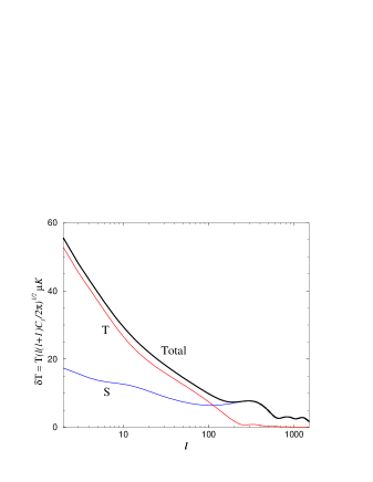
FIG. 6.: The spectrum of temperature anisotropies predicted for the exponential Hawking-Turok model described in appendix D. We have choosen the cosmological parameters $h=0.70$, $\Omega_{m}=0.35$, $\Omega_{B}$=0.05, $\Omega_{\Lambda}=0$, $Y_{He}=0.24$, and $N_{\nu}=3.04$. We show the individual contributions from the scalar (S) and tensor (T) modes, as well as the total contribution. Since inflation never ends for an exponential potential, we have artificially truncated the potential so that the number of e-foldings corresponds to a present value of the density parameter $\Omega_{0}=0.4$. Notice that the spectrum is finite in spite of the singular nature of the background.

2 Tensor power spectrum

For the present model, the equation (54) for the tensor perturbation variable ${\mathchoice{{\hbox{\boldmath$\displaystyle w$}}}{{\hbox{\boldmath$\textstyle w$}}}{{\hbox{\boldmath$\scriptstyle w$}}}{{\hbox{\boldmath$\scriptscriptstyle w$}}}}^{p}$ coincides with the one for ${\mathchoice{{\hbox{\boldmath$\displaystyle q$}}}{{\hbox{\boldmath$\textstyle q$}}}{{\hbox{\boldmath$\scriptstyle q$}}}{{\hbox{\boldmath$\scriptscriptstyle q$}}}}^{p}$,

$$-{\mathchoice{{\hbox{\boldmath$\displaystyle w$}}}{{\hbox{\boldmath$\textstyle w$}}}{{\hbox{\boldmath$\scriptstyle w$}}}{{\hbox{\boldmath$\scriptscriptstyle w$}}}}^{\prime\prime}_{p}+\frac{3}{\sinh^{2}2\eta_{C}}{\mathchoice{{\hbox{\boldmath$\displaystyle w$}}}{{\hbox{\boldmath$\textstyle w$}}}{{\hbox{\boldmath$\scriptstyle w$}}}{{\hbox{\boldmath$\scriptscriptstyle w$}}}}_{p}=p^{2}{\mathchoice{{\hbox{\boldmath$\displaystyle w$}}}{{\hbox{\boldmath$\textstyle w$}}}{{\hbox{\boldmath$\scriptstyle w$}}}{{\hbox{\boldmath$\scriptscriptstyle w$}}}}_{p}.$$ (D14)

The reflection coefficient in Eq. (151) for the tensor perturbation is then the one computed in the previos section, Eq. (D7), and the solution $\mathchoice{{\hbox{\boldmath$\displaystyle\widetilde{w}$}}}{{\hbox{\boldmath$\textstyle\widetilde{w}$}}}{{\hbox{\boldmath$\scriptstyle\widetilde{w}$}}}{{\hbox{\boldmath$\scriptscriptstyle\widetilde{w}$}}}^{p}$ coincides with $\mathchoice{{\hbox{\boldmath$\displaystyle\tilde{q}$}}}{{\hbox{\boldmath$\textstyle\tilde{q}$}}}{{\hbox{\boldmath$\scriptstyle\tilde{q}$}}}{{\hbox{\boldmath$\scriptscriptstyle\tilde{q}$}}}^{p}$, Eq. (D8).

Collecting these results, the tensor transfer function (166) for this model is given by

$${\cal T}_{T}^{p}=-\frac{2\kappa H_{0}}{\sqrt{2\pi}}\frac{\Gamma(1+ip/2)}{(p^{2}+1)\Gamma(3/2+ip/2)}\,,$$ (D15)

and the power spectrum by

$$\langle|U_{p\ell m}^{(+)}|^{2}\rangle=|\tilde{\cal N}^{T}_{p}|^{2}\left<\left|\frac{Q^{p}_{T}}{a^{2}}\right|^{2}\right>=\frac{8\kappa H_{0}^{2}}{\pi(p^{2}+1)^{2}}\,.$$ (D16)

The power spectrum of temperature anisotropies predicted for this model due to tensor perturbations is shown in Fig. 6.

REFERENCES

- [1] J. R. Gott III, Nature 295, 304 (1982); J.R. Gott and T.S. Stalter, Phys. Lett. B 136, 157 (1984); A. Guth and E. Weinberg, Nucl. Phys. B212, 321 (1983).
- [2] S. Coleman, Phys. Rev. D 15, 2929 (1977); S. Coleman and F. De Luccia, Phys. Rev. D 21, 3305 (1980).
- [3] M. Sasaki, T. Tanaka, K. Yamamoto and J. Yokoyama, Phys. Lett. B 317, 510 (1993); K. Yamamoto, M. Sasaki and T. Tanaka, Astrophy. J. 455, 412 (1995).
- [4] M. Bucher, A. Goldhaber and N. Turok, Phys. Rev. D 52, 3314 (1995); M. Bucher and N. Turok, ibid. 52, 5538 (1995); M. Bucher, A. Goldhaber and N. Turok, Nucl. Phys. B, Proc. Suppl. 43, 173 (1995).
- [5] A. Linde. Phys. Lett. B 351, 99 (95); A. Linde and A. Mezhlumian, Phys. Rev. D 52, 6789 (1995); A.M. Green and A.R. Liddle, Phys. Rev. D 55, 609 (1997).
- [6] A.D. Linde, hep-ph/9807493; A.D. Linde, M. Sasaki, T. Tanaka, astro-ph/9901135.
- [7] J. Garriga, T. Tanaka and A. Vilenkin, astro-ph/9803268 (1998).
- [8] M. Sasaki and T. Tanaka, Phys. Rev. D 54, 4705 (1996).
- [9] J. Garcia-Bellido, J. Garriga and X. Montes, Phys. Rev. D 57, 4669 (1998); J. Garcia-Bellido, J. Garriga and X. Montes, hep-ph/9812533.
- [10] S.W. Hawking and N. Turok, Phys. Lett. B425, 25 (1998).
- [11] A. Vilenkin, Phys. Rev. D 57, 7069 (1998); A. Linde, Phys. Rev. D 58, 083514 (1998); W. Unruh, gr-qc/9803050 (1998).
- [12] J. Garriga, hep-th/9803210 (1998).
- [13] J.D. Cohn, Phys. Rev. D 58, 063507 (1998).
- [14] T. Vachaspati and A. Vilenkin, Phys. Rev. D 43, 3846 (1991); T. Tanaka, M. Sasaki and K. Yamamoto, Phys. Rev. D 49, 1039 (1994); T. Tanaka and M. Sasaki, Phys. Rev. D 50, 6444 (1994); S. Mukohyama, Phys. Rev. D 56, 7638 (1997).
- [15] J.J. Halliwell and S.W. Hawking, Phys. Rev. D38, 1777 (1985).
- [16] J. Garriga, X. Montes, M. Sasaki and T. Tanaka, Nucl. Phys. B 513, 343 (1998); Erratum xxx.
- [17] T. Hamazaki, M. Sasaki, T. Tanaka, K. Yamamoto, Phys. Rev. D53, 2045 (1996); J. Garriga and V. F. Mukhanov, astro-ph/9702201; J. Garcia-Bellido, Phys. Rev. D 56, 3225 (1997); J. Garcia-Bellido and A.R. Liddle, Phys. Rev. D 55, 4603 (1997); J. Garcia-Bellido, A.R. Liddle, D.H. Lyth and D. Wands, Phys. Rev. D 55, 4596 (1997); J.D. Cohn, Phys. Rev. D 54, 7215 (1996).
- [18] K. Yamamoto, M. Sasaki and T, Tanaka, Phys. Rev. D 54, 5031 (1996).
- [19] D. Lyth and A. Woszczyna, Phys. Rev. D 52, 3338 (1995).
- [20] M. Sasaki, T. Tanaka and Y. Yakushige, Phys. Rev. D 56, 616 (1997).
- [21] T. Tanaka and M. Sasaki, Prog. Theor. Phys. 97, 243 (1997).
- [22] M. Bucher and J. Cohn, Phys. Rev. D 55 7461 (1997).
- [23] K. Tomita, Prog. Theor. Phys. 68, 310 (1982).
- [24] T. Tanaka and M. Sasaki, gr-qc/9808018, to be published in Phys. Rev. D.
- [25] M. Sasaki, T. Tanaka and K. Yamamoto, Phys. Rev. D 51, 2979 (1995).
- [26] For a review, see e.g. F. Cooper et al., Phys. Rept. 251 (1995) 267.
- [27] S. Fubini, Nuovo Cimento 34A, 521 (1976).
- [28] A.D. Linde, Nucl. Phys. B216, 421 (1983); K. Lee and E. Weinberg, Nucl. Phys. B 267, 181 (1986).
- [29] N.D. Birrell and P.C.W. Davies, ‘Quantum fields in curved space’ (Cambridge University Press, Cambridge, 1982).
- [30] T. Tanaka and M. Sasaki, Phys. Rev. D 55, 6061 (1997).
- [31] J. Garriga, hep-th/9804106 (1998).