Chaos may make black holes bright

Abstract

Black holes cannot be seen directly since they absorb light and emit none, the very quality which earned them their name. We suggest that black holes may be seen indirectly through a chaotic defocusing of light. A black hole can capture light from a luminous companion in chaotic orbits before scattering the light in random directions. To a distant observer, the black hole would appear to light up. If the companion were a bright radio pulsar, this estimate suggests the black hole echo could be detectible.

Black holes evade direct detection precisely because they are black. The existence of black holes hidden behind accretion disks or in the centers of galaxies have been inferred from astrophysical observations. Despite these indirect observations, we cannot know for certain that the compact objects lurking there are in fact Einstein’s black holes. Any detection which can see in very near to the event horizon would provide more incriminating evidence for their existence. In this Letter we describe how chaotic scattering of light in an inner regime around the event horizon could effectively render the black hole bright. If perturbed, a stochastic region develops around the last unstable photon orbit. The disturbance could be an orbiting companion or the emission of gravitational waves or any asymmetry in the evolution. The black hole can then trap incident photons in the stochastic region for some time before throwing off half and absorbing the other half, effectively shrouding it in light. We estimate the cross-section for this gravitational defocusing generically and then illustrate with an extremal binary black hole spacetime.

Around an isolated black hole of mass $M$ and charge $Q$, light follows the simple orbits

$$\left(dR\over d\phi\right)^{2}={R^{4}\over b^{2}}-R^{2}\left(1-{2M\over R}+{Q^{2}\over R^{2}}\right)\ \ .$$ (1)

The motion of massless particles depends only on the impact parameter $b=L/E$ and not on the energy $E$ and the angular momentum $L$ separately. Given the mass and charge of the black hole, there is a critical value of the impact parameter, $b_{c}$, at which light gets trapped in a perfectly circular, unstable orbit. For smaller impact parameters, light will fall into the black hole while for larger impact parameters, light escapes. Just above $b_{c}$, the light can come close to the circular orbit executing one or more full rotations before being cast off. Only black holes are compact enough to bend light by more than $\pi$. The phenomenon of back scattering by a full $\pi$ is known as the glory [1] and was thought to be the weakest way to observe black holes.

In the stochastic region around a black hole pair, the last unstable orbit becomes the site for chaotic scattering. The lone periodic orbit is replaced by a glut of periodic orbits. These proliferating orbits are packed so densely into phase space that they form a fractal set. Fractals are a way of maximizing the area while maintaining a bounded volume. Light scatters chaotically as it skips from one periodic orbit to another. The cross-section for catching light in multiple windings around the hole is then amplified. As well, the black hole hangs on to the light for longer and reemits the light more evenly. A bright light directed onto the black hole, say from a pulsar companion, could illuminate the black hole for a time before the light decayed away and the star fell dark again.

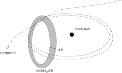
FIG. 1.: A black hole with a bright companion captures light around $R=3M$ for a few windings before the light scatters off.

The defocusing cross-section can be approximated generally in terms of the topological features of the chaotic fractal set. The importance of the general approach is that the scattering cross-section for any candidate system can be estimated in this manner. We assume isotropy which will in fact be broken by an actual perturber. The perturbation is largest at the point of closest approach and is presumably larger in the orbital plane. This whole system is also moving relative to the observer. For the purposes of estimating the magnitude of defocusing, it is reasonable to assume isotropy. In fact, isotropy could be approached for complex orbital motions since light may no longer be confined to a plane. The cross-section $\sigma$ is roughly the geometric area of the annulus

$$\sigma=2\pi b_{c}\Delta b$$ (2)

as shown in fig. 1. As light is shot at the black hole with impact parameter near $b_{c}$, it will travel on nearly periodic orbits for a time before diverging from these unstable worldlines. The cross-sectional thickness $\Delta b$ is thus given by the number of periodic orbits times the thickness around each orbit in phase space $\epsilon$. With $N(n)$ the number of fixed points lying on periodic orbits which execute $n$ windings around the black hole, $\sigma$ can be written as a sum over all winding numbers,

$$\sigma=2\pi b_{c}^{2}\sum_{n=1}^{\infty}N(n)\epsilon(n)\ \ .$$ (3)

The number of fixed points is given by the topological entropy

$$S=\lim_{n\rightarrow\infty}{1\over n}N(n)$$ (4)

so that $N(n)\sim e^{Sn}$ in the limit of long orbits. Perturbatively, the deviation is $\delta r/r\sim\lambda$ with $\lambda$ the Lyapunov exponent, a measure of the instability of the orbit. The width in phase space is then $\epsilon(n)\sim be^{-\lambda n}$ The instability can vary from orbit to orbit. As an approximation we take $\lambda$ to be the average over all the fixed points. Although the Lyapunov exponent is a notoriously coordinate dependent quantity, in this context we are measuring the instability in units of windings around the black hole and the winding number does not vary from observer to observer. Under the assumption of ergodicity, half of the photons fall into the black hole and half are cast off, so we divide the cross-section in half to find

$$\sigma=\pi b_{c}^{2}\sum_{n=1}^{\infty}\left(\exp(S-\lambda)\right)^{n}\ \ .$$ (5)

Performing the sum gives

$$\sigma=\pi b_{c}^{2}{e^{(S-\lambda)}\over 1-e^{(S-\lambda)}}\ \ .$$ (6)

We can recast $\sigma$ in terms of the fractal properties of the set of periodic orbits. The fractal dimension is defined as

$$D=\lim_{\epsilon\rightarrow 0}{\ln N(\epsilon)\over\ln(1/\epsilon)}\ \ ,$$ (7)

where $N(\epsilon)$ is the number of boxes of size $\epsilon$ needed to cover the set. We can relate $D$ to the entropy by noting that $\epsilon\propto e^{-\lambda n}$ for orbits of length $n$, from which it follows that

$$D = \lim_{n\rightarrow\infty}{\ln N(\epsilon)\over n\lambda}$$ (8)

$$= {S\over\lambda}\ \ .$$ (9)

Again, this assumes $\lambda$ is the same across the set or that a suitable average will fare well enough. There is an entire spectrum of weighted entropies and dimensions to characterized the fractal for which similar relationships to (9) have been conjectured [2, 3]. Using (9) in (6), we then estimate the cross-section to be

$$\sigma=\pi b_{c}^{2}{e^{-\lambda(1-D)}\over 1-e^{-\lambda(1-D)}}\ \ .$$ (10)

We could have deduced the cross-section directly from the fractal property. The proliferation of periodic orbits form a fractal set which fills an area in the oribital plane. The set, by definition of the fractal dimensionality, therefore has a thickness. That thickness is determined by the fractal dimension. According to the usual determination of the width of a fractal set, the number of fixed points in the direction $dr$ which can be covered by boxes of size $\epsilon$ is given by $N\sim(\epsilon/b)^{-D}$. The length of this set is then $N\epsilon=b(\epsilon/b)^{1-D}$ with $\epsilon\sim be^{-\lambda n}$. Summing and dividing by 2 we again derive the area of eqn. (10).

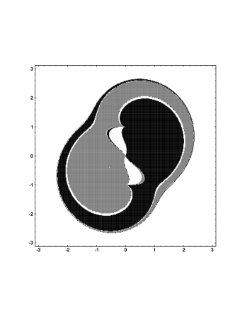
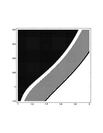
FIG. 2.: The color coded fractal basin boundaries for two extremal black holes with $Q=M=1$. The initial location of the photon is painted black if it sticks to the mass at $(0,1)$, grey if it sticks to $(0,-1)$, and white if it escapes. The initial radial velocity is $\dot{r}=0$ and $\dot{\phi}>0$ is set by eqn. (19). The error tolerance was $\sim 10^{-8}$.

We can conservatively evaluate $\sigma$ by using the unperturbed values. The dimension of the boundary is zero in the unperturbed, nonchaotic system. To estimate $\lambda$, we vary eqn. (1) around the unstable circular orbit. For a chargeless Schwarzschild black hole of mass $M$, the last unstable circular orbit lies at $R=3M$ with $b_{c}=3\sqrt{3}M$. The perturbed radial motion grows as $\delta R/R\sim e^{-\phi}$, or in units of $\phi=2\pi n$, the exponent is $\lambda=2\pi$. We then estimate $\sigma\sim{\cal O}(10^{-3})\pi b_{c}^{2}$. For an extremal black hole ($Q=M$), the last unstable circular orbit occurs at $R=2M$ with $b_{c}=4M$. At second order we find $\delta R/R\simeq e^{-\phi/\sqrt{2}}$. Measuring $\phi$ in terms of the winding number, $\phi\sim 2\pi n$, we read off $\lambda\simeq\sqrt{2}\pi$. For an extremal black hole, the cross-section is larger with $\sigma\sim{\cal O}(10^{-2})\pi b_{c}^{2}$; that is, a hundreth the capture cross-section.

Unlike other more conventional estimates of the width of a stochastic layer, this estimate requires knowledge of only a few simple properties of the system and does not require a complicated examination of the dynamical equations. Unlike other more conventional estimates, there are inherent shortcomings. As with the glory calculations [1], the effect is dominated by the trajectories which wind around the black hole the fewest number of times. These trajectories may not model the fractal set of underlying periodic orbits as well as those which execute many windings and spend the most time chaotically scattering off the set. In other words, the sum in eqn. (5) is dominated by the first few $n$ while eqn. (4) is a large $n$ limit. Given this caveat, we can see how well the approximation fares in a given dynamical system. To explicitly illustrate, we consider scattering around two extremal black holes. A pair of black holes with equal charge and mass are able to coexist in a static configuration with the electrostatic repulsion caused by their charge just balancing the gravitational attraction of their masses. While the resultant Majumdar-Papapetrou spacetime [4, 5] is static, the geodesic flows around the pair of black holes are known to be chaotic [6, 7]. We isolate fractal basin boundaries [7, 8, 9, 10, 11] for massless particles as has already been done for massive particles [7].

The Lagrangian for motion in this space can be written in isotropic coordinates as

$${\cal L}=-{1\over 2}U^{-2}\dot{t}^{2}+{1\over 2}U^{2}\left(\dot{r}^{2}+{r}^{2}\dot{\Omega}^{2}\right)$$ (11)

with $\dot{\Omega}^{2}=\sin^{2}\theta\dot{\theta}^{2}+\dot{\phi}^{2}$ and an overdot denotes differentiation with respect to an affine parameter. Schwarzschild coordinates are recovered with $R=Ur$. The metric components are determined by

$$U=1+{M\over r_{1}}+{M\over r_{2}}\ \ ,$$ (12)

where $r_{1}$ is the coordinate distance from one black hole and $r_{2}$ is the coordinate distance from the other. The event horizons occur at $r_{1}=0$ and at $r_{2}=0$. We place a black hole with mass $M$ and charge $Q=M$ at $(r,\theta,\phi)=(M,\pi/2,\pi/2)$ and an identical companion at $(M,\pi/2,-\pi/2)$ so that

$$r_{1}^{2} = r^{2}-2Mr\sin\phi+M^{2}$$ (13)

$$r_{2}^{2} = r^{2}+2Mr\sin\phi+M^{2}\ \ .$$ (14)

The geodesic motion is found by evolving the conjugate momenta, $\Pi_{q}={\partial{\cal L}/\partial\dot{q}}$. Two coordinates are automatically conserved with

$$\Pi_{t} = {\dot{t}\over U^{2}}=E$$ (15)

$$\Pi_{\theta} = r^{2}U^{2}\dot{\theta}=L_{\theta}\ \ .$$ (16)

while two are dynamical

$$\Pi_{\phi} = r^{2}U^{2}\dot{\phi}$$ (17)

$$\Pi_{r} = U^{2}\dot{r}\ \$$ (18)

and evolve according to the equations $\dot{\Pi}_{q}={\partial{\cal L}/\partial q}$. There is an additional constraint equation, equivalent to the conservation of energy obtained by setting ${\cal L}=0$ so that the photons travel along null geodesics:

$$\dot{r}^{2}+r^{2}\dot{\phi}^{2}=E^{2}\ \ .$$ (19)

We have assumed that $L_{\theta}=0$ and so consider motion in the plane defined by the binary system ($\theta=\pi/2$).

We numerically evolve the goedesic equations, ensuring that the energy is conserved according to eqn. (19). In isotropic coordinates, the last unstable circular orbit around an isolated black hole occurs at $r=M$. So, in the black hole pair, we expect to see chaos around $r_{1}=M$ and $r_{2}=M$, which is precisely what we find as illustrated by the fractal basin boundaries of fig. 2 [7, 8]. We look at an initial slice through the plane of the binary system. We submerge the black holes and their surrounding area in a bath of light, a photon at each location in space with $\dot{r}=0$ initially and $\dot{\phi}>0$ set by eqn. (19). We color code the initial location black if the photon which originated there fell into the hole at $r_{1}=0$, grey if it fell into $r_{2}=0$, and white if it escaped. The result is the mixed, fractal basin boundary as shown in fig. 2. The lower panel focuses in on one region to show the repetition of the fractal structure. The dimension of this boundary is $1+D\simeq 1.1$.

If we take $\Delta b$ to be roughly the size of the white strip in the lower panel of fig. 2, we would estimate $\delta r/M\sim 0.02$. Of course, the meaning of this coordinate thickness is ambiguous. Still it is reassuring that it is comparable in magnitude to the value we would have guessed from our generic approximation using the unperturbed $\lambda$ and the measured value of $D\sim 0.1$, which gives $\Delta b/b_{c}\sim 0.02$, although the extreme agreement is certainly fortuitous. The cross section is again about $\sigma\sim{\cal O}(10^{-2})\pi b_{c}^{2}$.

It is not immediately obvious if the approximation underestimates or overestimates the corss-section. Some elements are underestimated. For instance, there are additional contributions to the defocused light from the inner regions of the binary system which are not included in the estimate of eqn. (10). Also, any realistic astrophysical black hole with a companion will only be more chaotic than this crisp example. The metric will not be static and it is likely that the evolution of the spacetime itself will be chaotic. The companion needed to provide the luminous source may well be on an unpredictable trajectory contributing to the probability of defocusing. On the other hand, the calculation was restricted to the orbital plane where the effect would be largest and the relative orientation of the observer may decrease the signal.

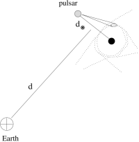
FIG. 3.: A black hole, pulsar, Earth configuration.

We can use the estimate of the cross-section from the Majumdar-Papapetrou spacetime to give rough predictions for the observability of the effect. To a distant observer, a black hole with a pulsar companion will appear to radiate with a luminosity

$$L_{\rm BH}\simeq L_{*}\left(\sigma\over\sigma_{beam}\right)\left(\tau_{*}\over\tau\right)\ \$$ (20)

where $L_{*}$ is the observed luminosity of the star, the binary lies at a distance $d$ from the Earth, and $d_{*}$ is the relative star and black hole separation as shown in Fig. 3. The cross-section of the beam is roughly $\pi d_{*}^{2}\sin^{2}(\theta_{beam})$ where $\theta_{beam}$ is the half-angle subtended by the pulse. We further assume that the time it takes the beam to sweep over the black hole $\tau_{*}$ is comparable to the characteristic time $\tau$ for the captured light to decay off the black hole. We take the companion to be at a distance of $d_{*}\sim 10^{n}M_{\rm BH}$. Using $\sigma\sim{\cal O}(10^{-3})\pi 27M^{2}$ and assuming $\theta_{beam}\sim 5^{o}$ we estimate

$$L_{BH}>3.6\times 10^{-2n+1}\ L_{*}\ \ .$$ (21)

Notice that this is the most pessimistic estimate. The black hole luminosity is suppressed relative to the incident luminosity by $\sigma/\sigma_{beam}$. Since $\sigma_{beam}$ is much larger than the scattering cross-section, the returned radiation looks small. However, the incident radiation can accumulate as the pulse returns again and again feuling a larger returned radiation. In fact, this is how pulsars are observed here on Earth. The entire beam luminosity is collected as the signal sweeps across the telescope. Pursuing this rough most conservative estimate for a pulsar at a distance $d_{*}=100M$, a signal $10^{-4}$ times fainter would be seen just behind the original pulse. The luminosity is also transient, decaying in a timescale related to the instability of the orbits. (For a solar mass black hole $\tau\sim 2GM_{\odot}/c^{3}\sim 10^{-5}-10^{-6}$ sec.) Even if the beam pointed away from the Earth, as it swept over the black hole it would feed the stochastic layer and we would see a faint echo of the unseen pulsar from the diffuse light defocused off the black hole. The gravitational Doppler shift will also separate the frequency of the echo from that of the original pulse for nonstatic systems. As a last point, superradiance of scattered light from the ergosphere of a rotating black hole could also be significant.

A more realistic calculation will be challenging as is reflected by the imfamous full relativistic binary problem. What is clear is that as the companion gets closer, chaos will be more important and the signal will get brighter, but the lifetime of the binary will also be shorter. The last stages of inspiral may be characterized by the defocused echo in coordination with the gravity wave signal expected.

Most black hole systems currently accessible to observation involve the accretion of material from a luminous companion and the defousing effect would be completely obscured. Only in the most minimal binary pairs will the chaotic scattering lead to a visible glow around the black hole such as black hole/neutron star pairs and black hole/puslar pairs in particular. Since these are amoung the systems the future gravity wave experiments hope to discover, this could offer a valuable electromagnetic observational counterpart to any gravity wave detection. The gravity wave experiments hope to detect quite distant coalescing binaries. It is unlikely that a pulsar would ever be visible at such large distances. Nonetheless, during the last stages of inspiral tidal stresses will undoubtedly heat up the companion providing a brighter electromagnetic signal to observe. The details of such a scenario are far from clear but the possibilities are worth investigating.

While we have been promoting chaotic defocusing as a means to view the inner orbits around a black hole, there are other observable consequences of the chaotic flows. For instance gravity-waves are a natural and inevitable source for the perturbations [12, 13] and the implications for the direct detection of gravity-waves from the last stages of inspiral in a compact binary will certainly be significant. More immediately observable, the disrupted motions of an accretion disk around black hole candidates could lead to an indirect detection of gravity-waves. Whether in radio waves or gravity waves, chaos may in fact make black holes bright.

I am particularly grateful to Neil Cornish for numerous critical discussions. Many of these ideas grew out of our related collaborations. I also thank John Barrow, Pedro Ferreira, John Hibbard, Andrew Jaffe and Mike Eracleous for their interest and valuable comments.

REFERENCES

- [1] C.W. Misner, K.S. Thorne and J.A. Wheeler, Gravitation (W.H. Freeman and Company, New York, 1970).
- [2] C. Grebogi, E. Ott & J. A. Yorke, Phys. Rev. Lett. 50, 935 (1983).
- [3] E. Ott, Chaos in dynamical systems, (Cambridge University Press, Cambridge, 1993).
- [4] S.D.Majumdar, Phys. Rev. 72 (1947) 390.
- [5] A. Papapetrou, Proc. R. Irish Acad. A51 (1947) 191.
- [6] G. Contopolous, Proc. R. Soc. A431 (1990) 183; G. Contopolous, Proc. R. Soc. A435 (1990) 551.
- [7] C. P. Dettmann, N. E. Frankel and N. J. Cornish, Phys. Rev. D50, R618 (1994); Fractals, 3, 161 (1995).
- [8] N.J. Cornish and J.J. Levin, Phys. Rev. D 53 (1996) 3022.
- [9] N.J. Cornish and J.J. Levin, Phys. Rev. Lett. 78 (1997) 998; N.J. Cornish and J.J. Levin, Phys. Rev. D.55 (1997) 7489.
- [10] N.J.Cornish and G.W.Gibbons, Class. Quantum Grav. 14 (1997) 1865.
- [11] J.D.Barrow and J.Levin, Phys. Rev. Lett., 80 (1998) 656.
- [12] L. Bombelli and E. Calzetta, Class. Quantum. Grav. 9 (1992) 2573.
- [13] R. Moeckel, Commun. Math. Phys. 150 415 (1992).