Effect of the Magellanic Clouds on the Milky Way disk
and VICE VERSA

Abstract

The satellite-disk interaction provides limits on halo properties in two ways: (1) physical arguments motivate the excitation of observable Galactic disk structure in the presence of a massive halo, although precise limits on halo parameters are scenario-dependent; (2) conversely, the Milky Way as a whole has significant dynamical effect on LMC structure and this interaction also leads to halo limits. Together, these scenarios give strong corroboration of our current gravitational mass estimates and suggests a rapidly evolving LMC.

Department of Physics & Astronomy, University of Massachusetts, Amherst, MA 01003-4525, USA

1 Introduction

Previous attempts at disturbing the Galactic disk by the Magellanic Clouds relied on direct tidal forcing. However, by allowing the halo to actively respond rather than remain a rigid contributor to the rotation curve, the Clouds may produce a wake in the halo which then distorts the disk. I will describe this dynamical interaction and present results based on both linear theory and n-body simulations (§2).

Even without a massive satellite, these same physical processes may be responsible for exciting disk structure. For example, persistent halo structure may result from discrete blobs, dark clusters and poorly mixed streams of material within the halo or from past fly-bys or minor merger events.

Finally, the tables turned, the Milky Way halo has a profound effect on LMC structure (§3). Dynamical arguments lead to a consistent determination of LMC and Milky Way Halo mass and a prediction of the LMC stellar halo by tidal heating. A fractionally more massive spheroid has implications for microlensing optical depth.

2 Scenario #1: LMC disturbs Halo $\rightarrow$ Halo disturbs Disk

2.1 Mechanism overview

The basic physics is well-understood: a perturbation external to a galaxy excites a wake in the halo. For a satellite, this perturbation is outside the disk but peaks in the halo near the satellite location. The gravitational force of wake then attracts the satellite; this is dynamical friction. An n-body example of this wake is shown in Figure 1.

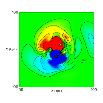
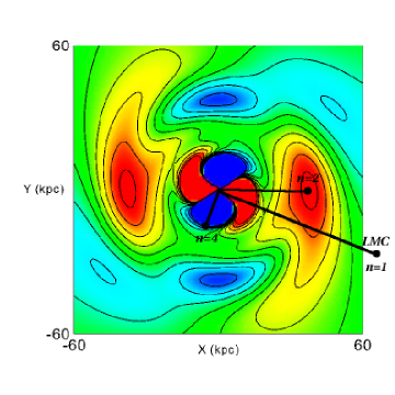
Figure 1: Wake from n-body simulation for Milky Way and LMC interaction. Left: density wake due to LMC-like satellite viewed in orbital plane. The negative (positive) overdensity is color deep red (deep blue). The peak relative density is $\approx 15\%$. Current orbital radius is nearly that of a circular orbit with the same energy. Right: Blow up showing quadrupole component only. The peak relative density is a factor of two smaller than in the left-hand panel. The radial location of the $n=1,2,4$ resonances are shown. These features agree nicely with the analytic predictions (Weinberg 1998).

Although the peak in relative density is near the perturber, the quasi-periodic satellite orbit resonates with orbits at higher-frequency and smaller radii. This permits harmonics of the primary response to produce a non-local wake in the inner halo. For example, let us consider the LMC orbit. The characteristic orbital frequency is $\Omega_{p}\equiv V_{o}/r_{mean}$; in other words, choose $r_{mean}$ to yield the correct azimuthal orbital frequency for the flat rotation curve with value $V_{o}$. The $n:1$ resonances are defined by $m\Omega-\Omega(r)=0$ or at characteristic radii given by $r\sim r_{mean}/n$. For $r_{mean}\approx 70{\rm\,kpc}$ (cf. LMC orbit), the $n=2,4$ harmonics are at 35 and 17.5 kpc, respectively (see Fig. 1). The lowest radial and angular orders have the largest amplitudes. In particular, the $m\mathrel{\hbox to0.0pt{\lower 3.0pt\hbox{$\mathchar 536\relax$}\hss}\raise 2.0pt\hbox{$\mathchar 316\relax$}}2$ angular harmonics have the range and amplitude to measurably distort the disk as will be described below.

2.2 Some subtleties: modes and resonances

As in any dynamical system, the evolution of a galaxian halo to a perturbation depends on its underlying modal structure. In stellar systems, there are both discrete and continuous modes. The continuous modes are excited as a sort of wave packet which disperses though phase mixing. In some cases, the discrete modes will dominate the response. For a dynamically stable halo, these are damped modes. Because all responses are superpositions of the same modes, the response will be similar in overall appearance for widely varying perturbations.

The pattern speeds of these lowest-order modes tend to be very small. There is a good reason for this: this frequency must be in a range relatively devoid of commensurabilities with the internal stellar orbits. As a consequence they respond most strongly to low-frequency external forcing. Relative to characteristic inner galaxy orbital frequencies, the frequencies of a distant orbiting satellite are quite small indeed, and therefore can easily drive the low-order natural modes. In this case, we expect the modes to be entrained by and follow the position angle of the disturbance.

2.3 Consequences

In the case of the LMC–Galaxy interaction, the halo wake and disk modes conspire to produce structure as follows:

Figure 2: Warp in Milky Way disk due to LMC. Each unit in $X$ and $Y$ is 7 kpc. Each unit in height is 2.1 kpc. From Weinberg (1998).

1. The $l=2$ halo distortion due to a satellite on a polar orbit—such as the LMC—can excite an $m=1$ vertical disturbance in the disk: a warp. The relative density in the satellite-induced halo distortion near the outer disk is roughly $5\%$. Although this is only enough for a low-amplitude warp, the disk response, is also a superposition of modes and the disk warping is dominated by the excitation of discrete bending modes. If the wake pattern frequency is approximately commensurate with the disk bending frequency, a significant amplification can result in kiloparsec-scale warps.

   As an aside, for n-body simulations with fewer than several hundred thousand halo particles, the Poisson noise is sufficient to raise the low-order modes to the same amplitude. The difference here is that the phase is stochastically varying in time whereas the periodic forcing yields the resonant amplification.

   Figure 2 shows an example for Milky Way–LMC parameters. The warp follows the halo distortion and therefore has a retrograde pattern speed.

   

   Figure 3: Predicted dipole distortion in Milky Way caused by LMC halo wake. Left: $m=1$ in-plane distortion Right: isodensity profiles for large LMC mass ($M=2\times 10^{10}{\rm\,M_{\odot}}$, see §3).

2. The $l=1$ in-plane distortion can be quite large although it produces no warp. Both theory and N-body simulations predict dish-like vertical distortions resulting from $l=1$ disturbances. Also significant, the $m=1$ distortion in the Galactic plane is at the 10–20% level although the corresponding change in radial velocity is rather small (Fig. 3).

A vertical warping presents a vertical velocity distortion as a diagnostic. Earlier this year Smart et al. (Smart et al. 1998) inferred the nearby vertical velocity distortion using proper motions of O-B stars. The prediction from the model has a similar trend to the Smart et al. inference but lower amplitude.

2.4 Some n-body surprises

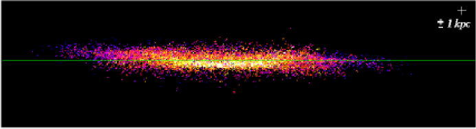
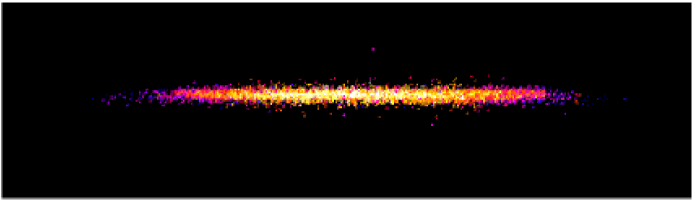
Figure 4: N-body simulation of LMC-Milky Way interaction (N=500,000). The satellite is approaching pericenter below the plane. Upper: edge on view of warped disk. The inset cross shows $\pm 1{\rm\,kpc}$. Lower: edge of view of the using same initial conditions but without satellite.

Figure 4 shows the results of n-body simulation of a disk-halo with and without a satellite perturber. A recent paper by Velasquez & White (1998) describes a warp excitation using rings. Although I have not made a detailed comparison, their warp appears consistent with these predictions.

My previous analysis has concentrated on the $l=2$ distortion because of its role in producing the “integral sign” warp. However, as Figure 1 clearly shows, the $l=1,m=1$ component is significant. The first panel in the figure shows the $l\geq 1$ harmonics is dominated by the inner $m=1$ component. In fact, this is due to the existence of a weakly damped $m=1$ halo mode (Weinberg 1994). Since the LMC orbit is roughly polar, the inner galaxy is periodically accelerated northward and southward on a roughly gigayear time scale. This leads to both a corrugated bending and disk heating (see also Edelsohn & Elmegreen 1997). The disk heating in Figure 4 may be exacerbated by particle noise.

2.5 Summary: limits on the halo mass and profile

1. The halo wake is not the only possible mechanism for producing warps (Binney 1992, Binney et al. 1997, Jiang & Binney 1998). Nonetheless, it appears the LMC can have observable effects on the Milky Way disk. The magnitude of these effects depends in part on the mass of the LMC and we will explore this in detail below.

2. For a Milky Way halo mass of $5\times 10^{11}{\rm\,M_{\odot}}$ inside of 50 kpc, the LMC can both produce the magnitude of the observed warp and arrange observable $m=1$ distortions (e.g. the inner-disk offset and a predicted outer disk offset).

3. A less massive halo than the 10:1 ratio is inconsistent with the rotation curve and leads to disk instability. Nonetheless, similar warp amplitudes persist until about 7.5:1 beyond which the effect of the wake on the disk decreases.

   However, the halo-disk interaction is diminished if the halo mass is increased by 50%–100%. As the halo mass increases, the orbital frequency increases. This detunes the disk bending mode and decreases the excitation of the inner $m=1$ mode.

3 Scenario #2: Halo disturbs LMC

A reliable estimate of the disk effects due to LMC disturbance requires a reliable estimate of the LMC mass and orbit. Recent proper motion measurements (Jones et al. 1994) combined with simulations has helped secure the orbital parameters. The standard mass estimates, however, vary by a factor or three! In addition, the time-dependent tidal forcing of the LMC along its orbit has dramatic consequences for the internal dynamics of the LMC. I will describe initial investigations into both below. These avenue of inquiry leads to firm estimates.

3.1 Mass & Structure of LMC

There have been a wide variety of LMC studies, most of which treat the LMC as a separate galaxy and use the standard mass and mass density estimates: rotation curves, star counts, surface brightness profiles.

Two relatively recent and often-cited rotation curve studies, Meatheringham et al. (1988) and Schommer et al. (1992), estimate LMC masses of $6\times 10^{9}{\rm\,M_{\odot}}$ and $1.5\times 10^{10}{\rm\,M_{\odot}}$. The main difference between these two is not the values of $V_{c}$ but the radial extent of the curve.

Alternatively, from the Milky Way’s point of view, the LMC is an oversize globular cluster. Its tidal radius is measurable and depends on both the Milky Way rotation curve and the LMC mass (and, weakly, its profile). This gives us additional checks and limits on both the Milky Way halo profile and the LMC mass.

3.1.1 The LMC tidal radius and mass

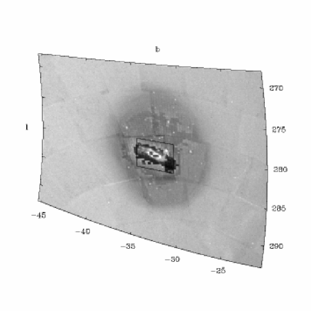
Figure 5: Stars from the LMC field from USNO-A1.0 catalog, binned on $512\times 512$ Cartesian grid centered on the LMC. Grey scale is logarithmic from zero (white) to 632 (black).

Figure  5 shows the binned star counts from the digitized POSS in the USNO-A catalog (Monet 1996). The extended stellar population extends outward to at least $10^{\circ}$ from the center (see also Irwin 1991). This population has M-giant colors. Its extent motivates a tentative identification with a halo or spheroid rather than the standard LMC disk. I will discuss a plausible dynamical explanation for this population at the end. From the extent of the stellar halo of the LMC, we can estimate the tidal radius and the mass of the Cloud. This was attempted by Nikolaev & Weinberg (1998) based on the USNO-A1.0 data. However, large extinction in B-band and poor quality of photometry ($\sim 0.5^{m}$) made it difficult to obtain the structural parameters of the LMC accurately.

The 2MASS survey, which operates in near-infrared where the interstellar extinction is much smaller and which has much better photometric accuracy allows more accurate determination of the structural parameters. During the period from 03.19.98 to 04.02.98, the 2MASS southern facility observed five $6^{\circ}\times 1^{\circ}$ fields of the Large Magellanic Cloud. The fields were selected to cover both central regions and the periphery ($\sim 5^{\circ}$) of the LMC. The positional accuracy of the scans is $\sim 1$ arc second and the photometric error is $\sim 0.03^{m}$. For this structural analysis we use only $K_{s}$-band data; additional colors can boost the sensitivity to radial density profile. We select 12 subfields $0.5^{\circ}\times 0.5^{\circ}$ in size which probe the LMC halo at the projected radii of $2^{\circ}-5^{\circ}$ from the LMC center ($l_{II}=280.5^{\circ},b_{II}=-32.9^{\circ}$). The general approach may be extended to very large datasets by hierarchical partitioning. Both this and the multicolor analysis is in progress.

We use Gaussian and power-law spherical models to describe spatial density of the LMC: $\rho\propto e^{-{r^{2}/2a^{2}}}$ and $\rho\propto\left(1+r^{2}/a^{2}\right)^{-\gamma}$. The power-law form was used by Elson, Fall & Freeman (1987) to fit the profiles of the globular clusters in the LMC, who derived $\gamma\approx 1.3$ for their sample of 10 rich clusters. We tried both fixed exponent model ($\gamma=2.0$) and models where $\gamma$ is a free parameter. We have also attempted triaxial models but invariably found that there is a degeneracy between the scale length along the line-of-sight and the luminosity function. Our multicolor analysis should also break this degeneracy.

To estimate the mass of the LMC, we fit the profiles to King models to estimate the tidal radius. Standard arguments then suggest

$$M_{LMC}=\left(r_{t}\over R_{LMC}\right)^{3}2M_{MW},$$ (1)

where $R_{LMC}$ is the distance to the LMC and $M_{MW}=5\times 10^{11}\;M_{\odot}$ is the mass of the Milky Way. The mass of the LMC which follows from this expression includes both the halo and the disk mass. This procedure will underestimate the mass for two reasons. First, simulations suggest that the observed $r_{t}$ is 75%–80% of the critical point. Second, a tidally-limited object is likely to be elongated toward the Galactic center and therefore roughly along the line of sight. For a centrally-concentrated object, the axis ratio is $a/c=1.5$. Conservatively, the first correction yields a factor of $(10/8)^{3}\approx 2$. The second increases the enclosed volume by roughly $3/2$ but whether or not this should be included depends on orientation. A reasonable correction factor is then between 2 and 3 and we conservatively choose the former.

The parameters of the best-fit models and the corresponding lower limits on the LMC mass are presented in Table 1. The bracketed term in the final column is the inferred mass with no tidal radius or orientation correction.

Table 1: Structural Parameters of the LMC Halo

Model	Scale Length	$r_{t}$ (kpc)	$M_{LMC}$
Gaussian @ 50 kpc	$2.64\pm 0.04\;kpc$	$10.8$	$2.0[1.0]\times 10^{10}M_{\odot}$
Power-Law ($\gamma=2.0$)	$2.85\pm 0.08\;kpc$	$10.8$	$2.0[1.0]\times 10^{10}M_{\odot}$

Both the profiles and the tidal radii are in excellent agreement with each other and suggest that the mass of the LMC is about $2.0\times 10^{10}M_{\odot}$. If the disk mass inside $3^{\circ}$ is about $4\times 10^{9}\;M_{\odot}$ (Meatheringham et al. 1988, De Rújula et al. 1995), then the LMC halo mass must be greater than $1\times 10^{10}\;M_{\odot}$.

As an independent check, we make a crude estimate of the mass of the LMC from the analysis of the halo population using the star counts in our fields. Most of the sources observed by 2MASS are M-giants with the absolute magnitude in $K$-band $K<-4^{m}$ (for the distance to the LMC of $50\,{\rm\,kpc}$ and 2MASS $K_{s}$-band flux limit of $14.3^{m}$). Assuming that these M giants are representative of an intermediate age population with a spheroidal distribution, we may estimate the total stellar mass using an infrared luminosity function. For this purpose, we adopt a the Galactic luminosity function in Wainscoat et al. (1992). Integrating over the luminosity function with a standard luminosity-mass relation results in stellar mass of $\approx 4\times 10^{9}\;M_{\odot}$, which is consistent.

3.1.2 Rotation curves: another consistency check

Schommer et al. (1992) summarizes the derived rotation curve for clusters, planetary nebulae and HI including the Meatheringham et al. results (see Fig. 8 from Schommer et al.). Using a luminosity function derived for an exponential disk and typical velocity dispersion in halo with a flat rotation curve, one finds that the circular velocity $V_{c}$ is roughly 20–30% larger than the rotation value $V_{o}$. For a rotation curve with $V_{o}\approx 75$ km/s, one finds a mass within 10.8 kpc of $M\mathrel{\hbox to0.0pt{\lower 3.0pt\hbox{$\mathchar 536\relax$}\hss}\raise 2.0pt\hbox{$\mathchar 318\relax$}}1.4\times 10^{10}{\rm\,M_{\odot}}$ which is nicely consistent with the tidal radius estimate. See Schommer et al. for more extensive discussion.

This consistency between the apparent tidal radius of the LMC and the dynamical mass estimate of Milky Way (which is dominated by the dark halo at $R_{LMC}$) is comforting for the dynamicist who uses Newton’s Law of Gravity on scales at least $10^{8}$ times larger than the direct solar system tests.

3.2 Milky Way heating of the LMC

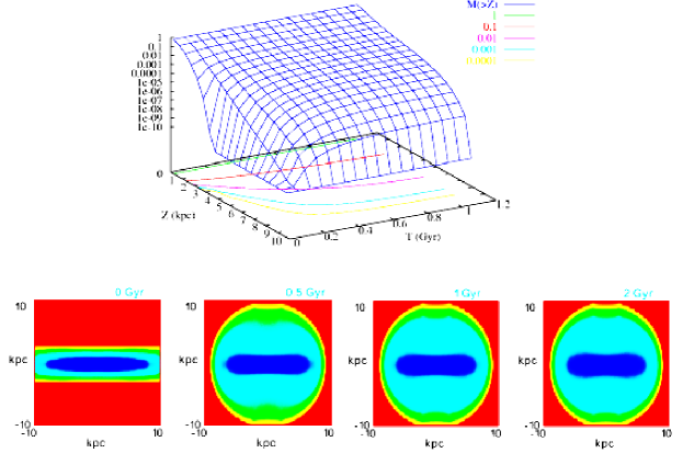
Figure 6: LMC disk heating by the Milky Way. The top panel shows the cumulative distribution of material at a height $Z$ or larger above the disk plane. The lower four panels show the projected surface density distribution for the edge on view of disk.

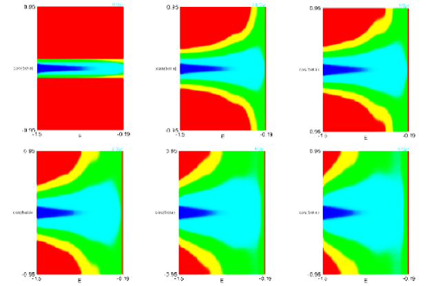
Figure 7: As in Fig. 6 but showing the phase space density in the $E$ and $\cos(\beta)\equiv J_{z}/J$ plane. Orbits with higher binding energy are ‘heated’ out of the disk plane with time.

The same dynamical couple that raises wakes in the halo affects the LMC disk. This changes the angular momentum of orbits at commensurate frequencies and “heats” the disk. To estimate the evolution, I present a solution of the time-dependent collisionless Boltzmann equation for orbits in a fixed potential. This now linear PDE is solved in a three-dimensional grid. Figure 6 shows both the cumulative mass distribution above the disk plane and projected surface mass density. Approximately 1% of the disk mass has a height larger than 6 kpc and 10% above 3 kpc after 1 Gyr. This leads to a very thick disk or flattened spheroid population. These values are underestimates since the self-consistent readjustment of the potential will lead to further heating. Although the projected profile appears unchanged for $T>1$ Gyr, this is an artifact of projection. The orbits at low binding energy are heated first and those at successively higher binding energy as time goes on. This is clearly seen in the $E$–$\cos(\beta)$ projection phase space distribution (Fig. 7). Also worthy of note is that $\log M(<Z)$ is roughly linear with $Z$ which suggests an exponential profile. A similar profile has been reported for the RR Lyrae distribution in the LMC halo (Kinman et al. 1991). The sharp roll over at the tidal radius is suggestive but may be an artifact of the particular imposition of the tidal boundary.

3.3 Microlensing

An extended LMC halo can enhance the microlensing optical depth due to self lensing. We calculate the optical depth due to microlensing assuming our spherical Gaussian halo model and the disk model from Wu (1994):

$$\rho_{D}=\rho_{0}\>e^{-R/h}\mathop{\rm sech}\nolimits^{2}(z/z_{0}),$$ (2)

where $h=1.6\;$kpc and $z_{0}=0.43\;$kpc. For now, the inclination of the LMC disk (values range from $27^{\circ}$ to $45^{\circ}$) is ignored. The mass of the LMC disk (out to $3^{\circ}$) of $4\times 10^{9}\;M_{\odot}$ (De Rújula et al. 1995) implies $\rho_{0}=0.29\;M_{\odot}/pc^{3}$. The halo mass, then, is $6\times 10^{9}\;M_{\odot}$. The optical depth averaged along the line-of-sight is computed following Kiraga & Paczyński (1994) with $\beta=-1$.

3.3.1 Results

First, assume there is no Galactic halo MACHOS: both source density $\rho_{s}$ and deflector density $\rho_{d}$ include only the stellar halo and the disk of the LMC. This gives the total optical depth due to LMC self lensing of $1.7\times 10^{-7}$; $55\%$ of this is due to halo lenses. A LMC halo mass of $1.2\times 10^{10}\;M_{\odot}$ yields the observed microlensing optical depth $2.9^{+1.4}_{-0.9}\times 10^{-7}$ (MACHO collaboration). The prediction will still be consistent with the reported value at the lower $1\sigma$ limit if the mass of the halo is $8\times 10^{9}\;M_{\odot}$. For a model consisting only of LMC halo lenses, the optical depth is $1.9\times 10^{-7}$ for halo mass $1.0\times 10^{10}\;M_{\odot}$. A halo mass of $1.1\times 10^{10}\;M_{\odot}$ yields a lensing prediction consistent at $1\sigma$ level.

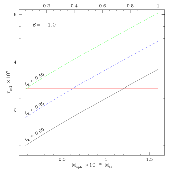
Figure 8: Predicted microlensing depth $\tau$ vs. LMC spheroid mass. The three horizontal lines show the MACHO collaboration value and errorbars. The curves show the predicted depth due to LMC lensing for Galactic MACHO fractions as labeled.

If one now adds lensing by the Galactic MACHOs, the observed optical depth is obtained for a MACHO fraction $f_{MACHO}=0.25$ (assuming the LMC mass of $1.0\times 10^{10}\;M_{\odot}$). This is marginally consistent with the estimate $f_{MACHO}=0.5^{+0.3}_{-0.2}$ obtained by the MACHO collaboration. These results are summarized in Figure 8

The inclination of the disk can enhance the optical depth and therefore can allow less massive halo to produce the observed optical depth. This is similar to Gould’s (1993) suggestion that the optical depth can show asymmetric component for different lines-of-sight through the LMC ($\sim 20\%$ asymmetry).

4 Summary

I hope to have convinced you that the natural dynamics of galaxian halos provides a mechanism for carrying disturbances from the extragalactic environment to the observable luminous disk.

In particular, the orbiting LMC should have a profound effect on the Milky Way. For halo to disk ratios of ten to one and an estimate of the LMC orbit based on its inferred space velocity, the halo wake can excite a bending mode resulting in an observed disk warp. A very heavy or centrally concentrated halo can suppress the predicted warp amplitude by detuning the near commensurability between the wake pattern speed and bending mode. In addition and independent of the warp, the halo wake causes an in-plane $m=1$ distortion of roughly 20% in the outer stellar disk. This amplitude is similar to that inferred from HI (Henderson et al. 1982). I have most thoroughly explored the LMC–Milky Way example presented here but fly-bys in group and cluster environments cause similar excitation.

The importance of the LMC to Milky Way structure has led me to consider the consequences to the LMC in more detail. From the LMC-centric viewpoint, the Milky Way is in orbit about the Cloud. Because of the mass ratio, the Milky Way forcing is a huge effect on the LMC! The simplest effect is tidal limitation and leads to a mass estimate $M_{LMC}\approx 2\times 10^{10}{\rm\,M_{\odot}}$. In fact, there is dynamical consistency between Milky Way halo rotation curve, LMC rotation curve and LMC tidal radius which corroborates our large mass estimate. Furthermore, I have argued that the time-dependent forcing perturbs the LMC well-inside of the tidal radius, exploiting the same non-local resonant mechanisms that cause the Milky Way halo wake. Because the LMC disk is inclined to its orbital radius, LMC disk orbits may be torqued by Milky Way tide producing an extended and rotating spheroid component. This prediction is consistent with the observation that nearly all LMC components have the disk kinematics (Olszewski et al. 1996). Finally, if the existence extended stellar component is borne out, LMC–LMC gravitational microlensing rates will be enhanced. Conversely, if the LMC stellar component is confirmed to be thin, we have misunderstood a basic feature of LMC dynamics.

This work was supported in part by NSF AST-9529328 and NASA/JPL 961055.

Binney, J. 1992, ARAA, 30, 51 Binney, J., and Tremaine, S. 1987, Galactic Dynamics, Princeton University Press. Binney, J., Jiang, I.-J., and Dutta, S. 199, , 297, 1237 De Rújula, A., Giudice, G. F., Mollerach, S., Roulet, E. 1995, , 275, 545 Edelsohn D. J. and Elmegreen, B. G. 1997, , 287, 947 Elson, R. A. W., Fall, S. M., Freeman, K. C. 1987, , 323, 54 Henderson, A. P. Jackson, P. D., and Kerr, F. J., , 263, 116 Irwin, M. J. 1991, in The Magellanic Clouds, ed. R. Haynes and D. Milne, Klewer, Dordrecht, 453 Jiang, I. G., and Binney, J. 1998, preprint Jones, B. F., Klemola, A. R., and Lin, D. N. C. 1994, , 107, 1333 Kinman, T. D., Stryker, L. L., Hesser, J. E., Graham, J. A., Walker, A. R., Hazen, M. L. and Nemec, J. M. 1991, , 103, 1279 Kiraga, M., Paczyński, B. 1994, ApJ, 430, L101 Meatheringham, S. J., Dopita, M. A., and Ford, H. C. 1988, , 327, 651 Monet, D. 1996, USNO-A1.0 astrometric reference catalog, U. S. Naval Observatiory. Nikolaev, S., and Weinberg, M. D. 1998, BAAS, 192, 5503 Olszewski, E. W., Suntzeff, N. B., and Mateo, M. 1996, , 34, 511 Schommer, R. A., Olszewski, E. W., Suntzeff, N. B., and Harris, H. C. 1992, , 103, 447 Smart, Drimmel, Latanzi & Binney 1998, Nature, 2 Apr 98 Tremaine, S., and Weinberg, M. D. 1984, , 209, 729 Velasquez & White 1998, preprint (astro-ph/9809412) Wainscoat, R. J., Cohen, M., Volk, K., Walker, H. J., Schwartz, D. E. 1992, , 83, 111 Weinberg, M. D. 1994, , 421, 481 Weinberg, M. D. 1998, , 299, 499 Wu, X.-P. 1994, , 435, 66