Cosmic Microwave Background Anisotropies from Scaling Seeds:
Global Defect Models

Abstract

Abstract

We investigate the global texture model of structure formation in cosmogonies with non-zero cosmological constant for different values of the Hubble parameter. We find that the absence of significant acoustic peaks and little power on large scales are robust predictions of these models. However, from a careful comparison with data we conclude that at present we cannot safely reject the model on the grounds of present CMB data. Exclusion by means of galaxy correlation data, requires assumptions on biasing and statistics. New, very stringent constraints come from peculiar velocities.

Investigating the large-$N$ limit, we argue that our main conclusions apply to all global $O(N)$ models of structure formation.

I Introduction

Recently, a lot of effort has gone into the determination of cosmological parameters from measurements of cosmic microwave background (CMB) anisotropies, especially in view of the two planned satellite experiments MAP and PLANCK[1]. However, we believe it is important to be aware of the heavy modeling which enters these results. In general, simple power law initial spectra for scalar and tensor perturbations and vanishing vector perturbations are assumed, as predicted from inflation. To reproduce observational data, the composition of the dark matter and the cosmological parameters as well as the input spectrum and the scalar to tensor ratio are varied[2].

We want to take a different approach: We modify the model for structure formation. We assume that cosmic structure was induced by scaling seeds. Using a simplified (and not very accurate) treatment for the photon propagation, we have already shown that some key observations can be reproduced within a very restricted family of scaling seed models[3]. Here we want to outline in detail a more accurate computation with a fully gauge-invariant Boltzmann code especially adapted to treat models with sources. In this paper we follow the philosophy of a general analysis of scaling seed models motivated in Ref. [4].

Seeds are an inhomogeneously distributed form of matter (like e.g. topological defects) which interacts with the cosmic fluid only gravitationally and which represents always a small fraction of the total energy of the universe. They induce geometrical perturbations, but their influence on the evolution of the background universe can be neglected. Furthermore, in first order perturbation theory, seeds evolve according to the unperturbed spacetime geometry.

Here, we mainly investigate the models of structure formation with global texture. This models (for $\Omega_{matter}=1$) show discrepancies with the observed intermediate scale CMB anisotropies and with the galaxy power spectrum on large scales[5]. Recently it has been argued that the addition of a cosmological constant leads to better agreement with data for the cosmic string model of structure formation [6]. We analyze this question for the texture model, by using ab initio simulation of cosmic texture as described in Ref. [7]. We determine the CMB anisotropies, the dark matter power spectrum and the bulk velocities for these models. We also compare our results with the large-$N$ limit of global $O(N)$ models, and we discuss briefly which type of parameter changes in the $2$-point functions of the seeds may lead to better agreement with data.

We find that the absence of significant acoustic peaks in the CMB anisotropy spectrum is a robust result for global texture as well as for the large-$N$ limit for all choices of cosmological parameters investigated. Furthermore, the dark matter power spectrum on large scales, $\lambda\stackrel{{\scriptstyle>}}{{\sim}}20h^{-1}{\rm Mpc}$, is substantially lower than the measured galaxy power spectrum.

However, comparing our CMB anisotropy spectra with present data, we cannot safely reject the model. On large angular scales, the CMB spectrum is in quite good agreement with the COBE data set, while on smaller scales we find a significant disagreement only with the Saskatoon experiment. Furthermore, for non-satellite experiments foreground contamination remains a serious problem due to the limited sky and frequency coverage.

The dark matter power spectra are clearly too low on large scales, but in view of the unresolved biasing problem, we feel reluctant to rule out the models on these grounds. A much clearer rejection may come from the bulk velocity on large scales. Our prediction is by a factor 3 to 5 lower than the POTENT result on large scales.

Since global texture and the large-$N$ limit lead to very similar results, we conclude that all global $O(N)$ models of structure formation for the cosmogonies investigated in this work are ruled out if the bulk velocity on scales of $50h^{-1}$Mpc is around 300km/s or if the CMB primordial anisotropies power spectrum really shows a structure of peaks on sub-degree angular scales.

This paper is the first of a series of analyses of models with scaling seeds. We therefore fully present the formalism used for our calculations in the next section. There, we also explain in detail the eigenvector expansion which allows to calculate the CMB anisotropies and matter power spectra in models with seeds from the two point functions of the seeds alone. This section can be skipped if the reader is mainly interested in the results. Section 3 is devoted to a brief description of the numerical simulations. In Section 4 we analyze our results and in Section 5 we draw some conclusions. Two appendices are devoted to detailed definitions of the perturbation variables and to some technical derivations.
Notation:    We always work in a spatially flat Friedmann universe. The metric is given by

$\displaystyle ds^{2}=a(t)^{2}(dt^{2}-\delta_{ij}dx^{i}dx^{j})~{},$

where $t$ denotes conformal time.

Greek indices denote spacetime coordinates $(0$ to $3)$ whereas Latin ones run from 1 to 3. Three dimensional vectors are denoted by bold face characters.

II The formalism

Anisotropies in the CMB are small and can thus be described by first order cosmological perturbation theory which we apply throughout. We neglect the non-linear evolution of density fluctuations on smaller scales. Since models with seeds are genuinely non-Gaussian, the usual numerical N-body simulations which start from Gaussian initial conditions cannot be used to describe the evolution on smaller scales.

Gauge-invariant perturbation equations for cosmological models with seeds have been derived in Refs. [8, 9]. Here we follow the notation and use the results presented in Ref. [9]. Definitions of all the gauge-invariant perturbation variables used here in terms of perturbations of the metric, the energy momentum tensor and the brightness are given in Appendix A for completeness.

We consider a background universe with density parameter $\Omega_{0}=\Omega_{m}+\Omega_{\Lambda}=1$, consisting of photons, cold dark matter (CDM), baryons and neutrinos. At very early times $z\gg z_{dec}\sim 1100$, photons and baryons form a perfectly coupled ideal fluid. As time evolves, and as the electron density drops due to recombination of primordial helium and hydrogen, Compton scattering becomes less frequent and higher moments in the photon distribution develop. This epoch has to be described by a Boltzmann equation. Long after recombination, free electrons are so sparse that the collision term can be neglected, and photons evolve according to the collisionless Boltzmann or Liouville equation. During the epoch of interest here, neutrinos are always collisionless and thus obey the Liouville equation.

In the next subsection, we parameterize in a completely general way the degrees of freedom of the seed energy momentum tensor. Subsection B is devoted to the perturbation of Einstein’s equations and the fluid equations of motion. Next we treat the Boltzmann perturbation equation. In Subsection D we explain how we determine the power spectra of CMB anisotropies, density fluctuation and peculiar velocities by means of the derived perturbation equations and the unequal time correlators of the seed energy momentum tensor, which are obtained by numerical simulations. In Subsection E we give the initial conditions and a brief description of our Boltzmann code.

A The seed energy momentum tensor

Since the energy momentum tensor of the seeds, $\Theta_{\mu\nu}$, has no homogeneous background contribution, it is gauge invariant by itself according to the Stewart-Walker Lemma[10].

$\Theta_{\mu\nu}$ can be calculated by solving the matter equations for the seeds in the Friedmann background geometry (Since $\Theta_{\mu\nu}$ has no background component it satisfies the unperturbed “conservation” equations.). We decompose $\Theta_{\mu\nu}$ into scalar, vector and tensor contributions. They decouple within linear perturbation theory and it is thus possible to write the equations for each of these contributions separately. As always (unless noted otherwise), we work in Fourier space. We parameterize the scalar $(S)$ vector $(V)$ and tensor $(T)$ contributions to $\Theta_{\mu\nu}$ in the form

$$\Theta_{00}^{(S)} = M^{2}f_{\rho}$$ (1)

$$\Theta_{j0}^{(S)} = iM^{2}k_{j}f_{v}$$ (2)

$$\Theta_{jl}^{(S)} = M^{2}\left[(f_{p}+{1\over 3}k^{2}f_{\pi})\delta_{jl}-k_{j}k_{l}f_{\pi}\right]$$ (3)

$$\Theta_{j0}^{(V)} = M^{2}w^{(v)}_{j}$$ (4)

$$\Theta_{jl}^{(V)} = iM^{2}\frac{1}{2}\left(k_{j}w^{(\pi)}_{l}+k_{l}w^{(\pi)}_{j}\right)$$ (5)

$$\Theta_{jl}^{(T)} = M^{2}\tau^{(\pi)}_{ij}~{}.$$ (6)

Here $M$ denotes a typical mass scale of the seeds. In the case of topological defects we set $M=\eta$, where $\eta$ is the symmetry breaking scale[9]. The vectors $\mbox{\boldmath$w$}^{(v)}$ and $\mbox{\boldmath$w$}^{(\pi)}$ are transverse and $\tau^{(\pi)}_{ij}$ is a transverse traceless tensor,

$\displaystyle{\bf k}\cdot\mbox{\boldmath$w$}^{(v)}={\bf k}\cdot\mbox{\boldmath$w$}^{(\pi)}=k^{i}\tau^{(\pi)}_{ij}=\tau^{(\pi)\;j}_{j}=0~{}.$

From the full energy momentum tensor $\Theta_{\mu\nu}$ which may contain scalar, vector and tensor contributions, the scalar parts $f_{v}$ and $f_{\pi}$ of a given Fourier mode are determined by

$\displaystyle ik^{j}\Theta_{0j}=-k^{2}M^{2}f_{v}~{},$

$\displaystyle-k^{i}k^{j}(\Theta_{ij}-\frac{1}{3}\delta_{ij}\delta^{kl}\Theta_{kl})=\frac{2}{3}k^{4}M^{2}f_{\pi}\;.$

On the other hand $f_{v}$ and $f_{\pi}$ are also determined in terms of $f_{\rho}$ and $f_{p}$ by energy and momentum conservation,

$$\dot{f}_{\rho}+k^{2}f_{v}+{\dot{a}\over a}(f_{\rho}+3f_{p})=0~{},$$ (7)

$$\dot{f}_{v}+2{\dot{a}\over a}f_{v}-f_{p}+{2\over 3}k^{2}f_{\pi}=0~{}.$$ (8)

Once $f_{v}$ is known it is easy to extract $M^{2}w^{(v)}_{j}=\Theta_{0j}-ik_{j}M^{2}f_{v}$. For $w^{(\pi)}_{i}$ we use

$\displaystyle ik^{j}(\Theta_{lj}-\Theta_{lj}^{(S)})=-k^{2}M^{2}w^{(\pi)}_{l}~{}.$

Again, $w^{(\pi)}_{l}$ can also be obtained in terms of $w^{(v)}_{l}$ by means of momentum conservation,

$$\dot{w}^{(v)}_{l}+2({\dot{a}\over a})w^{(v)}_{l}+{1\over 2}k^{2}w^{(\pi)}_{l}=0~{}.$$ (9)

The geometry perturbations induced by the seeds are characterized by the Bardeen potentials, $\Phi_{s}$ and $\Psi_{s}$, for scalar perturbations, the potential for the shear of the extrinsic curvature, $\mbox{\boldmath$\Sigma$}^{(s)}$, for vector perturbations and the gravitational wave amplitude, $H_{ij}^{(s)}$, for tensor perturbations. Detailed definitions of these variables and their geometrical interpretation are given in Ref. [9] (see also Appendix A). Einstein’s equations link the seed perturbations of the geometry to the energy momentum tensor of the seeds. Defining the dimensionless small parameter

$$\epsilon\equiv 4\pi GM^{2}~{},$$ (10)

we obtain

$$k^{2}\Phi_{s} = \epsilon(f_{\rho}+3{\dot{a}\over a}f_{v})$$ (11)

$$\Phi_{s}+\Psi_{s} = -2\epsilon f_{\pi}$$ (12)

$$-k^{2}\Sigma^{(s)}_{i} = 4\epsilon w^{(v)}_{i}$$ (13)

$$\ddot{H}^{(s)}_{ij}+2{\dot{a}\over a}\dot{H}^{(s)}_{ij}+k^{2}H^{(s)}_{ij} = 2\epsilon\tau^{(\pi)}_{ij}~{}.$$ (14)

Eqs. (11) to (14) would determine the geometric perturbations if the cosmic fluid were perfectly unperturbed. In a realistic situation, however, we have to add the fluid perturbations in the geometry which are defined in the next subsection. Only the total geometrical perturbations are determined via Einstein’s equations. In this sense, Eqs.  (11) to (14) should be regarded as definitions for $\Phi_{s}~{},\Psi_{s}~{},{\bf\Sigma}^{(s)}$ and $H^{(s)}_{ij}$.

A description of the numerical calculation of the energy momentum tensor of the seeds for global texture is given in Section III.

B Einstein’s equations and the fluid equations

1 scalar perturbations

Scalar perturbations of the geometry have two degrees of freedom which can be cast in terms of the gauge-invariant Bardeen potentials, $\Psi$ and $\Phi$  [11, 12]. For Newtonian forms of matter $\Psi=-\Phi$ is nothing else than the Newtonian gravitational potential. For matter with significant anisotropic stresses, $\Psi$ and $-\Phi$ differ. In geometrical terms, the former represents the lapse function of the zero-shear hyper-surfaces while the latter is a measure of their 3-curvature[9]. In the presence of seeds, the Bardeen potentials are given by

$$\Psi = \Psi_{s}+\Psi_{m}~{},$$ (15)

$$\Phi = \Phi_{s}+\Phi_{m}~{},$$ (16)

where the indices _s,m refer to contributions from a source (the seed) and the cosmic fluid respectively. The seed Bardeen potentials are given in Eqs. (11) and (12).

To describe the scalar perturbations of the energy momentum tensor of a given matter component, we use the variables $D_{g}$, a gauge-invariant variable for density fluctuations, $V$, the potential of peculiar velocity fluctuations, and $\Pi$, a potential for anisotropic stresses (which vanishes for CDM and baryons). A definition of these variables in terms of the components of the energy momentum tensor of the fluids and the metric perturbations can be found in Refs. [12] or [9] and in Appendix A.

Subscripts and superscripts _γ, _c, _b or _ν denote the radiation, CDM, baryon or neutrino fluids respectively.

Einstein’s equations yield the following relation for the matter part of the Bardeen potentials[13]

$$\Phi_{m} = {4\pi Ga^{2}\over k^{2}}\big{[}\rho_{\gamma}D_{g}^{(\gamma)}+\rho_{c}D_{g}^{(c)}+\rho_{b}D_{g}^{(b)}+$$ (20)

$$\rho_{\nu}D_{g}^{(\nu)}-\{4\rho_{\gamma}+3\rho_{c}+3\rho_{b}+4\rho_{\nu}\}\Phi$$

$$+3{\dot{a}\over a}k^{-1}\{{4\over 3}\rho_{\gamma}V_{\gamma}+\rho_{c}V_{c}$$

$$+\rho_{b}V_{b}+{4\over 3}\rho_{\nu}V_{\nu}\}\big{]}$$

$$\Psi_{m} = -\Phi_{m}-{8\pi Ga^{2}\over k^{2}}\left(p_{\gamma}\Pi_{\gamma}+p_{\nu}\Pi_{\nu}\right)~{}.$$ (21)

Note the appearance of $\Phi=\Phi_{s}+\Phi_{m}$ on the r.h.s. of Eq. (20). Using the decompositions (15,16) we can solve for $\Phi$ and $\Psi$ in terms of the fluid variables and the seeds. With the help of Friedmann’s equation, Eqs. (20) and (21) can then be written in the form

$$\Phi = {1\over{2\over 3}\left({\dot{a}\over a}\right)^{-2}k^{2}{+4x_{\gamma}+3x_{c}+3x_{b}+4x_{\nu}}}\big{[}$$ (25)

$$x_{\gamma}\sigma_{0}+x_{c}D_{g}^{(c)}+xD_{g}^{(b)}+x_{\nu}\nu_{0}+$$

$$+{\dot{a}\over a}k^{-1}\left(4x_{\gamma}V_{\gamma}+3x_{c}V_{c}+3x_{b}V_{b}\right.$$

$$\left.+4x_{\nu}V_{\nu}\right)+{2\over 3}k^{2}\left({\dot{a}\over a}\right)^{-2}\Phi_{s}\big{]}$$

$$\Psi = -\Phi-2\epsilon f_{\pi}-$$ (27)

$$\left({\dot{a}\over a}\right)^{2}k^{-2}(x_{\gamma}\Pi_{\gamma}+x_{\nu}\Pi_{\nu})~{}.$$

Here we have normalized the scale factor such that $a=1$ today. The density parameters $\Omega_{\bullet}$ always represent the values of the corresponding density parameter today (Here _∙ stands for ${}_{c}~{},~{}_{\gamma}~{},~{}_{b}$ or _ν.). To avoid any confusion, we have introduced the variables $x_{\bullet}$ for the time dependent density parameters,

$$x_{\gamma,\nu} = {\Omega_{\gamma,\nu}\over\Omega_{\gamma}+\Omega_{c}a+\Omega_{b}a+\Omega_{\nu}+\Omega_{\Lambda}a^{4}}$$ (28)

$$x_{c,b} = {\Omega_{c,b}a\over\Omega_{\gamma}+\Omega_{c}a+\Omega_{b}a+\Omega_{\nu}+\Omega_{\Lambda}a^{4}}~{}.$$ (29)

The fluid variables of photons and neutrinos are obtained by integrating the scalar brightness perturbations, which we denote by ${\cal M}_{S}(t,{\bf k},{\bf n})$ and ${\cal N}_{S}(t,{\bf k},{\bf n})$ respectively, over directions, ${\bf n}$,

$$D_{g}^{(\gamma)} = {1\over 4\pi}\int{\cal M}_{S}d\Omega=\sigma_{0}$$ (30)

$$V_{\gamma} = {3i\over 16\pi k}\int({\bf k}\cdot{\bf n}){\cal M}_{S}d\Omega$$ (31)

$$= {3\over 4}\sigma_{1}^{(S)}$$ (32)

$$\Pi_{\gamma} = {-9\over 8\pi k^{2}}\int(({\bf k}\cdot{\bf n})^{2}-{1\over 3}k^{2}){\cal M}_{S}d\Omega$$ (33)

$$= 3\sigma_{2}^{(S)}$$ (34)

$$D_{g}^{(\nu)} = {1\over 4\pi}\int{\cal N}_{S}d\Omega=\nu_{0}$$ (35)

$$V_{\nu} = {3i\over 16\pi k}\int({\bf k}\cdot{\bf n}){\cal N}_{S}d\Omega$$ (36)

$$= {3\over 4}\nu_{1}^{(S)}$$ (37)

$$\Pi_{\nu} = {-9\over 8\pi k^{2}}\int(({\bf k}\cdot{\bf n})^{2}-{1\over 3}k^{2}){\cal N}_{S}d\Omega$$ (38)

$$= 3\nu_{2}^{(S)}~{}.$$ (39)

A systematic definition of the modes $\sigma_{j}$ and $\nu_{j}$ is given in the next subsection.

The equation of motion for CDM is given by energy and momentum conservation,

$$\dot{D}_{g}^{(c)}+kV_{c} = 0~{},$$ (40)

$$\dot{V}_{c}+\left({\dot{a}\over a}\right)V_{c} = k\Psi~{}.$$ (41)

During the very tight coupling regime, $z\gg z_{dec}$, we may neglect the baryon contribution in the energy momentum conservation of the baryon-photon plasma. We then have

$$\dot{D}_{g}^{(\gamma)}+{4\over 3}kV_{\gamma} = 0~{},$$ (42)

$$\dot{V}_{\gamma}-k{1\over 4}D_{g}^{(\gamma)} = k(\Psi-\Phi)~{},$$ (43)

$$D_{g}^{(b)} = {3\over 4}D_{g}^{(\gamma)}$$ (44)

$$V_{b} = V_{\gamma}~{}.$$ (45)

The conservation equations for neutrinos are not very useful, since they involve anisotropic stresses and thus do not close. At the temperatures of interest to us, $T\ll 1$MeV, neutrinos have to be evolved by means of the Liouville equation which we discuss in the next subsection.

Once the baryon contribution to the baryon-photon fluid becomes non-negligible, and the imperfect coupling of photons and baryons has to be taken into account (for a 1% accuracy of the results, the redshift corresponding to this epoch is around $z\sim 10^{7}$), we evolve also the photons with a Boltzmann equation. The equation of motion for the baryons is then

$$\dot{D}_{g}^{(b)}+kV_{b} = 0~{},$$ (46)

$$\dot{V}_{b}+\left({\dot{a}\over a}\right)V_{b} = k\Psi-{4\sigma_{T}n_{e}\Omega_{\gamma}\over 3\Omega_{b}}[V_{\gamma}-V_{b}]~{}.$$ (47)

The last term in Eq. (47) represents the photon drag force induced by non-relativistic Compton scattering, $\sigma_{T}$ is the Thomson cross section, and $n_{e}$ denotes the number density of free electrons. At very early times, when $\sigma_{T}n_{e}\gg 1/t$, the ’Thomson drag’ just forces $V_{b}=V_{\gamma}$, which together with Eqs. (42) and (46) implies (44).

An interesting phenomenon often called ’compensation’ can be important on super horizon scales, $kt\ll 1$. If we neglect anisotropic stresses of photons and neutrinos and take into account that ${\cal O}(D_{g})={\cal O}(ktV)$ and ${\cal O}(V)={\cal O}(kt\Psi)$ for $kt\ll 1$, Eqs. (25) and (27) lead to

$${\cal O}(\Phi)={\cal O}\left((kt)^{2}\Phi_{s}-2\epsilon f_{\pi}\right)~{}.$$ (48)

Hence, if anisotropic stresses are relatively small, $\epsilon f_{\pi}\ll\Phi_{s}$, the resulting gravitational potential on super horizon scales is much smaller than the one induced by the seeds alone. One must be very careful not to over interpret this ’compensation’ which is by no means related to causality, but is due to the initial condition $D_{g}~{},V\rightarrow_{t\rightarrow 0}0$. A thorough discussion of this issue is found in Refs. [13, 14, 15]. As we shall see in the next section, for textures $\Phi_{s}$ and $\epsilon f_{\pi}$ are actually of the same order. Therefore Eq. (48) does not lead to compensation, but it indicates that CMB anisotropies on very large scales (Sachs-Wolfe effect) are dominated by the amplitude of seed anisotropic stresses.

The quantities which we want to calculate and compare with observations are the CDM density power spectrum and the peculiar velocity power spectrum today

$$P(k) = \langle|D_{g}^{(c)}(k,t_{0})|^{2}\rangle$$ (49)

and (50)

$$P_{v}(k) = \langle|V_{c}(k,t_{0})|^{2}\rangle~{}.$$ (51)

Here $\langle\cdots\rangle$ denotes an ensemble average over models. Note that even though $D_{g}$ and $V$ are gauge invariant quantities which do not agree with, e.g., the corresponding quantities in synchronous gauge, this difference is very small on subhorizon scales (of order $1/kt$) and can thus be ignored.

On subhorizon scales the seeds decay, and CDM perturbations evolve freely. We then have, like in inflationary models,

$$P_{v}(k)=H_{0}^{2}\Omega_{m}^{1.2}P(k)k^{-2}~{}.$$ (52)

2 vector perturbations

Vector perturbations of the geometry have two degrees of freedom which can be cast in a divergence free vector field. A gauge-invariant quantity describing vector perturbations of the geometry is $\Sigma$, a vector potential for the shear tensor of the $\{t=$const.$\}$ hyper-surfaces. Like for scalar perturbations, we split the contribution to $\Sigma$ into a source term coming from the seeds given in the previous subsection, and a part due to the vector perturbations in the fluid,

$$\mbox{\boldmath$\Sigma$}=\mbox{\boldmath$\Sigma$}_{s}+\mbox{\boldmath$\Sigma$}_{m}~{}.$$ (53)

The perturbation of Einstein’s equation for ${\mbox{\boldmath$\Sigma$}}_{m}$ is[9]

$$k^{2}\mbox{\boldmath$\Sigma$}_{m} = 6\left({\dot{a}\over a}\right)^{2}[{4\over 3}x_{\gamma}\mbox{\boldmath$\omega$}_{\gamma}+x_{c}\mbox{\boldmath$\omega$}_{c}+$$ (55)

$$+x_{b}\mbox{\boldmath$\omega$}_{b}+{4\over 3}x_{\nu}\mbox{\boldmath$\omega$}_{\nu}]~{}.$$

Here $\mbox{\boldmath$\omega$}_{\bullet}$ is the fluid vorticity which generates the vector type shear of the equal time hyper-surfaces (see Appendix A). By definition, vector perturbations are transverse,

$$\mbox{\boldmath$\Sigma$}\cdot{\bf k}=\mbox{\boldmath$\Sigma$}_{m}\cdot{\bf k}=\mbox{\boldmath$\Sigma$}_{s}\cdot{\bf k}=\mbox{\boldmath$\omega$}_{\bullet}\cdot{\bf k}=0~{}.$$ (56)

It is interesting to note that vector perturbations in the geometry do not induce any vector perturbations in the CDM (up to unphysical gauge modes), since no geometric terms enter the momentum conservation for CDM vorticity,

$\displaystyle\dot{\mbox{\boldmath$\omega$}}_{c}+{\dot{a}\over a}\mbox{\boldmath$\omega$}_{c}=0~{},$

hence we may simply set $\mbox{\boldmath$\omega$}_{c}=0$. This is also the case for the tightly coupled baryon radiation plasma. But as soon as higher moments in the photon distribution build up, they feel the vector perturbations in the geometry (see next section) and transfer it onto the baryons via the photon drag force,

$$\dot{\mbox{\boldmath$\omega$}}_{b}+\left({\dot{a}\over a}\right)\mbox{\boldmath$\omega$}_{b}={4\sigma_{T}n_{e}\Omega_{\gamma}\over 3\Omega_{b}}[\mbox{\boldmath$\omega$}_{\gamma}-\mbox{\boldmath$\omega$}_{b}]~{}.$$ (57)

The photon vorticity is given by an integral over the vector type photon brightness perturbation, ${\cal M}_{V}$,

$$\mbox{\boldmath$\omega$}_{\gamma}=\frac{1}{4\pi}\int{\bf n}{\cal M}_{V}d\Omega~{},$$ (58)

where the integral is over photon directions, ${\bf n}$. In terms of the development presented in the next section for ${\bf k}$ pointing in $z$-direction, we obtain

$$\mbox{\boldmath$\omega$}_{\gamma}=\left(\sigma_{1,2}^{(V)}+\sigma_{1,0}^{(V)}~{},~{}\sigma_{2,2}^{(V)}+\sigma_{2,0}^{(V)}~{},~{}0\right)~{}.$$ (59)

Equivalently, we have for neutrinos

$$\mbox{\boldmath$\omega$}_{\nu} = \frac{1}{4\pi}\int{\bf n}{\cal N}_{V}d\Omega~{},$$ (60)

$$\mbox{\boldmath$\omega$}_{\nu} = \left(\nu_{1,2}^{(V)}+\nu_{1,0}^{(V)}~{},~{}\nu_{2,2}^{(V)}+\nu_{2,0}^{(V)}~{},~{}0\right)~{}.$$ (61)

The vector equations of motion for photons and neutrinos are discussed in the next section.

3 tensor perturbations

Metric perturbations also have two tensorial degrees of freedom, gravity waves, which are represented by the two helicity states of a transverse traceless tensor (see Appendix A). As before, we split the geometry perturbation into a part induced by the seeds and a part due to the matter fluids,

$$H_{ij}=H^{(s)}_{ij}+H^{(m)}_{ij}~{}.$$ (62)

The only matter perturbations which generate gravity waves are tensor type anisotropic stresses which are present in the photon and neutrino fluids. The perturbation of Einstein’s equation yields

$$\ddot{H}^{(m)}_{ij}+2\left({\dot{a}\over a}\right)\dot{H}^{(m)}_{ij}+k^{2}H^{(m)}_{ij}=$$ (63)

$$\left({\dot{a}\over a}\right)^{2}(x_{\gamma}\Pi_{ij}^{(\gamma)}+x_{\nu}\Pi_{ij}^{(\nu)})~{}.$$ (64)

The relation between the tensor brightness perturbations ${\cal M}_{T}$, ${\cal N}_{T}$ and the tensor anisotropic stresses, $\Pi_{ij}^{(\gamma)}$ and $\Pi_{ij}^{(\nu)}$ is given by

$$\Pi^{(\gamma)}_{ij} = {3\over 4\pi}\int(n_{i}n_{j}-{1\over 3}\delta_{ij}){\cal M}_{T}d\Omega~{},$$ (65)

$$\Pi^{(\nu)}_{ij} = {3\over 4\pi}\int(n_{i}n_{j}-{1\over 3}\delta_{ij}){\cal N}_{T}d\Omega~{}.~{}$$ (66)

In terms of the development presented in the next section for ${\bf k}$ pointing in $z$-direction, we have

$$\Pi^{(\gamma)}_{11} = -\Pi^{(\gamma)}_{22}={6\over 35}\sigma_{+,4}+{4\over 7}\sigma_{+,2}+{2\over 5}\sigma_{+,0}~{},$$ (67)

$$\Pi^{(\gamma)}_{12} = \Pi^{(\gamma)}_{21}={6\over 35}\sigma_{\times,4}+{4\over 7}\sigma_{\times,2}+{2\over 5}\sigma_{\times,0}~{},$$ (68)

$$\Pi^{(\nu)}_{11} = -\Pi^{(\nu)}_{22}={6\over 35}\nu_{+,4}+{4\over 7}\nu_{+,2}+{2\over 5}\nu_{+,0}~{},$$ (69)

$$\Pi^{(\nu)}_{12} = \Pi^{(\nu)}_{21}={6\over 35}\nu_{\times,4}+{4\over 7}\nu_{\times,2}+{2\over 5}\nu_{\times,0}~{}.$$ (70)

We find that the effect of anisotropic stresses of photons and neutrinos is less than 1% in the final result, and hence we have neglected them.

C The Boltzmann equation

When particle interactions are less frequent, the fluid approximation is not sufficient, and we have to describe the given particle species by a Boltzmann equation, in order to take into account phenomena like collisional and directional dispersion. In the case of massless particles like massless neutrini or photons, the Boltzmann equation can be integrated over energy, and we obtain an equation for the brightness perturbation which depends only on momentum directions[9]. As before, we split the brightness perturbation into a scalar, vector and tensor component, and we discuss the perturbation equation of each of them separately,

$${\cal M} = {\cal M}_{S}+{\cal M}_{V}+{\cal M}_{T}$$ (71)

and (72)

$${\cal N} = {\cal N}_{S}+{\cal N}_{V}+{\cal N}_{T}.$$ (73)

The functions ${\cal M}$ and ${\cal N}$ depend on the wave vector ${\bf k}$, the photon (neutrino) direction ${\bf n}$ and conformal time $t$. Linear polarization of photons induced by Compton scattering is described by the variable ${\cal M}^{(Q)}$ (the Stokes parameter $Q$) depending on the same variables. We choose for each ${\bf k}$-mode a reference system with $z$-axis parallel to ${\bf k}$. For scalar perturbations we achieve in this way azimuthal symmetry — the left hand side of the Boltzmann equation and therefore also the brightness ${\cal M}$ depend only on $\mu=(\hat{{\bf k}}\cdot{\bf n})$ and can be developed in Legendre polynomials.

The left hand side of the Boltzmann equation for vector and tensor perturbations also determines the azimuthal dependence of ${\cal M}$ for vector and tensor perturbations, as we shall see in detail.

1 scalar perturbations

We expand the brightness ${\cal M}_{S}({\bf k},{\bf n},t)$ in the form:

$${\cal M}_{S}({\bf n},{\bf k},t)=\sum_{\ell=0}^{\infty}(-i)^{\ell}(2\ell+1)\sigma^{(S)}_{\ell}(t,{\bf k})P_{\ell}(\mu),$$ (74)

where $P_{\ell}$ denotes the Legendre polynomial of order $\ell$ and $\sigma^{(S)}_{\ell}$ is the associated multipole moment. An analogous decomposition also applies to the amplitude of polarization anisotropy, ${\cal M}_{S}^{Q}({\bf n},{\bf k},t)$, and we denote the associated multipole moment by $q^{(S)}_{\ell}$.

The Boltzmann equation for scalar perturbations in the photon brightness and polarization is [9, 16]

$$\dot{\cal M}_{S}+i\mu k{\cal M}_{S}=4i\mu k(\Phi-\Psi)+$$ (76)

$$a\sigma_{T}n_{e}[D_{g}^{(\gamma)}-{\cal M}_{S}-4i\mu V_{b}-{1\over 2}P_{2}(\mu)Q]~{},$$

$$\dot{\cal M}_{S}^{(Q)}+i\mu k{\cal M}_{S}^{(Q)}=$$ (78)

$$a\sigma_{T}n_{e}[-{\cal M}_{S}^{(Q)}+{1\over 2}\big{(}1-P_{2}(\mu\big{)})Q]~{},$$

where

$$Q=\sigma_{2}^{(S)}+q^{(S)}_{0}+q^{(S)}_{2}~{}.$$

The first term on the right hand side of Eq. (76) represents the gravitational interaction (photons without collisions move along lightlike geodesics of the perturbed geometry), while the term in square brackets is the collision integral for non-relativistic Compton scattering.

Inserting expansion (74) into Eqs. (76) and (78) using the standard recursion relations for Legendre polynomials, we obtain the following series of coupled equations:

$$\dot{\sigma}^{(S)}_{0}+{k}\sigma^{(S)}_{1}=0~{},$$ (79)

$$\dot{\sigma}^{(S)}_{1}-{k\over 3}[\sigma^{(S)}_{0}-2\sigma^{(S)}_{2}]=$$ (81)

$${4\over 3}k(\Psi-\Phi)+a\sigma_{T}n_{e}[{4\over 3}V_{b}-\sigma^{(S)}_{1}]~{},$$

$$\dot{\sigma}^{(S)}_{2}-{k\over 5}[2\sigma^{(S)}_{1}-3\sigma^{(S)}_{3}]=$$ (83)

$$-a\sigma_{T}n_{e}[\sigma^{(S)}_{2}-{1\over 10}Q]~{},$$

$$\dot{\sigma}^{(S)}_{\ell}- {k\over{2\ell+1}}\left[\ell\sigma^{(S)}_{\ell-1}-(\ell+1)\sigma^{(S)}_{\ell+1}\right] =$$ (84)

$$-a\sigma_{T}n_{e}\sigma^{(S)}_{\ell}~{}, \!\!\mbox{for }~{}~{}\ell\geq 3~{}.$$ (85)

and

$$\dot{q}^{(S)}_{\ell}-{k\over{2\ell+1}}\left[\ell q^{(S)}_{\ell-1}-{(\ell+1)}q^{(S)}_{\ell+1}\right] =$$ (86)

$$+a\sigma_{T}n_{e}[-q^{(S)}_{\ell}+{1\over 2}Q(\delta_{\ell 0}+{1\over 5}\delta_{\ell 2})].$$ (87)

For the neutrinos we obtain the same equations just without collision integral

$${\cal N}_{S}({\bf n},{\bf k},t)=\sum_{\ell=0}^{\infty}(-i)^{\ell}(2\ell+1)\nu^{(S)}_{\ell}(t,{\bf k})P_{\ell}(\mu),$$ (88)

and

$$\dot{\nu}^{(S)}_{\ell}-{k\over{2\ell+1}}\left[\ell\nu^{(S)}_{\ell-1}-{(\ell+1)}\nu^{(S)}_{\ell+1}\right] =$$ (90)

$${4\over 3}k(\Psi-\Phi)\delta_{\ell 1}.$$

We are interested in the power spectrum of CMB anisotropies which is defined by

$$\left\langle{\delta T\over T}({\bf n}){\delta T\over T}({\bf n}^{\prime})\right\rangle\left|{}_{{~{}}_{\!\!({\bf n\cdot n}^{\prime}=\cos\vartheta)}}\right.={1\over 4\pi}\sum_{\ell}(2\ell+1)C_{\ell}P_{\ell}(\cos\vartheta)~{}.$$ (91)

Here $\langle\cdots\rangle$ denotes the ensemble average over models. We assume that an ’ergodic hypothesis’ is satisfied and we can interchange spatial and ensemble averages. The problem that actual observations can average at best over one horizon volume is known under the name ’cosmic variance’. It severely restricts the accuracy with which, for example, low multipoles of CMB anisotropies observed in our horizon volume can be predicted for a given model.

Using the addition theorem of spherical harmonics, one obtains, with the Fourier transform conventions adopted here, (for details see Appendix B)

$$C_{\ell}^{(S)}={1\over{8\pi}}\int k^{2}dk\langle|\sigma^{(S)}_{\ell}(t_{0},k)|^{2}\rangle~{},$$ (92)

where the superscript ^(S) indicates that Eq. (92) gives the contribution from scalar perturbations.

2 vector perturbations

Vector perturbations are very small on angular scales corresponding to $\ell\stackrel{{\scriptstyle>}}{{\sim}}500$, where Compton scattering and thus polarization become relevant. We therefore neglect polarization in this case. The Boltzmann equation for vector perturbations then reads

$$\dot{\cal M}_{V}+i{\bf k}\cdot{\bf n}{\cal M}_{V}=-4i({\bf n}\cdot{\bf k})({\bf n}\cdot\mbox{\boldmath$\Sigma$})+$$ (94)

$$a\sigma_{T}n_{e}[4({\bf n}\cdot\mbox{\boldmath$\omega$}_{b})-{\cal M}_{V}+{1\over 2}n_{ij}M_{ij}]~{},$$

where

$$n_{ij} \equiv n_{i}n_{j}-{1\over 3}\delta_{ij}~{}~{}\mbox{ and}$$

$$M_{ij} = {3\over 8\pi}\int n_{ij}{\cal M}_{V}d\Omega~{}.$$

We use coordinates for which ${\bf k}$ is parallel to the $z$-axis. Then

$\displaystyle\mbox{\boldmath$\Sigma$}=(\Sigma_{1},\Sigma_{2},0)~{}~{},~{}~{}~{}\mbox{\boldmath$\omega$}=(\omega_{1},\omega_{2},0)$

and

$\displaystyle{\bf n}=(\sqrt{1-\mu^{2}}\cos\varphi,\sqrt{1-\mu^{2}}\sin\varphi,\mu)~{}.$

With the ansatz

$${\cal M}_{V}({\bf k},{\bf n},t) = \sqrt{1-\mu^{2}}[{\cal M}_{1}^{(V)}({\bf k},\mu,t)\cos\varphi+$$ (96)

$$+{\cal M}_{2}^{(V)}({\bf k},\mu,t)\sin\varphi]~{},$$

the equations for ${\cal M}_{1,2}$ decouple and the right hand side of Eq. (94) depends only on $\mu$. Like for scalar perturbations, we expand ${\cal M}_{1,2}$ in Legendre polynomials

$${\cal M}_{\epsilon}^{(V)}(\mu,{\bf k},t)=\sum_{\ell=0}^{\infty}(-i)^{\ell}(2\ell+1)\sigma^{(V)}_{\epsilon,\ell}(t,{\bf k})P_{\ell}(\mu),$$ (97)

where ${\epsilon}=1,2$.

Eq. (94) then leads to

$$\dot{\cal M}^{(V)}_{\epsilon}+i\mu k{\cal M}^{(V)}_{\epsilon}=-4i\mu k\Sigma_{\epsilon}+$$ (99)

$$a\sigma_{T}n_{e}[4\omega_{\epsilon}^{(b)}-{\cal M}^{(V)}_{\epsilon}-i\mu{3\over{10}}(\sigma_{{\epsilon},1}^{(V)}+\sigma_{{\epsilon},3}^{(V)})]~{}.$$

With Eq. (97), this can be expressed as the following set of coupled equations for the variables $\sigma^{(V)}_{\epsilon,\ell}$.

$$\dot{\sigma}^{(V)}_{\epsilon,0}+k\sigma^{(V)}_{\epsilon,1}=a\sigma_{T}n_{e}[4\omega_{\epsilon}^{(b)}-\sigma^{(V)}_{\epsilon,0}]~{},$$ (100)

$$\dot{\sigma}^{(V)}_{\epsilon,1}-{k\over 3}[\sigma^{(V)}_{\epsilon,0}-2\sigma^{(V)}_{\epsilon,2}]=$$ (103)

$$+{4\over 3}k\Sigma_{\epsilon}-a\sigma_{T}n_{e}[{9\over 10}\sigma^{(V)}_{\epsilon,1}-{1\over 10}\sigma^{(V)}_{\epsilon,3}]~{},$$

and

$$\dot{\sigma}^{(V)}_{\epsilon,\ell}-{k\over{2\ell+1}}\left[\ell\sigma^{(V)}_{\epsilon,\ell-1}-{(\ell+1)}\sigma^{(V)}_{\epsilon,\ell+1}\right]=$$ (105)

$$-a\sigma_{T}n_{e}\sigma^{(V)}_{\epsilon,\ell}~{}~{}\mbox{ for }\ell\geq 2.$$

For neutrino perturbations we obtain the same equations up to the collision term. We repeat them here for completeness.

$$\dot{\nu}^{(V)}_{\epsilon,\ell}-{k\over{2\ell+1}}\left[\ell\nu^{(V)}_{\epsilon,\ell-1}-{(\ell+1)}\nu^{(V)}_{\epsilon,\ell+1}\right] =$$ (106)

$$+{{4\over 3}}\Sigma_{\epsilon}k\delta_{\ell 1}.$$ (107)

As for scalar perturbations, the CMB anisotropy power spectrum is obtained by integration over $k$-space. One finds (see Appendix B),

$$C_{\ell}^{(V)}={\ell(\ell+1)\over{8\pi}}\int k^{2}dk{{\langle|\sigma^{(V)}_{1,\ell+1}(t_{0},k)+\sigma^{(V)}_{1,\ell-1}(t_{0},k)|^{2}\rangle}\over{(2\ell+1)^{2}}}~{}.$$ (108)

Here the fact that there are two equal contributions from both polarization states, $\epsilon=1,2$ (statistical isotropy) is taken care of.

3 tensor perturbations

For tensor perturbations, and a wave vector ${\bf k}$ pointing into the $3$-direction, the only non vanishing components of the perturbed metric tensor are $H_{11}=-H_{22}=H_{+}$ and $H_{12}=H_{21}=H_{\times}$. Neglecting polarization, the Boltzmann equation for tensor perturbations is[9]

$$\dot{{\cal M}}_{T}+ik\mu{\cal M}_{T}=-4n^{i}n^{j}\dot{H}_{ij}$$ (110)

$$-a\sigma_{T}n_{e}[{\cal M}_{T}-{1\over 2}n_{ij}M_{ij}]~{}.$$

With the ansatz

$${\cal M}_{T}({\bf k},{\bf n},t) = (1-\mu^{2})[{\cal M}^{(T)}_{+}({\bf k},\mu,t)\cos 2\varphi+$$ (112)

$$+{\cal M}^{(T)}_{\times}({\bf k},\mu,t)\sin 2\varphi]~{},$$

the two modes ${\cal M}^{(T)}_{+,\times}$ decouple completely and the right hand side of Eq. (110) depends only on $\mu$. We can then expand the modes in terms of Legendre polynomials

$${\cal M}^{(T)}_{\epsilon}(\mu,k,t)=\sum_{\ell=0}^{\infty}(-i)^{\ell}(2\ell+1)\sigma^{(T)}_{{\epsilon},\ell}(t,{\bf k})P_{\ell}(\mu),$$ (113)

where ${\epsilon}=+,\times$. Eq. (110) now becomes

$$\dot{\cal M}^{(T)}_{\epsilon}+i\mu k{\cal M}^{(T)}_{\epsilon}=4{\dot{H}}_{\epsilon}+$$ (115)

$$+a\sigma_{T}n_{e}[-{\cal M}^{(T)}_{\epsilon}+{1\over 10}\sigma^{(T)}_{{\epsilon},0}+{1\over 7}\sigma^{(T)}_{{\epsilon},2}+{3\over 70}\sigma^{(T)}_{{\epsilon},4}]~{},$$

leading to the series of coupled equations for the coefficients $\sigma^{(T)}_{\epsilon,\ell}$

$$\dot{\sigma}^{(T)}_{\epsilon,0}+k\sigma^{(T)}_{\epsilon,1}=4{\dot{H}}_{\epsilon}+$$ (117)

$$+a\sigma_{T}n_{e}[-{9\over 10}\sigma^{(T)}_{\epsilon,0}+{1\over 7}\sigma^{(T)}_{\epsilon,2}+{3\over 70}\sigma^{(T)}_{\epsilon,4}]~{},$$

$$\dot{\sigma}^{(T)}_{\epsilon,\ell}-{k\over 2\ell+1}\left[\ell\sigma^{(T)}_{\epsilon,\ell-1}-(\ell+1)\sigma^{(T)}_{\epsilon,\ell+1}\right]=$$ (119)

$$-a\sigma_{T}n_{e}\sigma^{(T)}_{\epsilon,\ell},~{}\mbox{ for }\ell\geq 1~{}.$$

As before, the CMB anisotropy power spectrum is obtained by integration over $k$-space (see Appendix B),

$$C_{\ell}^{(T)}={1\over{8\pi}}{{(\ell+2)!}\over{(\ell-2)!}}\int k^{2}dk{{\langle|\Sigma^{(T)}_{\ell}|^{2}\rangle}\over{(2\ell+1)^{2}}}~{},$$ (120)

where

$$\Sigma^{(T)}_{\ell}={{\sigma^{(T)}_{{\epsilon},\ell-2}}\over{2\ell-1}}-{{2{(2\ell+1)\sigma^{(T)}_{{\epsilon},\ell}}}\over{(2\ell-1)(2\ell+3)}}+{{\sigma^{(T)}_{{\epsilon},\ell+2}}\over{{2\ell+3}}}~{}.$$ (121)

D Eigenvector expansion of the source correlators

In the previous subsections we have derived a closed system of linear differential equations with source terms. The source terms are linear combinations of the seed energy momentum tensor which is determined by numerical simulations. A given realization of our model has random initial conditions; the seed energy momentum tensor is a random variable. In principle we could calculate the induced random variables $D_{g}^{(c)}({\bf k},t_{0})$, $V_{c}({\bf k},t_{0})$, $\sigma^{(\bullet)}_{\ell}({\bf k},t_{0})$ etc for 100 to 1000 realizations of our model and determine the expectation values $P(k)$, $P_{v}(k)$ and $C_{\ell}$ by averaging. This procedure has been adapted in Ref. [17] for a seed energy momentum tensor modeled by a few random parameters.

In the case of a seed energy momentum tensor coming entirely from numerical simulations, this procedure is not feasible. The first and most important bottleneck is the dynamical range of the simulations which is about $40$ in our largest $(400)^{3}$ simulation, taking around 5 hours CPU time on a NEC SX-4 supercomputer. To determine the $C_{\ell}$’s for $2\leq\ell\leq 1000$ we need a dynamical range of about 10’000 in $k$-space (this means $k_{\max}/k_{\min}\sim 10^{\prime}000$, where $k_{\max}$ and $k_{\min}$ are the maximum and minimum wave numbers which contribute to the $C_{\ell}$’s within our accuracy ( $\sim$ 10%).

With brute force, this problem is thus not tractable with present or near future computing capabilities. But there are a series of theoretical observations which reduce the problem to a feasible one:

For each wave vector ${\bf k}$ given, we have to solve a system of linear perturbation equations with random sources,

$${\cal D}X=\SS~{}.$$ (122)

Here ${\cal D}$ is a time dependent linear differential operator, $X$ is the vector of our matter perturbation variables specified in the previous subsections (photons, CDM, baryons and neutrini; total length up to $2000$), and $\SS$ is the random source term, consisting of linear combinations of the seed energy momentum tensor.

For given initial conditions, this equation can be solved by means of a Green’s function (kernel), ${\cal G}(t,t^{\prime})$, in the form

$$X_{j}(t_{0},{\bf k})=\int_{t_{in}}^{t_{0}}\!dt{\cal G}_{jl}(t_{0},t,{\bf k})\SS_{l}(t,{\bf k})~{}.$$ (123)

We want to compute power spectra or, more generally, quadratic expectation values of the form

$\displaystyle\langle X_{j}(t_{0},{\bf k})X_{l}^{*}(t_{0},{\bf k})\rangle~{},$

which, according to Eq. (123) are given by

$$\langle X_{j}(t_{0},{\bf k})X_{l}^{*}(t_{0},{\bf k})\rangle=$$ (126)

$$\int_{t_{in}}^{t_{0}}\!dt{\cal G}_{jm}(t_{0},t,{\bf k})\int_{t_{in}}^{t_{0}}\!dt^{\prime}{\cal G}^{*}_{ln}(t_{0},t^{\prime},{\bf k})\times$$

$$\langle\SS_{m}(t,{\bf k})\SS_{n}^{*}(t^{\prime},{\bf k})\rangle~{}.$$

The only information about the source random variable which we really need in order to compute power spectra are therefore the unequal time two point correlators

$$\langle\SS_{m}(t,{\bf k})\SS_{n}^{*}(t^{\prime},{\bf k})\rangle~{}.$$ (127)

This nearly trivial fact has been exploited by many workers in the field, for the first time probably in Ref. [18] where the decoherence of models with seeds has been discovered, and later in Refs. [5, 19, 20, 13] and others.

To solve the enormous problem of dynamical range, we make use of ’scaling’, statistical isotropy and causality.

We call seeds ’scaling’ if their correlation functions $C_{\mu\nu\rho\lambda}$ defined by

$$\Theta_{\mu\nu}({\bf k},t) = M^{2}\theta_{\mu\nu}({\bf k},t)~{},$$ (128)

$$C_{\mu\nu\rho\lambda}({\bf k},t,t^{\prime}) = \langle\theta_{\mu\nu}({\bf k},t)\theta_{\rho\lambda}^{*}({\bf k},t^{\prime})\rangle$$ (129)

are scale free; i.e. the only dimensional parameters in $C_{\mu\nu\rho\lambda}$ are the variables $t,t^{\prime}$ and ${\bf k}$ themselves. Up to a certain number of dimensionless functions $F_{n}$ of $z=k\sqrt{tt^{\prime}}$ and $r=t/t^{\prime}$, the correlation functions are then determined by the requirement of statistical isotropy, symmetries and by their dimension. Causality requires the functions $F_{n}$ to be analytic in $z^{2}$. A more detailed investigation of these arguments and their consequences is presented in Ref. [4]. There we show that statistical isotropy and energy momentum conservation reduce the correlators  (129) to five such functions $F_{1}$ to $F_{5}$.

In cosmic string simulations, energy and momentum are not conserved. Strings loose their energy by radiation of gravitational waves and/or massive particles. In this case 14 functions of $z^{2}$ and $r$ are needed to describe the unequal time correlators[21].

Since analytic functions generically are constant for small arguments $z^{2}\ll 1$, $F_{n}(0,r)$ actually determines $F_{n}$ for all values of $k$ with $z=k\sqrt{tt^{\prime}}\stackrel{{\scriptstyle<}}{{\sim}}0.5$. Furthermore, the correlation functions decay inside the horizon and we can safely set them to zero for $z\stackrel{{\scriptstyle>}}{{\sim}}40$ where they have decayed by about two orders of magnitude (see Figs. 1 to 11). Making use of these generic properties of the correlators, we have reduced the dynamical range needed for our computation to about 40, which can be attained with the $(256)^{3}$ to $(512)^{3}$ simulations feasible on present supercomputers.

For the scalar part we need the correlators

$$\langle\Phi_{s}({\bf k},t)\Phi_{s}^{*}({\bf k},t^{\prime})\rangle = {1\over k^{4}\sqrt{tt^{\prime}}}C_{11}(z,r)~{},$$ (130)

$$\langle\Phi_{s}({\bf k},t)\Psi_{s}^{*}({\bf k},t^{\prime})\rangle = {1\over k^{4}\sqrt{tt^{\prime}}}C_{12}(z,r)~{},$$ (131)

$$\langle\Psi_{s}({\bf k},t)\Psi_{s}^{*}({\bf k},t^{\prime})\rangle = {1\over k^{4}\sqrt{tt^{\prime}}}C_{22}(z,r)~{},$$ (132)

as well as $C_{21}(z,r)=C^{*}_{12}(z,1/r)$. The functions $C_{ij}$ are analytic in $z^{2}$. The pre-factor $1/(k^{4}\sqrt{tt^{\prime}})$ comes from the fact that the correlation functions $\langle f_{\rho}f^{*}_{\rho}\rangle$, $k^{4}\langle f_{\pi}f^{*}_{\pi}\rangle$ and $\langle f_{v}f^{*}_{v}\rangle$ have to be analytic and from dimensional considerations (see Ref. [4]).

The functions $C_{ij}$ are shown in Figs. 1 to 3. Panels (a) are obtained from numerical simulations. Panels (b) represent the same correlators for the large-$N$ limit of global $O(N)$-models (see[22, 20]).

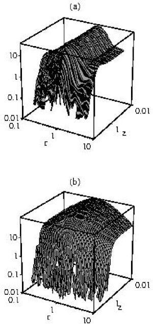
FIG. 1.: The two point correlation function $C_{11}(z,r)=k^{4}\sqrt{tt^{\prime}}\langle\Phi_{s}({\bf k},t)\Phi_{s}^{*}({\bf k},t^{\prime})\rangle$ is shown. Panel (a) represents the result from numerical simulations of the texture model; panel (b) shows the large-$N$ limit. For fixed $r$ the correlator is constant for $z<1$ and then decays. Note also the symmetry under $r\rightarrow 1/r$.

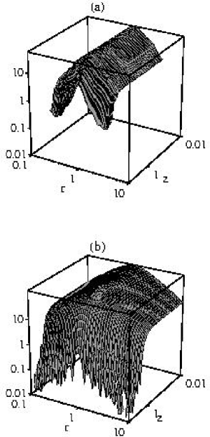
FIG. 2.: The same as Fig. 1 but for $C_{22}(z,r)=k^{4}\sqrt{tt^{\prime}}\langle\Psi_{s}({\bf k},t)\Psi_{s}^{*}({\bf k},t^{\prime})\rangle$.

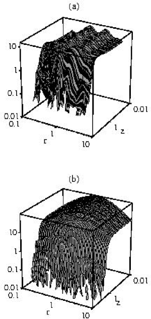
FIG. 3.: The unequal time correlator, $|C_{12}(z,r)|=k^{4}\sqrt{tt^{\prime}}|\langle\Phi_{s}({\bf k},t)\Psi_{s}^{*}({\bf k},t^{\prime})\rangle|$ is shown. Note that the $r\rightarrow 1/r$ symmetry is lost in this case.

In Fig. 4 we show $C_{ij}(z,r=1)$, and in Fig. 5 the ’constant’ of the Taylor expansion for $C_{ij}$ is given as a function of $r$, i.e., $C_{ij}(0,r)$.

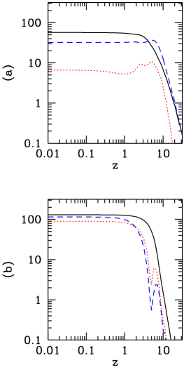
FIG. 4.: The correlators $C_{ij}(z,1)$ are shown. The solid, dashed and dotted lines represent $C_{22}~{},~{}C_{11}$ and $|C_{12}|$ respectively. Panel (a) is obtained from numerical simulations of the texture model and panel (b) shows the large-$N$ limit. A striking difference is that the large-$N$ value for $|C_{12}|$ is relatively well approximated by the perfectly coherent result $\sqrt{|C_{11}C_{22}|}$ while the texture curve for $|C_{12}|$ lies nearly a factor 10 lower.

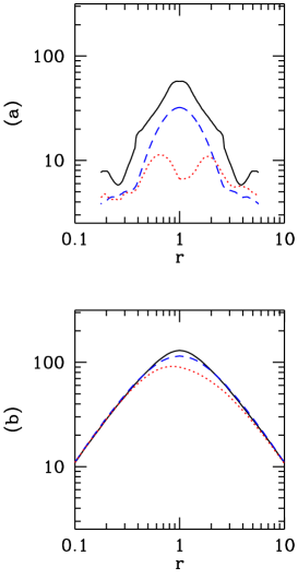
FIG. 5.: The correlators $C_{ij}(0,r)$ are shown in the same line styles as in Fig. 4, but for $z=0$ as function of $r=t^{\prime}/t$. The stronger decoherence of the texture model is even more evident here.

Vector perturbations are induced by $\mbox{\boldmath$\Sigma$}^{(s)}$ which is seeded by $\mbox{\boldmath$w$}^{(v)}$. Transversality and dimensional arguments require the correlation function to be of the form

$$\langle w_{i}^{(v)}({\bf k},t)w_{j}^{(v)*}({\bf k},t^{\prime})\rangle=\sqrt{tt^{\prime}}(k^{2}\delta_{ij}-k_{i}k_{j})W(z,r)~{}.$$ (133)

Again, as a consequence of causality, the function $W$ is analytic in $z^{2}$ (see [4]). The function $W(z,r)$ is plotted in Fig. 6. In Figs. 7 and 8 we graph $W(z,1)$ and $W(0,r)$.

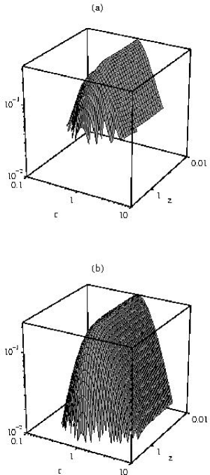
FIG. 6.: The vector correlator $W(z,r)$ is shown. The texture simulations, panel (a), and the large-$N$ limit, panel (b), give very similar results.

FIG. 7.: The vector correlator $W(z,1)$ is plotted. The solid line represents the texture simulations and the dashed line is the large-$N$ result. Up to a slight difference in amplitude, the two results are very similar.

FIG. 8.: The vector correlator $W(0,r)$ is shown. The solid line represents the texture simulations and the dashed line is the large-$N$ result. Also here, the two results are very similar. The ’wings’ visible in the texture curve are probably not due to a resolution problem but the beginning of oscillations.

Symmetry, transversality and tracelessness, together with statistical isotropy require the tensor correlator to be of the form (see [4])

$$\langle\tau^{(\pi)}_{ij}(t)\tau^{(\pi)*}_{lm}(t^{\prime})\rangle=$$ (137)

$${1\over\sqrt{tt^{\prime}}}T(z,r)[\delta_{il}\delta_{jm}+\delta_{im}\delta_{jl}-\delta_{ij}\delta_{lm}+k^{-2}(\delta_{ij}k_{l}k_{m}+$$

$$\delta_{lm}k_{i}k_{j}-\delta_{il}k_{j}k_{m}-\delta_{im}k_{l}k_{j}-\delta_{jl}k_{i}k_{m}-\delta_{jm}k_{l}k_{i})+$$

$$k^{-4}k_{i}k_{j}k_{l}k_{m}]~{}.$$

The functions $T(z,r)$ as well as $T(z,1)$ and $T(0,r)$ are shown in Figs. 9 to 11.

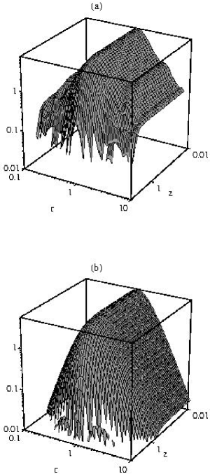
FIG. 9.: As Fig. 6, but for the tensor source function $T(z,r)$.

FIG. 10.: As Fig. 7, but for the tensor source function $T(z,1)$.

FIG. 11.: As Fig. 8, but for the tensor source function $T(0,r)$.

Clearly, all correlations between scalar and vector, scalar and tensor as well as vector and tensor perturbations have to vanish.

The scalar source correlation matrix $C$ and the functions $W$ and $T$ can be considered as kernels of positive hermitian operators in the variables $x=kt=zr^{1/2}$ and $x^{\prime}=kt^{\prime}=z/r^{1/2}$, which can be diagonalized.

$$C_{ij}(x,x^{\prime}) = \sum_{n}\lambda_{n}^{(S)}v_{in}^{(S)}(x)v_{jn}^{(S)\;*}(x^{\prime})~{},$$ (138)

$$W(x,x^{\prime}) = \sum_{n}\lambda_{n}^{(V)}v_{n}^{(V)}(x)v_{n}^{(V)\;*}(x^{\prime})~{},$$ (139)

$$T(x,x^{\prime}) = \sum_{n}\lambda_{n}^{(T)}v_{n}^{(T)}(x)v_{n}^{(T)\;*}(x^{\prime})~{},$$ (140)

where the series $\left(v_{in}^{(S)}\right)$, $\left(v_{n}^{(V)}\right)$ and $\left(v_{n}^{(T)}\right)$ are orthonormal series of eigenvectors (ordered according to the amplitude of the corresponding eigenvalue) of the operators $C$, $W$ and $T$ respectively for a given weight function $w$. We then have

$$\int C_{ij}(x,x^{\prime})v_{jn}^{(S)}(x^{\prime})w(x^{\prime})dx^{\prime} = \lambda_{n}^{(S)}v_{in}^{(S)}(x)~{},$$ (141)

$$\int W(x,x^{\prime})v_{n}^{(V)}(x^{\prime})w(x^{\prime})dx^{\prime} = \lambda_{n}^{(V)}v_{n}^{(V)}(x)~{},$$ (142)

$$\int T(x,x^{\prime})v_{n}^{(T)}(x^{\prime})w(x^{\prime})dx^{\prime} = \lambda_{n}^{(T)}v_{n}^{(T)}(x)~{}.$$ (143)

The eigenvectors and eigenvalues depend on the weight function $w$ which can be chosen to optimize the speed of convergence of the sums (138) to (140). In our models we found that scalar perturbations typically need 20 eigenvectors whereas vector and tensor perturbations need five to ten eigenvectors for an accuracy of a few percent (see Fig. 12).

FIG. 12.: The sum of the first few eigenfunctions of $T(x,x)$ is shown for two different weight functions, (a) logarithmic, $w=1/x$ and (b) linear, $w=1$. The first (long dashed), first and second (short dashed), first ten (dotted) and first thirty (solid) eigenfunctions are summed up. The open circles represent the full correlation function. Clearly, the eigenfunctions obtained by linear weighting converge much faster. Here we only show the equal time diagonal of the correlation matrix, but the same behavior is also found in the $C_{\ell}$ power spectrum which is sensitive to the full correlation matrix.

Inserting Eqs. (138) to (140) in Eq. (126), leads to

$$\langle X_{i}({\bf k},t_{0})X_{j}^{*}({\bf k},t_{0})\rangle=\sum_{n}\lambda_{n}X_{i}^{(n)}(kt_{0})X_{j}^{(n)*}(kt_{0})~{},$$ (144)

where $X_{i}^{(n)}(t_{0})$ is the solution of Eq. (122) with deterministic source term $v_{i}^{(n)}$.

$$X_{j}^{(n)}(t_{0},{\bf k})=\int_{t_{in}}^{t_{0}}dt{\cal G}(t_{0},t,{\bf k})_{jl}v_{l}^{(n)}(x,{\bf k})~{}.$$ (145)

For the CMB anisotropy spectrum this gives

$$C_{\ell}=\sum_{n}^{n_{S}}\lambda_{n}^{(S)}C_{\ell}^{(Sn)}+\sum_{n}^{n_{V}}\lambda_{n}^{(V)}C_{\ell}^{(Vn)}+\sum_{n}^{n_{T}}\lambda_{n}^{(T)}C_{\ell}^{(Tn)}~{}.$$ (146)

$C_{\ell}^{(\bullet n)}$ is the CMB anisotropy induced by the deterministic source $v_{n}$, and $n_{\bullet}$ is the number of eigenvalues which have to be considered to achieve good accuracy.

Instead of averaging over random solutions of Eq. (123), we can thus integrate Eq. (123) with the deterministic source term $v^{(n)}$ and sum up the resulting power spectra. The computational requirement for the determination of the power spectra of one seed model with given source term is thus on the order of $n_{S}$ inflationary models. This eigenvector method has first been applied in Ref. [5].

A source is called totally coherent[23, 13] if the unequal time correlation functions can be factorized. This means that only one eigenvector is relevant. A simple totally coherent approximation, which however misses some important characteristics of defect models, can be obtained by replacing the correlation matrix by the square root of the product of equal time correlators,

$$\langle\SS_{i}(t)\SS_{j}^{*}(t^{\prime})\rangle\rightarrow\pm\sqrt{\langle|\SS_{i}(t)|^{2}\rangle\langle|\SS_{j}(t^{\prime})|^{2}\rangle}~{}.$$ (147)

This approximation is exact if the source evolution is linear. Then the different ${\bf k}$ modes do not mix and the value of the source term at fixed ${\bf k}$ at a later time is given by its value at initial time multiplied by some transfer function, $\SS({\bf k},t)=\SS({\bf k},t_{in})T({\bf k},t,t_{in})$. In this situation, (147) becomes an equality and the model is perfectly coherent. Decoherence is due to the non-linearity of the source evolution which induces a ’sweeping’ of power from one scale into another. Different wave numbers ${\bf k}$ do not evolve independently.

It is interesting to note that the perfectly coherent approximation, (147), leaves open a choice of sign which has to be positive if $i=j$, but which is undetermined otherwise. According to Schwarz inequality the correlator $\langle\SS_{i}(t)\SS_{j}^{*}(t^{\prime})\rangle$ is bounded by

$$-\sqrt{\langle|\SS_{i}(t)|^{2}\rangle\langle|\SS_{j}(t^{\prime})|^{2}\rangle}\leq\langle\SS_{i}(t)\SS_{j}^{*}(t^{\prime})\rangle\leq$$ (149)

$$\sqrt{\langle|\SS_{i}(t)|^{2}\rangle\langle|\SS_{j}(t^{\prime})|^{2}\rangle}.$$

Therefore, for scales/variables for which the Greens function is not oscillating (e.g. Sachs Wolfe scales) the full result always lies between the ’anti-coherent’ (minus sign) and the coherent result. We have verified this behavior numerically.

The first evidence that Doppler peaks are suppressed in defect models has been obtained in the perfectly coherent approximation in Ref. [24]. In Fig. 13 we show the contributions to the $C_{\ell}$’s from more and more eigenvectors. A perfectly coherent model has only one non-zero eigenvalue.

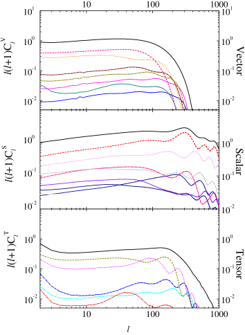
FIG. 13.: The scalar, vector and tensor contributions for the texture model of structure formation are shown. The dashed lines show the contributions from single eigenfunctions while the solid line represents the sum. Note that the single contributions to the scalar and tensor spectrum do show oscillations which are however washed out in the sum. (Vector perturbations do not obey a wave equation and thus do not show oscillations.)

A comparison of the full result with the totally coherent approximation is presented in Fig. 14.

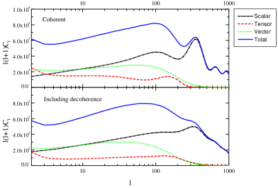
FIG. 14.: The $C_{\ell}$ power spectrum for the texture scenario is shown in the perfectly coherent approximation (top panel) and in the full eigenfunction expansion. Even in the coherent approximation, the acoustic peaks are not higher than the Sachs Wolfe plateau. Decoherence just washes out the structure but does not significantly damp the peaks.

There one sees that decoherence does smear out the oscillations present in the fully coherent approximation, and does somewhat damp the amplitude. Decoherence thus prevents the appearance of a series of acoustic peaks. The absence of power on this angular scale, however, is not a consequence of decoherence but is mainly due to the anisotropic stresses of the source which lead to perturbations in the geometry inducing large scale $C_{\ell}$’s (Sachs Wolfe), but not to density fluctuations. Large anisotropic stresses are also at the origin of vector and tensor fluctuations. Our results are in agreement with Refs. [24] and [5] but we disagree with Ref. [25], which has found acoustic peaks with an amplitude of about six in the coherent approximation.

In the real universe, perfect scaling of the seed correlation functions is broken by the radiation–matter transition, which takes place at the time of equal matter and radiation, $t_{eq}\simeq 20h^{-2}\Omega_{m}^{-1/2}$Mpc. The time $t_{eq}$ is an additional scale which enters the problem and influences the seed correlators. Only in a purely radiation or matter dominated universe are the correlators strictly scale invariant. This means actually that the $k$ dependence of the correlators $C$, $W$ and $T$ cannot really be cast into a dependence on $x$ and $x^{\prime}$, but that these functions depend on $t,t^{\prime}$ and $k$ in a more complicated way. We have to calculate and diagonalize the seed correlators for each wave number $k$ separately and the huge gain of dynamical range is lost as soon as scaling is lost.

In the actual case at hand, however, the deviation from scaling is weak, and most of the scales of interest to us enter the horizon only in the matter dominated regime. The behavior of the correlators in the radiation dominated era is of minor importance. To solve the problem, we calculate the correlator eigenvalues and eigenfunctions twice, in a pure radiation and in a pure matter universe and we interpolate the source term from the radiation to the matter epoch. Denoting by $\lambda_{m},v_{m}$ and $\lambda_{r},v_{r}$ a given pair of eigenvalue and eigenvector in a matter and radiation universe respectively, we choose as our deterministic source function

$$v(t) = y(t)\sqrt{\lambda_{r}}v_{r}(kt)+(1-y(t))\sqrt{\lambda_{m}}v_{m}(kt)$$ (150)

with, e.g., (151)

$$y(t) = {t_{eq}\over t+t_{eq}}~{}~{}\mbox{ or }~{}~{}~{}y(t)=\exp(-t/t_{eq})~{},$$ (152)

or some other suitable interpolation function. In Fig. 15 we show the results for scalar, vector and tensor perturbations respectively using purely radiation dominated era and from interpolated source terms.

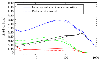
FIG. 15.: The scalar, vector, tensor and total $C_{\ell}$ power spectrum is shown from pure radiation sources and for an interpolated source. While the vector perturbations are somewhat higher in the radiation era, scalar and tensor perturbations are higher in the matter era and the sum is nearly unchanged.

Clearly the effect of the radiation dominated early state of the universe is relatively unimportant for the scales considered here. The difference between the pure matter era result and the interpolation is barely visible and thus not shown on the plot. This seems to be quite different for cosmic strings where the fluctuations in the radiation era are about twice as large as those in the matter era[26]. The radiation dominated era has very little effect on the key results which we are reporting here; namely the absence of acoustic peaks and the missing power on very large scales.

In models with cosmological constant, there is actually a second break of scale invariance at the matter–$\Lambda$ transition. There we proceed in the same way as outlined above. Since defects cease to scale and disappear rapidly in an exponentially expanding universe, the eigenvalues for the $\Lambda$ dominated universe all vanish.

E Initial conditions and numerical implementation

We numerically integrate our system of equations from redshift $z=10^{7}$ up to the present with the goal to have one percent accuracy up to $\ell\sim 1000$, for a given source term. We use the integration method described in Refs. [16] and [27]. We sample the interval $-5\leq\log_{10}kh^{-1}{\rm Mpc}\leq-0.75$ with minimum step size $\Delta\log_{10}=0.04$, for the scalar case and use a smoothing algorithm to suppress high frequency sampling noise. In order to save computing time, we start the integration of the $\sigma_{\ell}(k)$’s with $10$ harmonics, adding new harmonics in the course of the integration. We find that typically $\sim 40$ harmonics are sufficient for small $k$ values ($\log_{10}kh^{-1}{\rm Mpc}\stackrel{{\scriptstyle<}}{{\sim}}-3$), while for higher $k$ ($\log_{10}kh^{-1}{\rm Mpc}\stackrel{{\scriptstyle>}}{{\sim}}-1$), up to $\sim 1500$ harmonics for the scalar case, $\sim 200$ for the tensor case are needed to achieve the desired accuracy. Including more than $40$ harmonics for neutrinos corrects our results by less than one percent. We obtain $\Phi$ algebraically using Eq. (25). With this choice of variables we avoid the numerical difficulties present in conformal gauge [28], where $\Phi$ is determined by numerical integration.

The abundance of free electrons, $n_{e}$, is calculated following a standard recombination scheme [29] for $H$ and ${}^{4}He$, for a helium abundance by mass of 23%. At high redshift $z\geq 10^{5}$, the Thomson opacity is very large, and photons and baryons are tightly coupled. Due to the large Thomson drag term, Eqs.(47) and (57) become stiff and difficult to solve numerically. Therefore, in this limit we follow the method of Ref. [30], which is accurate to second order in $(\sigma_{T}n_{e})^{-1}$ (see also [28]). Assuming a standard inflationary model, we obtain a single scalar power spectrum in few minutes ($\sim 30$ seconds for the tensor case) on a PC class workstation, which differs by less than one percent from the $C_{\ell}$’s computed with other codes [31],[28].

Summing the scalar $C_{\ell}$’s from the largest $15$ eigenvectors ($5$ in the tensor case, $10$ for vector perturbations) typically reproduces the total sum to better than $5\%$ (see Fig. 13).

III The numerical simulations

As in previous work [7], we consider a spontaneously broken scalar field with O($N$) symmetry. We use the $\sigma$-model approximation, i.e., the equation of motion

$$\Box\beta-\left(\beta\cdot\Box\beta\right)\beta=0,$$ (153)

where $\beta$ is the rescaled field $\beta=\phi/\eta$.

We do not solve the equation of motion directly, but use a discretized version of the action [32]:

$$S=\int d^{4}\!x\,a^{2}(t)\left[\frac{1}{2}\partial_{\mu}\beta\cdot\partial^{\mu}\beta+\frac{\lambda}{2}\left(\beta^{2}-1\right)\right]\quad,$$ (154)

where $\lambda$ is a Lagrange multiplier which fixes the field to the vacuum manifold (this corresponds to an infinite Higgs mass). Tests have shown that this formalism agrees well with the complementary approach of using the equation of motion of a scalar field with Mexican hat potential and setting the inverse mass of the particle to the smallest scale that can be resolved in the simulation (typically of the order of $10^{-35}$ GeV), but tends to give better energy momentum conservation.

As we cannot trace the field evolution from the unbroken phase through the phase transition due to the limited dynamical range, we choose initially a random field at a comoving time $t=2\Delta x$. Different grid points are uncorrelated at all earlier times [33].

The use of finite differences in the discretized action as well as in the calculation of the energy momentum tensor introduce immediately strong correlations between neighboring grid points. This problem manifests itself in an initial phase of non-scaling behaviour, the length of which varies between $10\Delta x$ and $20\Delta x$, depending on the variable considered. It is very important to use results from the scaling regime only (cf. Fig. 16).

FIG. 16.: The ETCs $C_{11}(z,1)=\langle|\Phi|^{2}\rangle(kt)$ (panel a) and $C_{22}(z,1)=\langle|\Psi|^{2}\rangle(kt)$ (panel b) are shown for different times. In grid units the times are $t=4$ (dashed), $t=8$ (dotted), $t=12$ (long dashed), $t=16,~{}20$ (dash dotted, long dash dotted) and $t=24$ (solid). Clearly $C_{22}$ scales much sooner than $C_{11}$. To safely arrive in the scaling regime one has to wait until $t\sim 16$ and $C_{ij}(kt=0)$ is best determined at $t\geq 20$ but $kt<1$.

In order to reduce the time necessary to reach scaling and to improve the overall accuracy, we try to choose the finite differences in an optimal way. Our current code calculates all values in the center of each cubic cell defined by the lattice. The additional smoothing introduced by this improves energy-momentum conservation by several percent.

To calculate the unequal time correlator (UTC), the value of the observable under consideration is saved once scaling is reached at time $t_{c}$ (we checked this by using different correlation times) and then correlated at all following time steps. While there is some danger of contaminating the equal time correlator (ETC), which contributes most strongly to the $C_{\ell}$’s, with non-scaling sources, this method ensures that the constant for $kt\rightarrow 0$ is determined with maximal precision for the ETCs. This is very important as the constants $C_{ij}(0,1),~{}W(0,1)$ and $T(0,1)$ fix the relative size of scalar, vector and tensor contributions of the Sachs-Wolfe part and severely influence the resulting $C_{\ell}$’s. In contrast, the CMB spectrum seems quite stable under small variations of the shape of the UTCs.

The resulting UTCs are obtained numerically as functions of the variables $k$, $t$ and $t_{c}$ with $t\geq t_{c}$ and $t_{c}$ fixed. They are then linearly interpolated to the required range. We construct a hermitian $100\times 100$ matrix in $kt$ and $kt^{\prime}$, with the values of $kt$ chosen on a linear scale to maximize the information content, $0\leq kt\leq x_{\mathrm{m}ax}$. The choice of a linear scale ensures good convergence of the sum of the eigenvectors after diagonalization (see Fig. 12), but still retains enough data points in the critical region, ${\cal O}(x)=1$, where the correlators start to decay. In practice we choose as the endpoint $x_{\mathrm{m}ax}$ of the range sampled by the simulation the value at which the correlator decays by about two orders of magnitude, typically $x_{\mathrm{m}ax}\approx 40$. The eigenvectors that are fed into the Boltzmann code are then interpolated using cubic splines with the condition $v_{n}(kt)\rightarrow 0$ for $kt\gg x_{\mathrm{m}ax}$.

We use several methods to test the accuracy of the simulation: energy momentum conservation of the defects code is found to be better than 10% on all scales larger than about 4 grid units, as is seen in Fig. 17. A comparison with the exact spherically symmetric solution in non-expanding space [32] shows very good agreement.

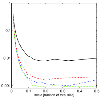
FIG. 17.: Energy momentum conservation of our numerical simulations is shown. The lines represent the sum of the terms which has to vanish if energy (solid) respectively momentum (dashed) is conserved, divided by the sum of the absolute value of these terms. The abscissa indicates the wavelength of the perturbation as fraction of the size of the entire grid.

The resulting CMB spectrum on Sachs Wolfe scales is consistent with the line of sight integration of Ref. [7]. Furthermore, the overall shape and amplitude of the unequal time correlators are quite similar to those found in the analytic large-$N$ approximation [35, 20, 4] (see Figs. 1 to 11). The main difference of the large-$N$ approximation is that there the field evolution, Eq. (153), is approximated by a linear equation. The non-linearities in the large-$N$ seeds which are due solely to the energy momentum tensor being quadratic in the fields, are much weaker than in the texture model where the field evolution itself is non-linear. Therefore, decoherence which is a purely non-linear effect, is expected to be much weaker in the large-$N$ limit. This is actually the main difference between the two models as can be seen in Fig. 18.

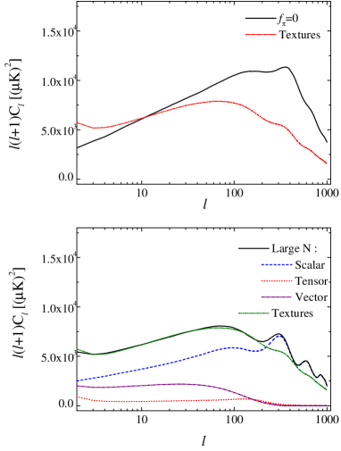
FIG. 18.: Top panel: the ${\it f_{\pi}}=0$ model. Bottom panel: The $C_{\ell}$ power spectrum is shown for the large-$N$ limit (bold line) and for the texture model. The main difference is clearly that the large-$N$ curve shows some acoustic oscillations which are nearly entirely washed out in the texture case.

IV Results and comparison with data

A CMB anisotropies

The $C_{\ell}$’s for the ’standard’ global texture model are shown in Fig. 14, bottom panel.

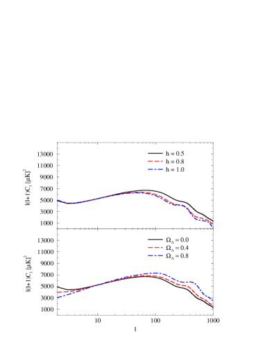
FIG. 19.: The $C_{\ell}$ power spectrum is shown for different values of cosmological parameters. In the top panel we choose $\Omega_{\Lambda}=0$, $\Omega_{CDM}=0.95$, $\Omega_{b}=0.05$ and vary $h$. In the bottom panel we fix $h=0.5$, $\Omega_{b}=0.05$ and vary $\Omega_{\Lambda}$. We only consider spatially flat universes, $\Omega_{0}=1$.

$\Omega_{\Lambda}$	$h$	$\epsilon$	$\sigma_{8}$
0.0	0.5	$(1.66\pm 0.17)10^{-5}$	0.24
0.0	0.8	$(1.67\pm 0.17)10^{-5}$	0.34
0.0	1.0	$(1.68\pm 0.17)10^{-5}$	0.44
0.4	0.5	$(1.64\pm 0.16)10^{-5}$	0.22
0.8	0.5	$(1.59\pm 0.16)10^{-5}$	0.16

TABLE I.: The value of the normalization constant $\epsilon$ and the fluctuation amplitude $\sigma_{8}$ are given for the different models considered. The error in $\epsilon$ comes from a best fit normalization to the full CMB data set. Cosmological parameters which are not indicated are identical in all models or given by $\Omega_{0}=\Omega_{cdm}+\Omega_{\Lambda}+\Omega_{b}=1$. We consider only spatially flat models with $\Omega_{b}=0.05$ and a helium fraction of 23%. The parameter choice indicated in the top line is referred to as standard texture model in the text.

Vector and tensor modes are found to be of the same order as the scalar component at COBE-scales. For the ’standard’ texture model we obtain $C_{10}^{(S)}:C_{10}^{(V)}:C_{10}^{(T)}\sim 0.9:1.0:0.3$, in good agreement with the predictions of Refs. [19], [5, 19, 17] and [4]. Due to tensor and vector contributions, even assuming perfect coherence (see Fig. 14, top panel), the total power spectrum does not increase from large to small scales. Decoherence leads to smoothing of oscillations in the power spectrum at small scales and the final power spectrum has a smooth shape with a broad, low isocurvature ’hump’ at $\ell\sim 100$ and a small residual of the first acoustic peak at $\ell\sim 350$. There is no structure of peaks at small scales. The power spectrum is well fitted by the following fourth-order polynomial in $x=\log\ell$:

$${\ell(\ell+1)C_{\ell}\over 110C_{10}}=1.5-2.6x+3.3x^{2}-1.4x^{3}+0.17x^{4}~{}.$$ (155)

The effect of decoherence is less important for the large-$N$ model, where oscillations and peaks are still visible (see Fig 18, bottom panel). This is due to the fact that the non-linearity of the large-$N$ limit is only in the quadratic energy momentum tensor. The scalar field evolution is linear in this limit[35], in contrast to the $N=4$ texture model. Since decoherence is inherently due to non-linearities, we expect it to be stronger for lower values of $N$. COBE normalization leads to $\epsilon=(0.92\pm 0.1)10^{-5}$ for the large-$N$ limit.

In Fig. 19 we plot the global texture $C_{\ell}$ power spectrum for different choices of cosmological parameters. The variation of parameters leads to similar effects like in the inflationary case, but with smaller amplitude. At small scales ($\ell\geq 200$), the $C_{\ell}$’s tend to decrease with increasing $H_{0}$ and they increase when a cosmological constant $\Omega_{\Lambda}=1-\Omega_{m}$ is introduced. Nonetheless, the amplitude of the anisotropy power spectrum at high $\ell$s remains in all cases on the same level like the one at low $\ell$s, without showing the substantial peak found in inflationary models. The absence of acoustic peaks is a stable prediction of global $O(N)$ models. The models are normalized to the full CMB data set, which leads to slightly larger values of the normalization parameter $\epsilon=4\pi G\eta^{2}$ than pure COBE normalization. In Table I we give the cosmological parameters and the value of $\epsilon$ for the models shown in Fig. 19.

In order to compare our results with current experimental data, we have selected a set of $31$ different anisotropy detections obtained by different experiments, or by the same experiment with different window functions and/or at different frequencies. Theoretical predictions and data of CMB anisotropies are usually compared by plotting the theoretical $C_{\ell}$ curve along with the CMB measurements converted to band power estimates. We do this in the top panel of Fig. 20. The data points show an increase in the anisotropies from large to smaller scales, in contrast to the theoretical predictions of the model. This fashion of presenting the data is surely correct, but lacks informations about the uncertainties in the theoretical model. Therefore we also compare the detected mean square anisotropy, $\Delta^{(Exp)}$ and the experimental 1-$\sigma$ error, $\Sigma^{(Exp)2}$, directly with the corresponding theoretical mean square anisotropy, given by

$$\Delta^{(Th)}={1\over{4\pi}}\sum_{\ell}(2\ell+1)C_{\ell}W_{\ell}~{},$$ (156)

where the window function $W_{\ell}$ contains all experimental details (chop, modulation, beam, etc.) of the experiment.

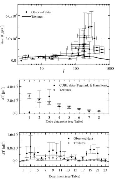
FIG. 20.: The $C_{\ell}$ spectrum obtained in the standard texture model is compared with data. In the top panel experimental results and the theoretical curve are shown as functions of $\ell$. In the two lower panels we indicate the value of each of the 31 experimental data points with 1-$\sigma$ error bars and the corresponding theoretical value with its uncertainty. The experiments corresponding to a given number are given in Table II. In the middle panel the 8 COBE data points are shown. In the bottom panel other experiments are presented.

The theoretical error in principle depends on the statistics of the perturbations. If the distribution is Gaussian, one can associate a sample/cosmic variance

$$\Sigma^{(Th)2}={1\over f}{1\over 8\pi^{2}}\sum_{\ell}(2\ell+1)W^{2}_{\ell}C^{2}_{\ell}~{},$$ (157)

where $f$ represents the fraction of the sky sampled by a given experiment.

Deviation from Gaussianity leads to an enhancement of this variance, which can be as large as a factor of $7$ (see [36]). Even if the perturbations are close to Gaussian (which has been found by simulations on large scales [7, 37]), the $C_{\ell}$’s, which are the squares of Gaussian variables, are non-Gaussian. This effect is, however only relevant for relatively low $\ell$s. Keeping this caveat in mind, and missing a more precise alternative, we nevertheless indicate the minimal, Gaussian error calculated according to (157). We add a $30\%$ error from the CMB normalization. The numerical seeds are assumed to be about 10% accurate.

In Table II, the detected mean square anisotropy, $\Delta^{(Exp)}$, with the experimental 1-$\sigma$ error are listed for each experiment of our data set. The corresponding sky coverage is also indicated. In Fig. 20 we plot these data points, together with the theoretical predictions for a texture model with $h=0.5$ and $\Omega_{\Lambda}=0$.

We find that, apart from the COBE quadrupole, only the Saskatoon experiment disagrees significantly, more than $1\sigma$, with our model. But also this disagreement is below $3\sigma$ and thus not sufficient to rule out the model. In the last column of Table II we indicate

$\displaystyle\chi_{j}^{2}=(\Delta_{j}^{(Th)}-\Delta_{j}^{(Exp)})^{2}/(\Sigma_{j}^{(Th)2}+\Sigma_{j}^{(Exp)2})$

for the $j$-th experiment, where the theoretical model is the standard texture model with $\Omega_{\Lambda}=0$ and $h=0.5$. The major discrepancy between data and theory comes from the COBE quadrupole. Leaving away the quadrupole, which can be contaminated and leads to a similar $\chi^{2}$ also for inflationary models, the data agrees quite well with the model, with the exception of three Saskatoon data points. Making a rough chi-square analysis, we obtain (excluding the quadrupole) a value $\chi^{2}=\sum_{j}\chi_{j}^{2}\sim 30$ for a total of 30 data points and one constraint. An absolutely reasonable value, but one should take into account that the experimental data points which we are considering are not fully independent. The regions of sky sampled by the Saskatoon and MSAM or COBE and Tenerife, for instance, overlap. Nonetheless, even reducing the degrees of freedom of our analysis to $N=25$, our $\chi^{2}$ is still in the range $(N-1)\pm{\sqrt{2}(N-1)}\sim 24\pm 7$ and hence still compatible with the data.

This shows that even assuming Gaussian statistics, the models are not convincingly ruled out from present CMB data. There is however one caveat in this analysis: A chi-square test is not sensitive to the sign of the discrepancy between theory and experiment. For our models the theoretical curve is systematically lower than the experiments. For example, whenever the discrepancy between theory and data is larger than $0.5\sigma$, which happens with nearly half of the data points (13), in all cases except for the COBE quadrupole, the theoretical value is smaller than the data. If smaller and larger are equally likely, the probability to have $12$ or more equal signs is $2(13+1)/2^{13}\simeq 3.4\times 10^{-3}$. This indicates that either the model is too low or that the data points are systematically too high. The number $0.003$ can however not be taken seriously, because we can easily change it by increasing our normalization on a moderate cost of $\chi^{2}$.

B Matter distribution

In Table I we show the expected variance of the total mass fluctuation $\sigma_{R}$ in a ball of radius $R=8h^{-1}$Mpc, for different choices of cosmological parameters. We find $\sigma_{8}=(0.44\pm 0.07)h$ (the error coming from the CMB normalization) for a flat model without cosmological constant, in agreement with the results of Ref. [5]. From the observed cluster abundance, one infers $\sigma_{8}=(0.50\pm 0.04)\Omega^{-0.5}$ [50] and $\sigma_{8}=0.59^{+0.21}_{-0.16}$ [51]. These results, which are obtained with the Press-Schechter formula, assume Gaussian statistics. We thus have to take them with a grain of salt, since we do not know how non-Gaussian fluctuations on cluster scales are in the texture model. According to Ref. [52], the Hubble constant lies in the interval $h\simeq 0.73\pm 0.06\pm 0.08$. Hence, in a flat CDM cosmology, taking into account the uncertainty of the Hubble constant, the texture scenario predicts a reasonably consistent value of $\sigma_{8}$.

As already noticed in Refs. [17] and [5], unbiased global texture models are unable to reproduce the power of galaxy clustering at very large scales, $\stackrel{{\scriptstyle>}}{{\sim}}20h^{-1}$ Mpc. In order to quantify this discrepancy we compare our prediction of the linear matter power spectrum with the results from a number of infrared ([53],[54]) and optically-selected ([55], [56]) galaxy redshift surveys, and with the real-space power spectrum inferred from the APM photometric sample ([57]) (see Fig. 22). Here, cosmological parameters have important effects on the shape and amplitude of the matter power spectrum. Increasing the Hubble constant shifts the peak of the power spectrum to smaller scales (in units of $h/$Mpc), while the inclusion of a cosmological constant enhances large scale power.

We consider a set of models in $\Omega_{\Lambda}$ – $h$ space, with linear bias [58] as additional parameter. In Table III we report for each survey and for each model the best value of the bias parameter obtained by $\chi^{2}$-minimization. We also indicate the value of $\chi^{2}$ (not divided by the number of data points). The data points and the theoretical predictions are plotted in Fig. 21. Our bias parameter strongly depends on the data considered. This is not surprising, since also the catalogs are biased relative to each other.

Models without cosmological constant and with $h\sim 0.8$ only require a relatively modest bias $b\sim 1.3-3$. But for these models the shape of the power spectrum is wrong as can be seen from the value of $\chi^{2}$ which is much too large. The bias factor is in agreement with our prediction for $\sigma_{8}$. For example, our best fit for the IRAS data, for $h\sim 0.8$ is $b\sim 1.3$. With $\sigma_{8}^{IRAS}=(0.69\pm 0.05)$, this gives $\sigma_{8}\sim 0.48\pm 0.04$, compatible with the direct computation

Whether IRAS galaxies are biased is still under debate. Published values for the $\beta$ parameter, defined as $\beta=\Omega^{0.6}/b$, for IRAS galaxies, range between $\beta_{I}=0.9^{+0.2}_{-0.15}$ [59] and $\beta_{I}=0.5\pm 0.1$ [60]. Biasing of IRAS galaxies is also suggested by measurements of bias in the optical band. For example, Ref. [61] finds $\beta_{o}=0.40\pm 0.12$, in marginal agreement with [62], which obtains $\beta_{o}=0.35\pm 0.1$. A bias for IRAS galaxies is not only possible but even preferred in flat global texture models.

But also with bias, our models are in significant contradiction with the shape of the power spectrum at large scales. As the values of $\chi^{2}$ in Table III and Fig. 22 clearly indicate, the models are inconsistent with the shape of the IRAS power spectrum, and they can be rejected with a high confidence level. The APM data which has the smallest error bars is the most stringent evidence against texture models. Nonetheless, these data points are not measured in redshift space but they come from a de-projection of a $2-D$ catalog into $3-D$ space. This might introduce systematic errors and thus the errors of APM may be underestimated.

Models with a cosmological constant agree much better with the shape of the observed power spectra, the value of $\chi^{2}$ being low for all except the APM data. But the values of the bias factors are extremely high for these models. For example, IRAS galaxies should have a bias $b\sim 3-6$, resulting in $\sigma_{8}\leq 0.25$, and in a $\beta_{I}\leq 0.2$ which is too small, even allowing for big variances due to non-Gaussian statistics.

The power spectra for the large-$N$ limit and for the coherent approximation are typically a factor 2 to 3 higher (see Fig. 22), and the biasing problem is alleviated for these cases. For $\Omega_{\Lambda}=0$ we find $\sigma_{8}=0.57h$ for the large-$N$ limit and $\sigma_{8}=0.94h$ for the coherent approximation. This is no surprise since only one source function, $\Psi_{s}$, the analog of the Newtonian potential, seeds dark matter fluctuations and thus the coherence always enhances the unequal time correlator. The second inequality in (149) applies. The dark matter Greens function is not oscillating, so this enhancement translates directly into the power spectrum.

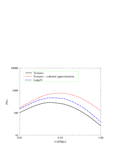
FIG. 21.: The dark matter power spectrum for the texture model (solid line) is compared with the coherent approximation (short dashed) and the large-$N$ limit (long dashed). The spectra are COBE normalized and the cosmological parameters are $\Omega_{\Lambda}=0~{},~{}h=0.5$.

Models which are anti-coherent in the sense defined in Section IID reduce power on Sachs-Wolfe scales and enhance the power in the dark matter. Anti-coherent scaling seeds are thus the most promising candidates which may cure some of the problems of global $O(N)$ models.

The simple analysis carried out here does not take into account the effects of non-linearities and redshift distortions. Redshift distortions in the texture case should be less important than in the inflationary case since the peculiar velocities are rather low (see next paragraph). Non-linearities typically set in at $k\geq 0.5h$Mpc^-1 and should not have a big effect on our main conclusions which come from much larger scales. Inclusion of these corrections will result in more small-scale power and in a broadening of the spectra, which even enhances the conflict between models and data. Furthermore, variations of other cosmological parameters, like the addition of massive neutrinos, hot dark matter, which is not considered here, will result in a change of the spectrum on small scales but will not resolve the discrepancy at large scales.

Nonetheless, scale dependent biasing may exist and lead to a non-trivial relation between the calculated dark matter power spectrum and the observed galaxy power spectrum. We are thus very reluctant to rule out the model by comparing two in principle different things, the relation of which is far from understood. Therefore we would prefer to reject the models on the basis of peculiar velocity data, which is more difficult to measure but most certainly not biased.

FIG. 22.: Matter Power spectrum: comparison between data and theory. References are in the text. Data set courtesy of M. S. Vogeley [65].

C Bulk velocities

To get a better handle on the missing power on 20 to 100$h^{-1}$Mpc, we investigate the velocity power spectrum which is not plagued by biasing problems. The assumption that galaxies are fair tracers of the velocity field seems to us much better justified, than to assume that they are fair tracers of the mass density. We therefore test our models against peculiar velocity data. We use the data by Ref. [63] which gives the bulk flow

$$\sigma^{2}_{v}(R)={H_{0}^{2}\Omega_{m}^{1.2}\over{2\pi^{2}}}\int P(k)W(kR)dk~{},$$ (158)

in spheres of radii $R=10$ to $60h^{-1}$Mpc. These data are derived after reconstructing the $3-$dimensional velocity field with the POTENT method (see [63] and references therein).

As we can see from Table IV, the COBE normalized texture model predicts too low velocities on large scales when compared with POTENT results. Recent measurements of the bulk flow lead to somewhat lower estimates like $\sigma_{v}(R)\sim(230\pm 90)$ at $R=60h^{-1}$Mpc ([64]), but still a discrepancy of about a factor of $2$ in the best case remains.

Including a cosmological constant helps at large scales, but decreases the velocities on small scales.

If the observational bulk velocity data is indeed reliable (there are some doubts about this[66]), all global $O(N)$ models are ruled out.

V Conclusions

We have developed a self contained formalism to determine CMB anisotropies and other power spectra for models with causal scaling seeds. We have applied it to global $O(N)$ models which contain global monopoles and texture. Our main results can be summarized as follows:

• Global $O(N)$ models predict a flat spectrum (Harrison-Zeldovich) of CMB anisotropies on large scales which is in good agreement with the COBE results. Models with vanishing cosmological constant and a large value of the Hubble parameter give $\sigma_{8}\sim 0.4$ to $0.5$ which is reasonable.

• Independent of cosmological parameters, these models do not exhibit pronounced acoustic peaks in the CMB power spectrum.

• The dark matter power spectrum from global $O(N)$ models with $\Omega_{\Lambda}=0$ has reasonable amplitude but does not agree in its shape with the galaxy power spectrum, especially on very large scales $>20h^{-1}$Mpc.

• Models with considerable cosmological constant agree relatively well with the shape of the galaxy power spectrum, but need very high bias $b\sim 4-6$ even with respect to IRAS galaxies.

• The large scale bulk velocities are by a factor of about 3 to 5 smaller than the value inferred from [63].

In view of the still considerable errors in the CMB data (see Fig. 20), and the biasing problem for the dark matter power spectrum, we consider the last argument as the most convincing one to rule out global $O(N)$ models. Even if velocity data is still quite uncertain, observations generally agree that bulk velocities on the scale of $50h^{-1}$Mpc are substantially larger than the (50 – 70)km/s obtained in texture models.

However, all our constraints have been obtained assuming Gaussian statistics. We know that global defect models are non-Gaussian, but we have not investigated how severely this influences the above conclusions. Such a study, which we plan for the future, requires detailed maps of fluctuations, the resolution of which is always limited by computational resources. Generically we can just say that non-Gaussianity can only weaken the above constraints.

Our results naturally lead to the question whether all scaling seed models are ruled out by present data. The main problem of the $O(N)$ model is the missing power at intermediate scales, $\ell\sim 300-500$ or $R\sim(20-100)h^{-1}{\rm Mpc}$. We have briefly investigated whether this problem can be mitigated in a scaling seed model without vector and tensor perturbations. In this case, also scalar anisotropic stresses are reduced by causality requirements (see Ref. [4]), and the compensation mechanism mentioned in Section II is effective. For simplicity, we analyze a model with purely scalar perturbations and no anisotropic stresses at all, $f_{\pi}=0$. The seed function $\Phi_{s}$ is taken from the texture model (numerical simulations) and we set $\Psi_{s}=-\Phi_{s}$. The resulting CMB anisotropy spectrum is shown in Fig. 18, top panel. A smeared out acoustic peak with an amplitude of about $2.2$ does indeed appear in this model. This is mainly due to the fact that fluctuations on large scales are smaller in this model, as is also evident from the higher value of $\epsilon=(2.2\pm 0.2)\times 10^{-5}$. But also here, the dark matter density fluctuations and bulk velocities are substantially lower than observed galaxy density fluctuations or the POTENT bulk flows.

Clearly, this simple example is not sufficient and a more thorough analysis of generic scaling seed models is presently under investigation. So far it is just clear that contributions from vector and tensor perturbations are severely restricted.
Acknowledgment
It is a pleasure to thank Andrea Bernasconi, Paolo de Bernardis, Roman Juszkiewicz, Mairi Sakellariadou, Paul Shellard, Andy Yates and Marc Davis for stimulating discussions. Our Boltzmann code is a modification of a code worked out by the group headed by Nicola Vittorio. We also thank Michael Vogeley who provided us with the galaxy power spectra shown in our figures. The numerical simulations have been performed at the Swiss super computing center CSCS. This work is partially supported by the Swiss National Science Foundation.

Experiment	Data point	$\Delta T^{2}(\mu K)^{2}$	$+(\mu K)^{2}$	$-(\mu K)^{2}$	Sky Coverage	Reference	$\chi^{2}_{j}$
COBE1	1	25.2	183	25.2	0.65	[38]	125.29
COBE2	2	212	126	128	0.65	[38]	0.02
COBE3	3	256	96.5	96.9	0.65	[38]	0.49
COBE4	4	105.5	48.3	48.2	0.65	[38]	0.74
COBE5	5	101.9	26.5	26.4	0.65	[38]	0.1
COBE6	6	63.4	19.11	18.9	0.65	[38]	1.11
COBE7	7	39.6	14.5	14.5	0.65	[38]	2.55
COBE8	8	42.5	12.7	12.8	0.65	[38]	0.04
ARGO Hercules	1	360	170	140	0.0024	[39]	0.001
MSAM93	2	4680	4200	2450	0.0007	[40]	0.74
MSAM94	3	4261	4091	2087	0.0007	[41]	0.51
MSAM94	4	1960	1352	858	0.0007	[41]	0.01
MSAM95	5	8698	6457	3406	0.0007	[42]	1.47
MSAM95	6	5177	3264	1864	0.0007	[42]	0.30
MAX HR	7	2430	1850	1020	0.0002	[43]	0.001
MAX PH	8	5960	5080	2190	0.0002	[43]	0.41
MAX GUM	9	6580	4450	2320	0.0002	[43]	0.73
MAX ID	10	4960	5690	2330	0.0002	[43]	0.17
MAX SH	11	5740	6280	2900	0.0002	[43]	0.25
Tenerife	12	3975	2855	1807	0.0124	[44]	0.64
South Pole Q	13	480	470	160	0.005	[45]	0.52
South Pole K	14	2040	2330	790	0.005	[45]	0.01
Python	15	1940	189	490	0.0006	[46]	0.37
ARGO Aries	16	580	150	130	0.0024	[47]	0.78
Saskatoon	17	1990	950	630	0.0037	[48]	0.79
Saskatoon	18	4490	1690	1360	0.0037	[48]	3.83
Saskatoon	19	6930	2770	2140	0.0037	[48]	4.60
Saskatoon	20	6980	3030	2310	0.0037	[48]	4.01
Saskatoon	21	4730	3380	3190	0.0037	[48]	1.32
CAT1	22	934	403	232	0.0001	[49]	1.36
CAT2	23	577	416	238	0.0001	[49]	0.62

TABLE II.: The CMB anisotropy detections used in our analysis. The 3., 4. and 5. column denote the value of the anisotropy and the upper and lower 1-$\sigma$ errors respectively. The references are: Tegmark and Hamilton 1997 [38]; de Bernardis et al. 1994 [39]; Cheng et al. 1994 [40]; Cheng et al. 1996 [41]; Cheng et al. 1997 [42]; Tanaka et al. 1996 [43]; Gutierrez et al. 1997 [44]; Gundersen et al. 1993 [45]; Dragovan et al. 1993 [46]; Masi et al 1996 [47]; Netterfield et al. 1996 [48]; Scott et al. 1997 [49].

Catalog	$h$	$\Omega_{\Lambda}$	Best fit bias $b$	$\chi^{2}$	Data points
CfA2-SSRS2 101 Mpc	0.5	0.0	3.4	29	24
CfA2-SSRS2 101 Mpc	0.8	0.0	2.0	40	24
CfA2-SSRS2 101 Mpc	1.0	0.0	1.9	44	24
CfA2-SSRS2 101 Mpc	0.5	0.4	3.9	17	24
CfA2-SSRS2 101 Mpc	0.5	0.8	9.5	4	24
CfA2-SSRS2 130 Mpc	0.5	0.0	5.3	8	19
CfA2-SSRS2 130 Mpc	0.8	0.0	3.4	15	19
CfA2-SSRS2 130 Mpc	1.0	0.0	3.4	16	19
CfA2-SSRS2 130 Mpc	0.5	0.4	5.6	5	19
CfA2-SSRS2 130 Mpc	0.5	0.8	11.1	4	19
LCRS	0.5	0.0	3.0	71	19
LCRS	0.8	0.0	1.8	96	19
LCRS	1.0	0.0	1.6	108	19
LCRS	0.5	0.4	3.7	33	19
LCRS	0.5	0.8	8.7	40	19
IRAS	0.5	0.0	2.3	102	11
IRAS	0.8	0.0	1.3	131	11
IRAS	1.0	0.0	1.3	140	11
IRAS	0.5	0.4	2.8	70	11
IRAS	0.5	0.8	6.3	9	11
IRAS 1.2 Jy	0.5	0.0	4.2	56	29
IRAS 1.2 Jy	0.8	0.0	2.9	92	29
IRAS 1.2 Jy	1.0	0.0	2.9	99	29
IRAS 1.2 Jy	0.5	0.4	4.3	39	29
IRAS 1.2 Jy	0.5	0.8	6.7	28	29
APM	0.5	0.0	3.3	1350	29
APM	0.8	0.0	1.8	1500	29
APM	1.0	0.0	1.7	1466	29
APM	0.5	0.4	3.5	1461	29
APM	0.5	0.8	6.2	1500	29
QDOT	0.5	0.0	4.3	32	19
QDOT	0.8	0.0	2.9	44	19
QDOT	1.0	0.0	2.9	46	19
QDOT	0.5	0.4	4.3	25	19
QDOT	0.5	0.8	7.3	14	19

TABLE III.: Analysis of the matter power spectrum. In the first column the catalog is indicated. Cols. 2 and 3 specify the model parameters. In cols. 4 and 5 we give the bias parameter inferred by $\chi^{2}$ minimization as well as the value of $\chi^{2}$. Col. 6 shows the number of ’independent’ data points assumed in the analysis.

R	$\sigma_{v}$ (R)	$\Delta_{v}$	$h=0.5$	$h=1.0$	$\Omega_{\Lambda}=0.8$
10	494	170	145	205	86
20	475	160	100	134	78
30	413	150	80	98	70
40	369	150	67	78	65
50	325	140	57	65	61
60	300	140	50	56	57

TABLE IV.: Bulk velocities: Observational data from [63] and theoretical predictions. $\Delta_{v}$ estimates the observational uncertainty. The uncertainties on the theoretical predictions are around $\sim 30\%$. The models $\Omega_{\Lambda}=0$ with $h=0.5$ and $h=1$ as well as $\Omega_{\Lambda}=0.8,~{}h=0.5$ are investigated.

A Complete definitions of gauge-invariant perturbation variables

In this Appendix we give precise definitions of all the gauge-invariant perturbation variables used in this paper. These definitions, their geometrical interpretation and a short derivation of the perturbation equations can be found in [9, 13]. We restrict the analysis to the spatially flat case, $K=0$. We define the perturbed metric by

$$g=\bar{g}+a^{2}h~{},$$ (A1)

where $\bar{g}$ denotes the standard Friedmann background, $a$ is the scale factor and $h$ denotes the metric perturbation.

1 Scalar perturbations

Scalar perturbations of the metric are of the form

$$h^{(S)} = -2A(dt)^{2}+2iBk_{j}dtdx^{j}+2(H_{L}+{1\over 3}H_{T})\delta_{ij}dx^{i}dx^{j}$$ (A3)

$$-2k^{-2}H_{T}k_{i}k_{j}dx^{i}dx^{j}~{}.$$

Computing the perturbation of the Ricci curvature scalar and the shear of the equal time slices, we obtain

$$\delta\mbox{\boldmath$R$}=4a^{-2}k^{2}{\cal R}~{}\mbox{ , with }~{}~{}~{}{\cal R}=H_{L}+{1\over 3}H_{T}\;,$$ (A4)

$$K^{\mathrm{(}aniso)} = a\sigma({k_{i}k^{j}\over k^{2}}-{1\over 3}\delta_{i}^{j})dx^{i}\otimes\partial_{j}~{},$$ (A5)

with (A6)

$$\sigma = k^{-1}\dot{H}_{T}-B~{}.$$ (A7)

The Bardeen potentials are the combinations

$$\Phi = {\cal R}-(\dot{a}/a)k^{-1}\sigma$$ (A8)

$$\Psi = A-k^{-1}[(\dot{a}/a)\sigma-\dot{\sigma}]\;.$$ (A9)

They are invariant under infinitesimal coordinate transformations (gauge transformations).

To define perturbations of the most general energy momentum tensor, we introduce the energy density $\rho$ and the energy flux $u$ as the time-like eigenvalue and normalized eigenvector of $T^{\mu}_{\nu}$,

$\displaystyle T_{\mu}^{\;\;\nu}u^{\mu}=-\rho u^{\nu}\;\;,\;\;u^{2}=-1\;.$

We then define the perturbations in the energy density and energy velocity field by

$$\rho=\overline{\rho}(1+\delta)\;\;,$$ (A10)

$$u=u^{0}\partial_{t}+u^{i}\partial_{i}~{};$$ (A11)

$u^{0}$ is fixed by the normalization condition, $u^{0}=a^{-1}(1-A)$. In the 3–space orthogonal to $u$ we define the stress tensor by

$$\tau^{\mu\nu}\equiv P^{\mu}_{~{}~{}\alpha}P^{\nu}_{~{}~{}\beta}T^{\alpha\beta}~{},$$ (A12)

where $P=u\otimes u+g$ is the projection onto the sub–space of $T{\cal M}$ normal to $u$. It is

$\displaystyle\tau^{0}_{0}=\tau^{0}_{i}=\tau^{i}_{0}=0~{}.$

The perturbations of pressure and anisotropic stresses can be parameterized by

$$\tau_{i}^{\;j}=\bar{p}[(1+\pi_{L})\delta_{i}^{\;j}+\pi_{i}^{\;\;j}]~{}~{}\mbox{ , with }~{}\pi^{i}_{i}=0\;.$$ (A13)

For scalar perturbations we set

$$u^{0} = (1-A)\;,\;{u^{(S)j}\over u^{0}}=-i{k^{j}\over k}v$$

and

$$\pi^{(S)i}_{~{}j} = (-k^{-2}k^{i}k_{j}+{1\over 3}\delta^{i}_{~{}j})\Pi~{}.$$

Studying the behavior of these variables under gauge transformations, one finds that the anisotropic stress potential $\Pi$ is gauge invariant. A gauge invariant velocity variable is the shear of the velocity field,

$$\sigma^{(Sm)}_{ij}=(k^{-2}k_{i}k_{j}-{1\over 3}\delta_{ij}a^{3}V\mbox{ , ~{}with }~{}~{}V=v-k^{-1}\dot{H}_{T}.$$ (A14)

There are several different useful choices of gauge invariant density perturbation variables,

$$D_{s} = \delta+3(1+w)(\dot{a}/a)k^{-1}\sigma$$ (A15)

$$D_{g} = \delta+3(1+w){\cal R}=D_{s}+3(1+w)\Phi$$ (A16)

$$D = D_{s}+3(1+w)(\dot{a}/a)k^{-1}V\;.$$ (A17)

In this work we mainly use $D_{g}$. Here $w=p/\rho$ denotes the enthalpy. Clearly, these matter variables can be defined for each matter component separately. For ideal fluids like CDM or the baryon photon fluid long before decoupling, anisotropic stresses vanish and $\pi_{L}=(c_{s}^{2}/w)\delta$, where $c_{s}$ is the adiabatic sound speed.

Also scalar perturbations of the photon brightness, $\iota^{(S)}$ are not gauge invariant. It has been show[9] that the combination

$${\cal M}^{(S)}=\iota^{(S)}+4{\cal R}+4ik^{-1}n^{j}k_{j}\sigma$$ (A18)

is gauge invariant. This is the variable which we use here. In other work[67] the gauge invariant variable $\Theta\equiv{\cal M}+\Phi$ has been used. Since $\Phi$ is independent of the photon direction ${\bf n}$ this difference in the definition shows up only in the monopole, $C_{0}$. But clearly, as can be seen from Eq. (A18), also the dipole, $C_{1}$, is gauge dependent.

The brightness perturbation of the neutrinos is defined the same way and will not be repeated here.

2 Vector perturbations

Vector perturbations of the metric are of the form

$$h^{(V)}=2B_{j}dx^{j}dt+ik^{-1}(k_{l}H_{j}+k_{j}H_{l})dx^{l}dx^{j}~{},$$ (A19)

where $\bf B$ and $\bf H$ are transverse vector fields. The simplest gauge invariant variable describing the two vectorial degrees of freedom of metric perturbations is $\Sigma$,

$$\Sigma_{j}=k^{-1}\dot{H}_{j}-B_{j}~{}.$$ (A20)

Vectorial anisotropic stresses are gauge invariant. They are of the form

$$\pi_{lj}^{(V)}=ik^{-1}(k_{j}\Pi_{l}+k_{l}\Pi_{j})~{}.$$ (A21)

The vector degrees of freedom of the velocity field are cast in the vorticity

$$u_{l:j}-u_{j;l} = ia(k_{j}\omega_{l}-k_{l}\omega_{j})$$ (A22)

with $$\omega_{j}=v_{j}-B_{j}~{}.$$ (A23)

Vector perturbations of the photon brightness are gauge-invariant. To maintain a consistent notation, we denote them by ${\cal M}^{(V)}$.

3 Tensor perturbations

We define tensor perturbations of the metric by

$$h^{(T)}=2H_{ij}dx^{i}dx^{j}~{},$$ (A24)

where $H_{ij}$ is a traceless transverse tensor field.

The only tensor perturbations of the energy momentum tensor are anisotropic stresses,

$$\pi_{lj}^{(T)}=\Pi_{lj}~{}.$$ (A25)

Tensor perturbations of the photon brightness are denoted ${\cal M}^{(T)}$.

Clearly, all tensor perturbations are gauge-invariant (there are no tensor type gauge transformations).

B The CMB anisotropy power spectrum

Here we derive in some detail Eqs. (92), (108) and (120).

CMB anisotropies are conveniently expanded in spherical harmonics: $\delta T({\bf n})/T_{0}=\sum_{lm}a_{lm}Y_{m}^{l}({\bf n})$. The coefficients $a_{lm}$ are random variables with zero mean and rotationally invariant variances, $C_{\ell}\equiv\langle\mid a_{lm}\mid^{2}\rangle$. The mean (over the ensemble) correlation function of the anisotropy pattern has the standard expression:

$$\left\langle{\delta T\over T_{0}}({\bf n}_{1}){\delta T\over T_{0}}({\bf n}_{2})\right\rangle={1\over 4\pi}\sum_{\ell}(2\ell+1){C_{\ell}}P_{\ell}(\cos\theta)$$ (B1)

where $\cos\theta={\bf n}_{1}\cdot{\bf n}_{2}$. To find Eq. (92) we use the Fourier transform normalization

$$\hat{f}({\bf k})={1\over V}\int f({\bf x})\exp(i{\bf k}\cdot{\bf x})d^{3}x~{},$$ (B2)

with some normalization volume $V$. Assuming that ensemble average can be replaced by volume average then implies

$$\left\langle{\delta T\over T_{0}}({\bf n}_{1}){\delta T\over T_{0}}({\bf n}_{2})\right\rangle~{}=~{}{1\over V}\int d^{3}x{\delta T\over T_{0}}({\bf x},{\bf n}_{1}){\delta T\over T_{0}}({\bf x},{\bf n}_{2})$$ (B4)

$$=~{}{1\over(2\pi)^{3}}\int d^{3}k{\delta T\over T_{0}}({\bf k},{\bf n}_{1}){\delta T\over T_{0}}({\bf k},{\bf n}_{2})~{}.$$

Inserting our ansatz (74) for ${\delta T\over T_{0}}={1\over 4}{\cal M}$, and using the addition theorem for spherical harmonics, we have

$$\left\langle{\delta T\over T_{0}}({\bf n}_{1}){\delta T\over T_{0}}({\bf n}_{2})\right\rangle=$$ (B8)

$${1\over 8\pi}\sum_{\ell,\ell^{\prime},m,m^{\prime}}(-1)^{(\ell-\ell^{\prime})}Y_{\ell m}(n_{1})Y^{*}_{\ell^{\prime}m^{\prime}}(n_{2})\times$$

$$\int k^{2}dkd\Omega_{\hat{{\bf k}}}Y_{\ell m}^{*}(\hat{{\bf k}})Y_{\ell^{\prime}m^{\prime}}(\hat{{\bf k}})\langle\sigma_{\ell}\sigma^{*}_{\ell^{\prime}}\rangle(k)~{}=~{}$$

$$={1\over 32\pi^{2}}\sum_{\ell}(2\ell+1)P_{\ell}({\bf n}_{1}\cdot{\bf n}_{2})\int k^{2}dk\langle\sigma_{\ell}\sigma^{*}_{\ell}\rangle(k)~{},$$

from which we can read of Eq. (92).

For vector and tensor fluctuations, the ansatz (96) and (112) must be taken into account. With the same manipulations as above the correlation function of CMB anisotropies induced by vector modes reads:

$$\left\langle{\delta T\over T_{0}}({\bf n}_{1}){\delta T\over T_{0}}({\bf n}_{2})\right\rangle=$$ (B10)

$${1\over{128\pi^{3}}}\int d^{3}k\sum_{\ell 1\ell 2}\Pi_{\ell 1,\ell 2}({\bf k},{{\bf n}^{\prime}}_{1},{{\bf n}^{\prime}}_{2})P_{\ell 1}({\mu^{\prime}}_{1})P_{\ell 2}({\mu^{\prime}}_{2})$$

where the primes indicate that the quantity is considered in the reference system where ${\bf k}$ is parallel to the $z$ axis and ([68],[16])

$$\Pi_{\ell 1,\ell 2} = (-i)^{(\ell 1-\ell 2)}(2\ell_{1}+1)(2\ell_{2}+1)$$ (B14)

$$\sqrt{(1-(\mu^{\prime}_{2})^{2})(1-(\mu^{\prime}_{2})^{2})}\times$$

$$[\langle\sigma^{(V)}_{1,\ell 1}\sigma_{1,\ell 2}^{(V)*}\rangle\cos(\phi^{\prime}_{1})\cos(\phi^{\prime}_{2})+$$

$$+\langle\sigma_{2,\ell 1}^{(V)}\sigma_{2,\ell 2}^{(V)*}\rangle\sin(\phi^{\prime}_{1})\sin(\phi^{\prime}_{2})]~{}.$$

Assuming statistical isotropy which implies

$\displaystyle\langle|\sigma_{1,\ell}^{(V)}|^{2}\rangle=\langle|\sigma_{2,\ell}^{(V)}|^{2}\rangle~{}~{}~{}\mbox{ and }~{}~{}~{}\langle\sigma_{1,\ell}^{(V)}\sigma_{2,\ell}^{*(V)}\rangle=0~{},$

we obtain

$$\left\langle{{\delta T({\bf n}_{1})}\over{T_{0}}}{{\delta T({\bf n}_{2})}\over{T_{0}}}\right\rangle=$$ (B17)

$${1\over{128\pi^{3}}}\sum_{\ell 1\ell 2}(2\ell_{1}+1)(2\ell_{2}+1)(-i)^{(\ell 1-\ell 2)}\times$$

$$\int\Upsilon({{\bf n}^{\prime}}_{1},{{\bf n}^{\prime}}_{2})\langle\sigma_{1,\ell 1}^{(V)}\sigma_{1,\ell 2}^{(V)*}\rangle P_{\ell 1}({\mu^{\prime}}_{1})P_{\ell 2}({\mu^{\prime}}_{2})d^{3}k~{},$$

where

$$\Upsilon={{{\bf n}_{1}}\cdot{{\bf n}_{2}}-\mu^{\prime}_{1}\mu^{\prime}_{2}}~{}.$$ (B18)

Using the recursion formula for Legendre polynomials and the addition theorem for spherical harmonics, we find after some manipulations

$$C_{\ell}^{(V)}={\ell(\ell+1)\over{8\pi}}\int k^{2}dk{{\langle|\sigma^{(V)}_{1,\ell+1}(t_{0},k)+\sigma^{(V)}_{1,\ell-1}(t_{0},k)|^{2}\rangle}\over{(2\ell+1)^{2}}}~{}.$$ (B19)

For the correlation function of the CMB anisotropies from tensor modes our ansatz (112) gives

$${\left\langle{\delta T\over T_{0}}({\bf n}_{1}){\delta T\over T_{0}}({\bf n}_{2})\right\rangle}=$$ (B21)

$${1\over{128\pi^{3}}}\int{\sum_{\ell 1\ell 2}\Pi_{\ell 1,\ell 2}(k,{{\bf n}^{\prime}}_{1},{{\bf n}^{\prime}}_{2})P_{\ell 1}({\mu^{\prime}}_{1})P_{\ell 2}({\mu^{\prime}}_{2})d^{3}k}$$

with

$$\Pi_{\ell 1,\ell 2} = (-i)^{\ell 1-\ell 2}(2\ell 1+1)(2\ell 2+1)(1-(\mu^{\prime}_{1})^{2})\times$$ (B24)

$$(1-(\mu^{\prime}_{2})^{2})[\langle\sigma^{(T)}_{\times,\ell 1}\sigma_{\times,\ell 2}^{(T)*}\rangle\cos(2\phi^{\prime}_{1})\cos(2\phi^{\prime}_{2})+$$

$$+\langle\sigma_{+,\ell 1}^{(T)}\sigma_{+,\ell 2}^{(T)*}\rangle\sin(2\phi^{\prime}_{1})\sin(2\phi^{\prime}_{2})].$$

Here, statistical isotropy leads to

$$\left\langle{\delta T({\bf n}_{1})\over T_{0}}{\delta T({\bf n}_{2})\over T_{0}}\right\rangle=$$ (B27)

$${1\over 128\pi^{3}}\sum_{\ell 1\ell 2}(2\ell_{1}+1)(2\ell_{2}+1)(-i)^{(\ell 1-\ell 2)}\times$$

$$\int\Upsilon({\bf n}^{\prime}_{1},{\bf n}^{\prime}_{2})\langle\sigma_{+,\ell 1}^{(T)}\sigma_{+,\ell 2}^{(T)*}\rangle P_{\ell 1}(\mu^{\prime}_{1})P_{\ell 2}(\mu^{\prime}_{2})d^{3}k$$

where

$$\Upsilon=[2({{\bf n}_{1}}\cdot{{\bf n}_{2}}-\mu^{\prime}_{1}\mu^{\prime}_{2})^{2}-(1-(\mu^{\prime}_{1})^{2})(1-(\mu^{\prime}_{2})^{2})]~{}.$$ (B28)

With straightforward but somewhat cumbersome manipulations, applying the recursion formula for Legendre polynomials and the addition theorem for spherical harmonics, we then obtain

$${C^{(T)}_{\ell}}={1\over 8\pi}{(\ell+2)!\over(\ell-2)!}\int_{0}^{\infty}{\mid{\Sigma^{(T)}_{\ell}(k)}\mid^{2}\over(2\ell+1)^{2}}k^{2}dk~{},$$ (B29)

with

$$\Sigma^{(T)}_{\ell}={{\sigma^{(T)}_{{\epsilon},\ell-2}}\over{2\ell-1}}-{{2{(2\ell+1)\sigma^{(T)}_{{\epsilon},\ell}}}\over{(2\ell-1)(2\ell+3)}}+{{\sigma^{(T)}_{{\epsilon},\ell+2}}\over{{2\ell+3}}}~{}.$$ (B30)

The formulas (B8),(B19) and (B29) are used to determine the CMB anisotropy spectrum.

REFERENCES

-
[1]
See the web sites:
http://astro.estec.esa.nl/SA-general
/Projects/Planck/
and http://map.gsfc.nasa.gov/ - [2] W. Hu, N. Sugiyama and J. Silk, Nature 386, 37 (1995).
- [3] R. Durrer, M. Kunz, C. Lineweaver and M. Sakellariadou, Phys. Rev. Lett. 79, 5198 (1997).
- [4] R. Durrer and M. Kunz, Phys, Rev. D 57, R3199 (1998).
- [5] U. Pen, U. Seljak and N. Turok, Phys. Rev. Lett. 79, 1611 (1997).
- [6] P.P. Avelino, E.P.S. Shellard, J.H.P. Wu and B. Allen, Phys. Rev. Lett., in print (archived under astro-ph/9712008) (1998).
- [7] R. Durrer and Z. Zhou, Phys. Rev. D 53, 5394 (1996).
- [8] R. Durrer, Phys. Rev. D 42, 2533 (1990).
- [9] R. Durrer, Fund. of Cosmic Physics 15, 209 (1994).
- [10] J.M. Stewart and M. Walker, Proc. R. Soc. London A341, 49 (1974).
- [11] J. Bardeen, Phys. Rev. D 22, 1882 (1980).
- [12] H. Kodama and M. Sasaki, Prog. Theor. Phys. Suppl. 78, 1 (1984).
- [13] R. Durrer and M. Sakellariadou, Phys. Rev. D 56, 4480 (1997).
- [14] C. Cheung and J. Magueijo, Phys. Rev. D 56, 1982 (1997).
- [15] J.P. Uzan, N. Deruelle and N. Turok, Phys. Rev. D 57, 7192 (1998).
- [16] A. Melchiorri and N. Vittorio, Polarization of the microwave background: Theoretical framework, in: Proceedings of the NATO Advanced Study Institute 1996 on the ”Cosmic Background Radiation”, Strasbourg, archived under astro-ph 9610029, (1996)
- [17] A. Albrecht, R. Battye and J. Robinson, Phys. Rev. Lett. 79, 4736 (1997).
- [18] A. Albrecht, D. Coulson, P.G. Ferreira and J. Magueijo, Phys. Rev. Lett. 76, 1413 (1996).
- [19] B. Allen et al., Phys. Rev. Lett. 79, 2624 (1997).
- [20] M. Kunz and R. Durrer, Phys. Rev. D 55, R4516 (1997).
- [21] C. Contaldi, M. Hindmarsh and J. Magueijo, preprint archived under astro-ph/9808201 (1998).
- [22] N. Turok and D. Spergel, Phys. Rev. Lett 66, 3093 (1991).
- [23] J. Magueijo, A. Albrecht, P.G. Ferreira and D. Coulson, Phys. Rev. D 54, 3727 (1996).
- [24] R. Durrer, A. Gangui and M. Sakellariadou, Phys. Rev. Lett. 76, 579 (1996).
- [25] R. Crittenden and N. Turok, Phys. Rev. Lett. 75, 2642 (1995).
- [26] P. Shellard, private communication (1998).
- [27] P. de Bernardis, A. Balbi, G. De Gasperis, A. Melchiorri and N. Vittorio, Astrophys. J. 480, 1 (1997).
- [28] C.P. Ma and E. Bertschinger, Astrophys. J. 455, 7 (1995).
- [29] B.J. Jones and R. Wyse, Astron. & Astrophys. 149, 144 (1985).
- [30] P.J.E. Peebles and J.T. Yu, Astrophys. J. 162, 815 (1970)
- [31] U. Seljak and M. Zaldarriaga, Astrophys. J. 496, 437 (1996).
- [32] U. Pen, D. Spergel and N. Turok, Phys Rev. D 49, 692 (1994).
- [33] W. P. Petersen and A. Bernasconi, CSCS Technical Report TR-97-06 (1997).
- [34] J. Borrill, private communication.
- [35] N. Turok and D. Spergel, Phys. Rev. Lett. 64, 2736 (1990).
- [36] X. Luo, Astrophys. J. 439, 517L (1995) .
- [37] B. Allen et al., Phys. Rev. Lett 77, 3061 (1996).
- [38] M. Tegmark and A. Hamilton, archived under astro-ph/9702019 (1997)
- [39] P. de Bernardis et al., Astrophys. J. 422, 33L (1994).
- [40] E.S. Cheng et al., Astrophys. J. 422, 40L (1994).
- [41] E.S. Cheng et al., Astrophys. J. 456, 71L (1996).
- [42] E.S. Cheng et al., ApJ488, 59L (1997).
- [43] S.T. Tanaka et al., Astrophys. J. 468, 81L (1996).
- [44] C. M. Gutierrez et al., Astrophys. J. 480, 83L (1997).
- [45] J.O. Gundersen et al., ApJ413, 1L (1993).
- [46] M. Dragovan et al., ApJ427, 67L (1993).
- [47] S. Masi et al., ApJ463, 47L (1996).
- [48] B. Netterfield et al., ApJ474, 47 (1997).
- [49] P.F. Scott at al., ApJ461, 1L (1996).
- [50] V.R. Eke, S. Cole and C.S. Frenk M.N.R.A.S. 282, 263E (1996).
- [51] A.R. Liddle, D. Lyth, H. Robeerts, P. Viana, M.N.R.A.S. 278, 644 (1996).
- [52] W. Freedman, J.R. Mould, R.C. Kennicut and B.F. Madore, archived under astro-ph/9801080 (1998).
- [53] K.B. Fisher, M. Davis, M.A. Strauss, A. Yahil and J.P. Huchra, M.N.R.A.S. 266, 50 (1994).
- [54] H. Tadros and G. Efstathiou, M.N.R.A.S., L45, 276 (1995).
- [55] L.N. Da Costa, M.S. Vogeley, M.J. Geller, J.P. Huchra and C. Park, Astrophys. J. 437, 1L (1994).
- [56] H. Lin et al., AAS, 185, 5608L (1994).
- [57] C.M. Baugh and G. Efstathiou, M.N.R.A.S., 265, 145 (1993).
- [58] N. Kaiser, Astrophys. J. 284, 9L (1984).
- [59] N. Kaiser, G. Efstathiou, R. Ellis, C.S. Frenk, A. Lawrence, M. Rowan-Robinson and W. Saunders, M.N.R.A.S. 252, 1 (1991).
- [60] J.A. Willick, S. Courteau, S.M. Faber, D. Burstein, A. Dekel and T. Kolatt, Astrophys. J. 457, 460 (1996).
- [61] J.A. Peacock, M.N.R.A.S. 284, 885P (1997).
- [62] E.J. Shaia, P.J.E. Peebles and R.B. Tully, Astrophys. J. 454, 15 (1995).
- [63] A. Dekel, Ann. Rev. of Astron. and Astrophys. 32, 371 (1994).
- [64] R. Giovanelli et al., preprint, archived under astro-ph/98707274 (1998).
- [65] M.S. Vogeley, to appear in ”Ringberg Workshop on Large-Scale Structure”, ed. D. Hamilton, (Kluwer, Amsterdam), archived under astro-ph/9805160 (1998).
- [66] M. Davis, private communication (1998).
- [67] W. Hu and N. Sugiyama, Phys. Rev. D 51, 2599 (1995), and references therein.
- [68] A. Kosowsky, Annals of Physics 246, 49 (1996).