Weak Lensing: Prospects for Parameter Estimation

Abstract

Weak lensing of galaxies by large scale structure can potentially measure cosmological quantities as precisely as the cosmic microwave background (CMB) though the relation between the observables and the fundamental parameters is more complex and degenerate, especially in the full space of adiabatic cold dark matter models considered here. We introduce a Fisher matrix analysis of the information contained in weak lensing surveys to address these issues and provide a simple means of estimating how survey propreties and source redshift uncertainties affect parameter estimation. We find that even if the characteristic redshift of the sources must be determined from the data itself, surveys on degree scales and above can significantly assist the CMB on parameters that affect the growth rate of structure.

1. Introduction

Weak lensing of faint galaxies by large scale structure can in principle provide precise constraints on the spectrum and evolution of mass fluctuations in the universe (Miralda-Escude 1991; Blandford et al 1991; Kaiser 1992). Given the same sky coverage, the statistical errors on these measurements should be as small as those from the cosmic microwave background (CMB). The main systematic errors are detector-based rather than astrophysical; though they currently present a great obstacle against detection, it is one that is in principle surmountable.

Because lensing convolves aspects of the spectrum of present-day mass fluctuations, their evolution, and the distribution of source galaxies, it is less clear how to translate precision in the observables into precision in the cosmological parameters. Previous work has focussed on a relatively small number of parameters such as the matter density and the present-day amplitude of the its power spectrum assuming a fixed functional form and a fixed distribution of sources (e.g. Jain & Seljak 1997; Bernardeau et al 1997; Kaiser 1998). Even so predictions depend strongly on prior assumptions for these parameters.

In this Letter, we introduce a Fisher information matrix approach to assess the ability of weak-lensing power spectrum measurements to determine cosmological parameters. The virtue of this approach is its ability to simply quantify how assumptions about the survey properties, parameter space, fiducial model and prior knowledge from other cosmological measurements affect parameter estimation. We study an 11 dimensional parameter space based on the adiabatic cold dark matter model and show that information from CMB anisotropy measurements can be used in lieu of large sky coverage in isolating several key cosmological parameters and measuring the redshift distribution of the sources.

We begin in §2 with the Fisher matrix formalism. In §3, we describe the parameterization of the cosmological model to which we apply this formalism in §4. We study the effect of the source sampling and distribution in §5 and summarize our conclusions in §6.

2. Fisher Matrix

By measuring the distortion of the shapes of galaxies due to the tidal deflection of light by large scale structure, one can determine the power spectrum of the convergence as a function of multipole or angular frequency on the sky $\ell$ (Kaiser 1992; 1998)

$$P_{\psi}(\ell)=\ell^{4}\int d\chi{g^{2}(\chi)\over\sinh^{6}\chi}P_{\Phi}(\ell/\sinh\chi,\chi)\,,$$ (1)

where $P_{\Phi}$ is the power spectrum of the Newtonian potential, $\chi=H_{0}\sqrt{1-\Omega_{\rm tot}}\int_{0}^{z}H^{-1}dz$ is the radial distance to redshift $z$ in curvature units, and $g(\chi)$ weights the galaxy source distribution by the lensing probability

$$g(\chi)=2\sinh\chi\int_{\chi}^{\infty}d\chi^{\prime}n(\chi^{\prime}){\sinh(\chi^{\prime}-\chi)\over\sinh(\chi^{\prime})}\,,$$ (2)

where $n(\chi)$ is the distribution of sources normalized to $\int d\chi n(\chi)=1$. We use the Peacock & Dodds (1996) scaling relation to obtain the non-linear density, and hence the potential power spectrum. Since we consider models with massive neutrinos, we have replaced the linear growth rate found there with the scale-dependent growth rates from Hu & Eisenstein (1998).

Kaiser (1992,1998) showed that the errors on a galaxy-ellipticity based estimator of $P_{\psi}(\ell)$ are described by

$$\Delta P_{\psi}=\sqrt{2\over(2\ell+1)f_{\rm sky}}(P_{\psi}+4\left<\gamma_{\rm int}^{2}\right>/\bar{n})\,,$$ (3)

where $f_{\rm sky}=\Theta_{\rm deg}^{2}\pi/129600$ is the fraction of the sky covered by a survey of dimension $\Theta_{\rm deg}$ in degrees and $\left<\gamma_{\rm int}^{2}\right>^{1/2}\approx 0.4$ is the intrinsic ellipticity of the galaxies. We assume throughout that $\bar{n}\approx 2\times 10^{5}$deg${}^{-2}=6.6\times 10^{8}$sr^-1 which corresponds roughly to a magnitude limit of $R\sim 25$ (e.g. Smail et al. 1995). This sets the $\ell$ at which shot noise from the finite number of source galaxies becomes important. The first term is simply the sampling error assuming gaussian statistics for the underlying field and makes the fractional errors of order unity at the scale of the survey $\ell\sim 100/\Theta_{\rm deg}$. We plot an example of the band power $\ell(\ell+1)P_{\psi}/2\pi$ and its errors averaged over bands in $\ell$ in Fig. 1.

Equation (3) tells us that in principle weak lensing can provide measurements as precise as the CMB and has the benefit of being able to probe significantly smaller angular scales. Unlike the CMB, the angular power spectrum of weak lensing is rather featureless due to the radial projection in equation (1). Thus the translation of these measurements into cosmological parameters will suffer from more severe parameter degeneracies.

To quantify this statement, we construct the Fisher matrix,

$${\bf F}_{ij}=-\left<\partial^{2}\ln L\over\partial p_{i}\partial p_{j}\right>_{\bf x}\,,$$ (4)

where $L$ is the likelihood of observing a data set ${\bf x}$ given the true parameters $p_{1}\ldots p_{n}$. With equation (3), the Fisher matrix for weak lensing becomes

$${\bf F}_{ij}=\sum_{\ell=\ell_{\rm min}}^{\ell_{\rm max}}{\ell+1/2\over f_{\rm sky}(P_{\psi}+4\left<\gamma_{\rm int}^{2}/\bar{n}\right>)^{2}}{\partial P_{\psi}\over\partial p_{i}}{\partial P_{\psi}\over\partial p_{j}}\,.$$ (5)

Since the variance of an unbiased estimator of a parameter $p_{i}$ cannot be less than $({\bf F}^{-1})_{ii}$, the Fisher matrix quantifies the best statistical errors on parameters possible with a given data set.

We choose $\ell_{\rm min}=100/\Theta_{\rm deg}$ when evaluating equation (5) as it corresponds roughly to the survey size. The precise value does not matter for parameter estimation due to the increase in sample variance on the survey scale. We choose a maximum value of $\ell_{\rm max}=3000$ since here non-linear effects can produce non-gaussianity in the angular distribution which increase the errors on the power spectrum estimator (Jain & Seljak 1997; Jain, Seljak & White 1998). Note that gaussianity is a better approximation for the shear field than the density field due to the contribution of many independent lenses along the line of sight. Again the exact value of the cutoff does not matter since shot noise begins to dominate at these scales (see Fig. 1). Although information in the power spectrum is degraded by non-gaussianity, it can be recovered from the non-gaussian measures such as the skewness of the convergence. We neglect such information here, but see Jain & Seljak (1997) and Bernardeau et al (1997).

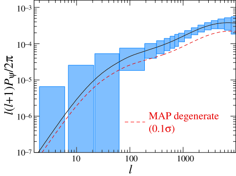
Figure 1.— Weak lensing power spectrum for the fiducial $\Lambda$CDM model and errors for a $\Theta_{\rm deg}=3$ survey. These are compared with a model that is degenerate with respect to CMB measurements from MAP. With the fixed lensing source distribution assumed here for illustration purposes, the $0.1\sigma$ MAP separation increases to many $\sigma$ in the lensing survey.

3. Parameterized Model

Projections for how well weak lensing can measure cosmological parameters depend crucially on the extent of the parameter space considered as well as the location in this space (or “fiducial model”) around which we quote our errors. Previous works have focused on models with essentially two parameters, the matter density $\Omega_{m}$ and the amplitude of mass fluctuations on the 8 $h^{-1}$ Mpc scale today $\sigma_{8}$ (e.g. Bernardeau et al 1997, Jain & Seljak 1997; Jain, Seljak & White 1998). Since all cosmological parameters that affect the amplitude of power across a wide range of physical ($H_{0}\lesssim k\lesssim 10h$Mpc^-1) and temporal scales ($z\lesssim 1$) are accessible to weak lensing, it seems prudent to consider a wider parameter space and then impose any external constraints as prior information.

We consider the adiabatic cold dark matter model space and include 11 free parameters. Weak lensing is only sensitive to 8 of the parameters: the matter density $\Omega_{m}h^{2}$, the baryon density $\Omega_{b}h^{2}$, the mass of the neutrinos $m_{\nu}$, the cosmological constant $\Omega_{\Lambda}$, the curvature $\Omega_{K}=1-\Omega_{m}-\Omega_{\Lambda}$, the scalar tilt $n_{S}$, the value of $P_{\Phi}(3000$ Mpc^-1) initially $A$, and the characteristic redshift of the sources $z_{s}$. The other 3 parameters are necessary when considering prior information provided by the CMB and the galaxy power spectrum because of their covariance with the 8 lensing parameters. These are the optical depth to reionization $\tau$, the primordial helium abundance $Y_{p}$, and the scalar-tensor ratio $T/S$.

For our source redshift distribution we assume a common redshift given by $z_{s}$ since the errors on cosmological parameters are insensitive to the shape of the distribution as long as it is considered known. We return to this point in §6. Our fiducial model is the same $\Lambda$CDM model as chosen in Eisenstein et al. (1998): $\Omega_{m}=0.35$, $h=0.65$, $\Omega_{b}=0.05$, $\Omega_{\Lambda}=0.65$, $m_{\nu}=0.7$ eV, $\tau=0.05$, $n_{S}=1$, $T/S$=0, and $A$ given by the COBE normalization.

4. Cosmological Parameter Estimation

In Tab. 1, we present the Fisher estimates of errors on cosmological parameters from weak lensing assuming full sky coverage $f_{\rm sky}=1$. Errors for more realistic sample sizes scale roughly as $f_{\rm sky}^{-1/2}$. Although these errors (per $f_{\rm sky}^{-1/2}$) are comparable in precision to CMB estimates projected for the MAP and Planck satellites from Eisenstein et al. (1998), they fail to achieve their ultimate potential due to parameter degeneracies. We have included in parenthesis the degradation factors due to degeneracies $(F_{ii})^{-1/2}/(F^{-1})_{ii}^{1/2}$. These are on the order of hundreds and represent the fact that lowering $\Omega_{m}h^{2}$ or $n_{S}$ and raising $\Omega_{b}h^{2}$ all reduce the primordial small-scale power in mass fluctuations whereas raising $\Omega_{\Lambda}$, $\Omega_{K}$ or $m_{\nu}$ all slow the growth rate of structure. These mimic changes in the amplitude $A$ and source redshift $z_{s}$ at the well-sampled high $\ell$’s. On the other hand the observables can basically be characterized by 4 parameters, an amplitude, a slope, the non-linear scale ($\ell\sim 1000$) and the turnover scale ($\ell\sim 100$).

TABLE 1

Full-sky weak lensing survey compared with CMB satellites
$\sigma(p_{i})$ WL MAP Planck $\sigma(\Omega_{m}h^{2})$ 0.024 (430) 0.029 0.0027 $\sigma(\Omega_{b}h^{2})$ 0.0092 (310) 0.0029 0.0002 $\sigma(m_{\nu})$ 0.29 (230) 0.77 0.25 $\sigma(\Omega_{\Lambda})$ 0.079 (180) 1.0 0.11 $\sigma(\Omega_{K})$ 0.096 (200) 0.29 0.030 $\sigma(n_{S})$ 0.066 (470) 0.1 0.009 $\sigma(\ln A)$ 0.28 (310) 1.21 0.045 $\sigma(z_{s})$ 0.047 (56) (1) (1) $\sigma(\tau)$ – 0.63 0.004 $\sigma(T/S)$ – 0.45 0.012 $\sigma(Y_{p})$ (0.02) (0.02) 0.01

Since surveys in the near future will be limited to several degrees on the side at best ($f_{\rm sky}\sim 10^{-3}$), the precision lost to parameter degeneracies is crucial. The combinations of the parameters which are best constrained can be determined by examining the eigenvectors of $F^{-1}$. The best constrained combination of parameters involves $(\Omega_{m}h^{2},\Omega_{b}h^{2},\Omega_{\nu}h^{2}=m_{\nu}/94{\rm eV})$; variation in the direction $(-0.24,0.45,1)$ is constrained to have $1\times 10^{-5}$ amplitude for $f_{\rm sky}=1$. Moving in this direction rapidly reduces the small scale power in mass fluctuations and weak lensing is most sensitive to such variations. From analytic treatments of growth rates, we also expect that neutrinos are twice as effective as baryons in reducing small scale power (Hu & Eisenstein 1998).

These considerations imply that external constraints can help weak lensing measurements regain their precision. CMB satellite missions provide the ideal source of such information since the CMB angular power spectrum they measure is sensitive to the same cosmological parameters but in different combinations. In the example above, the CMB is particularly useful since it can provide precise measurements of $\Omega_{b}h^{2}$ and $\Omega_{m}h^{2}$ leaving weak lensing free to constrain the neutrino mass. Furthermore, it is well known that CMB temperature measurements suffer from degeneracies themselves, especially between $\Omega_{\Lambda}$ and $\Omega_{K}$ along the direction that keeps the angular diameter distance to last scattering fixed. Because $\Omega_{\Lambda}$ must be raised to compensate $\Omega_{K}$ in the CMB angular diameter distance, but must be lowered to compensate $\Omega_{K}$ in the growth rate of structure, one expects that weak lensing will be particularly useful in breaking the degeneracy.

Figure 2 quantifies these expectations. The upper panel shows the improvement over projected MAP satellite errors on cosmological parameters (Eisenstein et al. 1998) when adding the weak lensing information with different survey sizes by summing Fisher matrices. By combining these numbers with those of Tab. 1, one can read off the absolute errors on cosmological parameters. As expected, even a rather modest survey size of $\Theta_{\rm deg}=0.3$ is sufficient to improve MAP errors on $\Omega_{\Lambda}$ and $\Omega_{K}$ by a factor of 3 (see also Fig. 1). Ultimately, weak lensing can improve MAP’s measurement of these quantities by over an order of magnitude. Amusingly, it also improves the measurement of $\tau$ by a comparable factor since the angular diameter distance degeneracy in the CMB requires $\tau$-variations to offset the amplitude changes from $\Omega_{\Lambda}$ and $\Omega_{K}$. Once the degeneracy is broken by weak lensing, $\tau$ becomes better measured. With survey sizes of several degrees and beyond, constraints on $m_{\nu}$ improve to reach the ultimate limit of $\sigma(m_{\nu})=0.1$eV.

Weak lensing can improve on cosmological parameter estimation even if the CMB reaches its full potential with precision temperature and polarization measurements from the Planck satellite (see Fig. 2b). In this case, gains will mainly come from survey sizes $\Theta_{\rm deg}\gtrsim 10$. Again there is the potential to improve measurements of $\Omega_{K}$, $\Omega_{\Lambda}$ and $m_{\nu}$ by nearly an order of magnitude, e.g. $\sigma(m_{\nu})=0.04$eV. This number is of particular interest since the atmospheric neutrino anomaly is currently suggesting mass squared separations of $\Delta m_{\nu}^{2}\sim 10^{-3}$. More generally, this result suggests that weak lensing and CMB measurements can be combined to study the clustering properties of the dark matter and construct consistency tests that can confirm or rule out the presence of a cosmological constant as the component which drives acceleration in the expansion rate.

5. Galaxy Sampling and Distribution

How does the sampling of galaxies and their redshift distribution affect parameter estimation? Kaiser (1998) noted that at degree scales the large ratio of sample variance to noise variance in equation (3) implies that one can obtain better constraints on $P_{\psi}$ here by sparse sampling, provided the power at smaller scales is measured to correct for the aliasing of power. One can estimate the gain in cosmological parameter estimation, under the optimistic assumption that aliasing is negligible, by lowering the number density of galaxies $\bar{n}$ in equation (3) and computing the Fisher matrix as usual. Unfortunately, going from a filled $\Theta_{\rm deg}=3$ survey at $\bar{n}=2\times 10^{5}$ deg^-2 to $\Theta_{\rm deg}=10$ at $\bar{n}=2\times 10^{-4}$ deg^-2 not only does not improve the errors, it can actually degrade them. This is because the main source of cosmological information if $\Theta_{\rm deg}<10$ comes from the translinear regime near $\ell=1000$. Correspondingly in Fig. 2 parameter errors start improving rapidly only if $\Theta_{\rm deg}>10$ due to the resolution of the power spectrum bend below $\ell=100$. Aliasing problems may unfortunately preclude such agressive sparse sampling.

External knowledge of the redshift distribution of the sources can aid parameter estimation especially for survey sizes with $\Theta_{\rm deg}<10$ where $z_{s}$ is not well-measured internally. Redshifts on a fair sample of 100 galaxies would be sufficient to pin down the characteristic redshift to $\sigma(z_{s})=0.1$, improving errors on $\Omega_{\Lambda}$ and $\Omega_{K}$ by up to a factor of two for $\Theta_{\rm deg}<10$. Unfortunately spectroscopy on a fair sample of these faint galaxies may be prohibitive. Alternately one can use photometric redshifts to select a subsample of galaxies whose individual redshifts are known to $\sim 10\%$. For example, even separating the $1.3\%$ of galaxies that are at redshift 3 (Steidel et al.  1996) improve errors on $\Omega_{\Lambda}$, $\Omega_{K}$, and $m_{\nu}$ by a factor of 2.

The actual value of the characteristic redshift itself also affects the sensitivity of weak lensing to cosmological parameters but in a counterintuitive manner. As the characteristic redshift of the source galaxies rise, the lensing effect increases due to the increased amount of intervening large scale structure. Though this makes the signal easier to detect, it does not necessarily imply that errors on cosmological parameters will improve. In fact errors on $\Omega_{\Lambda}$ and $\Omega_{K}$ deprove as the redshift of the sources increases! The reason is that $\Omega_{\Lambda}$ and $\Omega_{K}$ only affect low redshift structure. The intervening high redshift structure is insensitive to these parameters but provide a larger signal whose sample variance swamps the effect of $\Omega_{\Lambda}$ and $\Omega_{K}$. By $z_{s}=3$, errors on $\Omega_{\Lambda}$ and $\Omega_{K}$ degrade by a factor of 6 and 2 for $f_{\rm sky}=1$.

Finally, we have assumed that the galaxy redshift distribution is parameterized by a single number, the characteristic redshift. While this is indeed the main effect (Smail et al. 1995; Fort et al. 1995; Luppino & Kaiser 1997), the fact that weak lensing has the statistical power to measure the characteristic redshift to better than $10\%$ for survey sizes $\Theta_{\rm deg}\gtrsim 10$, implies that more detailed aspects of the distribution, e.g. its skewness, can in principle be measured from large surveys. Allowing the data itself to determine the form of the distribution will of course introduce more uncertainty in the cosmological pararameter determinations, but this would be a small price to pay given the statistical power of such large surveys.

6. Discussion

The Fisher matrix analysis introduced here allows one to explore with ease how assumptions about the survey properties, the fiducial model and any prior knowledge from other cosmological measurements affect parameter estimation. Weak lensing surveys are in principle sensitive to all cosmological parameters that affect the shape of the matter power spectrum, the growth rate of fluctuations, and the source redshift distribution. Here we have included the effects of a cosmological constant, spatial curvature, cold dark matter, baryonic dark matter, hot (neutrino) dark matter, power spectrum tilt and amplitude, and the characteristic redshift of sources. We find that even a relatively modest sample size of $0.3$ degrees would suffice to improve our knowledge of cosmological parameters such as the cosmological constant and the curvature over those provided by MAP satellite measurements of the CMB temperature power spectrum. Order of magnitude improvements in many cosmological parameters are available with survey sizes $\gtrsim 3$ degrees.

We have also explored how properties of the sample affect parameter estimation. Sparse sampling can help extend power spectrum determinations to larger angles but do not necessarily help parameter estimation due to the rather featureless nature of the lensing power spectrum between $100<\ell<1000$. The cosmological constant and curvature can be best measured with a moderate redshift ($z_{s}\sim 1$) population of sources since the larger signal at high redshifts is insensitive to these parameters and act like noise for the purpose of determining those parameters. On the other hand, separating out the $\sim 1\%$ of galaxies at $z_{s}\sim 3$ by photometric redshifts and including this information in the analysis can assist determination of these parameters by up to a factor of 2.

The potential of weak lensing for cosmology explored here will only be realized once systematic errors are reduced below the statistical errors considered here. Anisotropies in the point spread function of telescopes can mask the percent-level cosmological signal and pose a daunting challenge for the current generation of weak lensing surveys. Our analysis reinforces the conclusion that the returns for cosmology justify this great expenditure of effort.

Acknowledgements: We thank R. Barkana, R. Blandford, D.J. Eisenstein, D. Hogg, M. Zaldarriaga for useful conversations. W.H. is supported by the Keck Foundation, a Sloan Fellowship, and NSF-9513835; M.T. by NASA through grant NAG5-6034 and Hubble Fellowship HF-01084.01-96A from STScI operated by AURA, Inc. under NASA contract NAS4-26555.

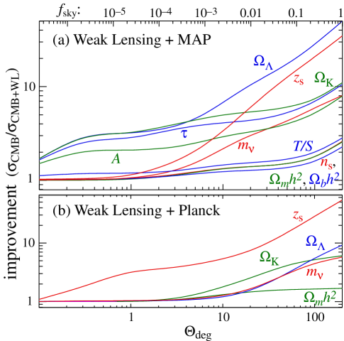
Figure 2.— Improving CMB parameter estimation with weak lensing. We have assumed here and throughout a prior of $\sigma(z_{s})=1$.

References

- (1) Bernardeau, F., Waerbeke, L.V. & Mellier, Y. 1997, A&A 322, 1
- (2) Blandford, R.D., Saust, A.B., Brainerd, T.G., & Villumsen, J.V., MNRAS, 251, 600
- (3) Eisenstein, D.J., Hu, W., & Tegmark, M., ApJ (submitted)
- (4) Fort, B., Mellier, Y. & Dantel-Fort, M. 1997, A&A, 321 353
- (5) Hu, W. & Eisenstein, D.J. 1998, ApJ, 498, 497
- (6) Jain, B. & Seljak, U. 1997, ApJ, 484, 560
- (7) Jain, B., Seljak, U., & White, S.D.M (in preparation)
- (8) Kaiser, N. 1992, ApJ, 388, 272
- (9) Kaiser, N. 1998, ApJ, 498, 26
- (10) Luppino, G. & Kaiser, N. 1997, ApJ, 475, 20
- (11) Miralda-Escude, J. 1991, ApJ, 380, 1
- (12) Peacock, J.A. & Dodds, S.J. 1994, MNRAS, 267, 1020
- (13) Seljak, U. 1998, ApJ, 506, 64
- (14) Smail, I., Ellis, R., & Fitchet, M. 1995, MNRAS, 273, 277
- (15) Smail, I., Hogg, D.W., Yan, L., & Cohen, J.G., ApJL, 449, L105
- (16) Steidel, C.C., Giavalisco, M., Pettini, M., Dickinson, M., & Adelberger, K.L., ApJL, 462, L17